


Introduction
As the field of polar remote Sensing turns increasingly from basic algorithm demonstration to change detection, the value of long-term calibrated and validated Satellite datasets increases. moreover, inter-calibration of datasets derived from different Sensors becomes important as a means of extending the temporal record for detection of change. here we link a 22 year record of ice Surface Skin temperature (1981–2003) derived from the advanced very high resolution radiometer (AVHRR) with a 6 year (2000–06), and growing, Sea-ice temperature record produced from the moderate-resolution imaging Spectroradiometer (MODIS).
The 22 year record of avhrr ice temperature comes from the avhrr 5 km and 1.25 km polar pathfinder DATASET, created and distributed by the us national Snow and ice data center (NSIDC; Reference Maslanik, Fowler, Key, Scambos, Hutchinson and EmeryMaslanik and others, 1997). the dataset Spans the period 1981–2000 at 5 km, and 1993–2003 at 1.25 km (including archived level 1B Swath data at 1.1km nadir resolution), and includes data from the us national oceanic and atmospheric administration’s NOAA-7, 9, 10, 11, 12, 14, 15 and 16 polar-orbiting Satellite platforms. the MODIS-derived Sea-ice Surface temperature product (sea ice extent 5 min Swath 1 km product; Reference Hall, Key, Casey, Riggs and CavalieriHall and others, 2004) is a 1 km level 2 Swath product of the earth observing System data product System. it is a cloud-masked dataset, available for both terra and aqua modis Sensors for the period february 2000 (terra) or july 2002 (aqua) to the present (data products MOD29 and MYD29).
Arise Cruise
The antarctic remote ice Sensing experiment (arise) of September–october 2003 had as its mission the observation of antarctic Sea-ice characteristics, and the validation of a number of remote-sensing-derived measurements over Sea ice in antarctic Sea-ice conditions (Reference MassomMassom and others, 2006). this mission of the Aurora Australis used Ship-board Sensors, direct measurements and helicopter-mounted and -towed platforms to Survey an extensive area of east antarctic Sea ice during Spring conditions (fig. 1). in addition to these ice Surface temperature validation measurements, extensive calibration–validation Studies were conducted to verify passive microwave-derived extent and concentration, visible/near-infrared albedo, thickness and Snow-cover algorithms for Sea-ice Study. algal System Studies at the ice edge and throughout the Southern ocean were also conducted.
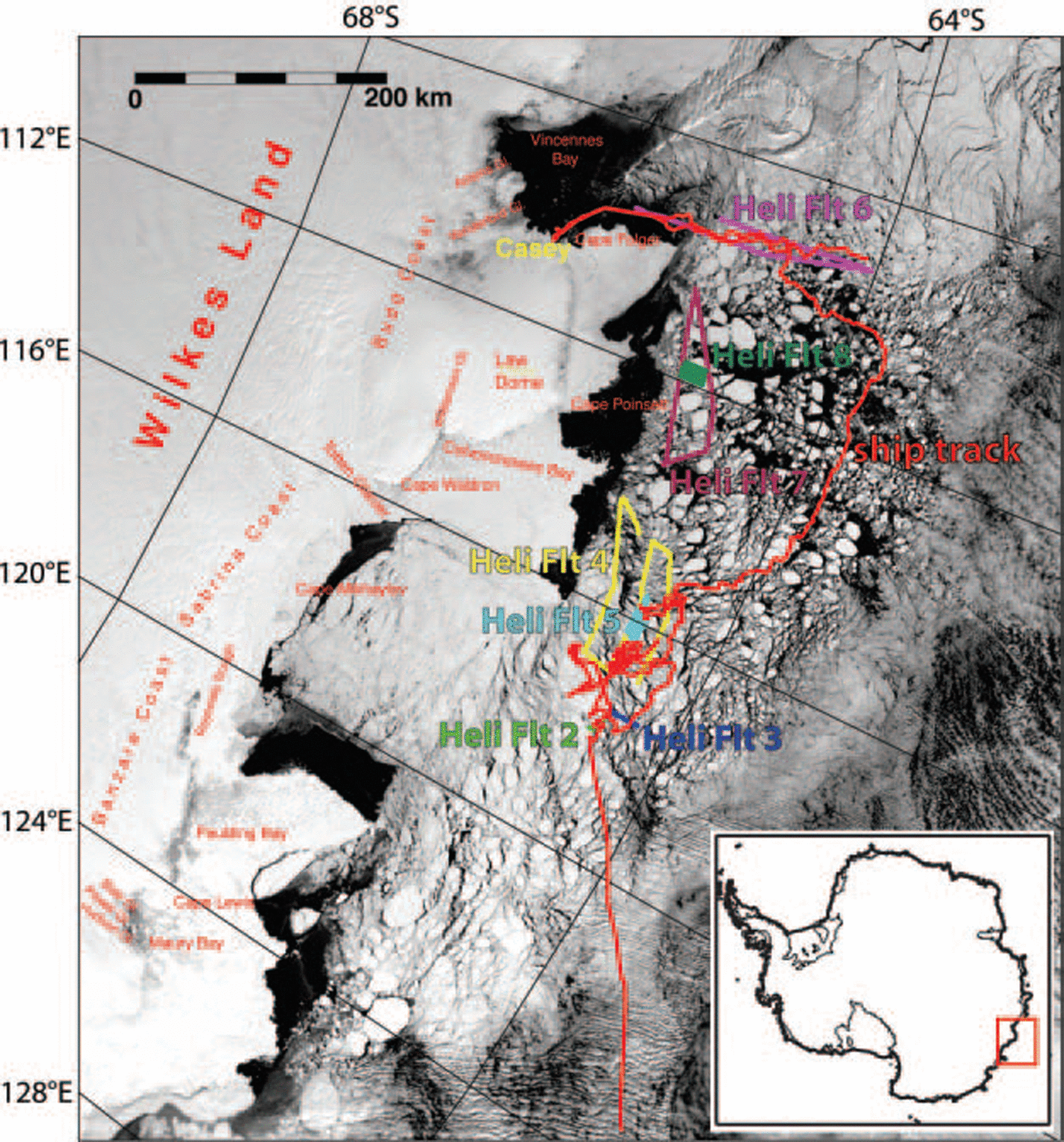
Fig. 1. Image map derived from a Terra MODIS image from 20 October 2003 (0135 UT acquisition time), Showing the course of the ARISE cruise (red line) between 25 September and 21 October 2003, and tracks of helicopter flights with validation data (‘Heli Flt’ 2–8, various colors). ‘Heli Flt 2’ (green) was acquired on 3 October; ‘Heli Flt 3’ (blue) on 3 October; ‘Heli Flt 4’ (yellow) on 8 October; ‘Heli Flt 5’ (cyan) on 8 October; ‘Heli Flt 6’ (magenta) on 19 October; ‘Heli Flt 7’ (maroon) on 20 October; and ‘Heli Flt 8’ (dark green) on 20 October. The image Shows Sea-ice conditions (approximately) for only the last three helicopter flights.
Satellite Sensor Ice Surface Temperature Algorithms
Ice Surface Skin temperature is derived by measuring thermal-band emission (8–14 μm) from the Snow Surface (Reference Key and HaefligerKey and haefliger, 1992; Reference ComisoComiso, 1994; Reference Lindsay and RothrockLindsay and rothrock, 1994). high emissivity of Snow and a low atmospheric absorption in this range make this measurement feasible and relatively easy to calibrate. both algorithms used here apply the Split-window technique, based on
Where T s is the measured Skin emission temperature, a, b, c and d are constants derived from a regression of calibration data, σ is Sensor Scan angle through the atmosphere, and T 11 and T 12 are thermal channel brightness temperature measurements in the 11 and 12 μm range. for avhrr, channels 4 (10.3–11.3 μm) and 5 (11.5–12.5 μm) are used; for modis, bands 31 (10.78–11.28 μm) and 32 (11.77–12.27 μm). calibration data for the regression come from polar-region radiosondes coupled with a radiative transfer model (LOW-TRAN; See Reference Hall, Key, Casey, Riggs and CavalieriHall and others, 2004). for the avhrr polar pathfinder dataset, the Split-window approach is only possible with the AVHRR-3 Sensor; the NOAA-10 Sensor permits only a Simpler algorithm using just channel 4 (AVHRR-2 Sensor; See Reference Hastings and EmeryHastings and emery, 1992; Reference Maslanik, Fowler, Key, Scambos, Hutchinson and EmeryMaslanik and others, 1997). avhrr Sensor Series regression parameters are provided by Reference Key, Collins, Fowler and StoneKey and others (1997) and j. key (personal communication, 2003). modis regression parameters are given in Reference Riggs, Hall and AckermanRiggs and others (1999; any updates to avhrr or modis ice Surface temperature parameters are available by request to NSIDC).
In Situ Measurement Methods and Comparison With Satellite Data
Validation of the two Satellite-based temperature products was accomplished by comparing Satellite-derived Skin temperatures in the regions Surrounding the Ship with in Situ and airborne thermal radiometer measurements of the ice Surface under clear-sky conditions. two radiometers were used: a rail-mounted Sensor imaging an area adjacent to the Ship; and a Similar device mounted to a nadir viewport on a helicopter (fig. 2).
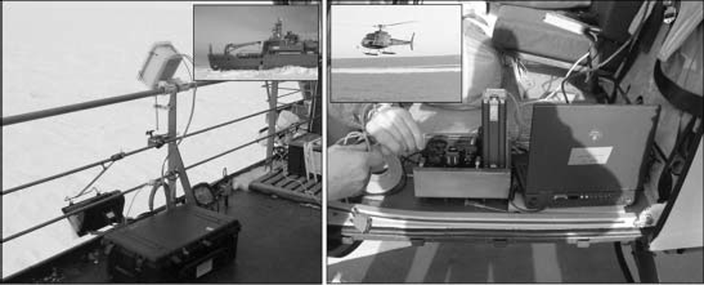
Fig. 2. Photographic collage illustrating in Situ KT-19 radiometer measurement helicopter (right) and Ship’s-rail (left) configurations.
Rail-mounted System
The thermal radiometer used for the rail was a heitronics kt-19.82, measuring the Spectral range 8–14 μm. the device was mounted to the port Side rail and pointed at the ice (or water) Surface adjacent to the Ship at a Surface viewing angle of 60–30˚ below the horizon, with 30˚ as the nominal value. Several tests of Sensitivity to viewing angle (over the range 60–15˚) Showed brightness temperature variations of just Several tenths of a kelvin, with usually lower temperatures at high incidence angles, but variable. the 30˚ viewing angle was Selected to place the viewing area well to one Side of the Ship, minimizing the effects of Ship Splash and fresh fractures while underway. Spot measurement area is roughly 0.5 m across, given the rail height of 15 m, the field of view of the instrument, and the 30˚ viewing angle. the radiometer was Set in a foam-insulated box, and a Self-regulating resistance heating System was installed to keep the instrument temperature at 280±3 k. a data rate of 1 S was used. the device recorded brightness temperatures in kelvins (i.e. assuming an emissivity of 1.0 for all Surfaces). Sensitivity of the device (rms of a constant-temperature Surface at 1 S integration) was reported by the manufacturer as being 0.1 k. the accuracy of the device was checked before and after most runs by viewing a fresh ice-water bath. with emissivity Set to 1, under clear Skies, this test consistently reported temperatures of 272.2–272.6 k (see below for later correction for emissivity). data were acquired for continuous multi-hour periods, Spanning Several overflights of the Noaa-12, Noaa-15 and Noaa-16 Satellites, and the terra and aqua Satellites, during both day and night. approximately 20 observing Sessions were conducted over the period 25 September–21 october 2003 (fig. 3).

Fig. 3. Validation of Avhrr Polar Pathfinder ice Surface temperature (a) and Modis Sea-ice Surface temperature (b) using Ship-rail-mounted KT-19.82 data. Ranges of image-grid pixel values at each calibration Site Shown by triangles above and below the mean value. Error of KT-19.82 measurement Shown by width of box Symbol (±0.3 K). Best-fit line, with equation, Shown for both Sensors (thick dashed line); 1 : 1 line (solid), with lines at 2.5 K above and below the 1 : 1 reference (thin dotted lines) are also Shown.
After acquisition, data were averaged to 1 min intervals and compared with Several additional parameters acquired during the cruise: global positioning System (GPS) position, GPS-derived Speed, Ship’s air temperature (21m above the Sea Surface), Solar incoming radiation (a further indicator of cloudiness), wind direction and Speed, and data from another radiometer aboard, maeri (marine–atmosphere emitted radiance interferometer; See Reference Kearns, Hanafin, Evans, Minnett and BrownKearns, 2000; Reference Minnett, Knuteson, Best, Osborne, Hanafin and BrownMinnett and others, 2001). in addition to minute-averaged mean kt-19 Sensed temperature, the minimum, maximum and Standard deviation for the 60 S interval was recorded. maeri data reported a Skin temperature of the Surface given an emissivity, ε, of 0.9627 (value appropriate for Sea water; Reference Kearns, Hanafin, Evans, Minnett and BrownKearns and others, 2000), averaged over 12 min.
Helicopter-mounted System
A heitronics kt-19.85, Sensing emissions over a 9–11 μm range, was mounted to a nadir-viewing rack on a helicopter and flown on three days (29 September, 8 and 20 october 2003) for Several hours in the vicinity of the Ship (figs 1 and 2b; See also Reference MassomMassom and others, 2006, fig. 6). these data were acquired every 2 S. the radiometric resolution for the instrument at this rate is given by the manufacturer as ±0.1 k. the altitude of the helicopter was ∽1500m (5000 ft). at this height, the Spot viewing area is ∽65m diameter. the helicopter unit was not temperature-controlled, and internal temperatures varied from 275 to 295 k.

Fig. 4. Helicopter validation flight of 8 October. (a) Regional Sea-ice extent and clouds Shown in Modis Channel 1 image (250m pixel Size) acquired during the flight (Aqua, 0820 UT). (b) Close-up of helicopter ground track. (c) Modis-derived Sea-ice Surface temperature and cloud mask image. (d) Noaa-16 Avhrr-derived ice Surface temperature (acquisition time 0832 UT). A Noaa-12 image was also acquired during the flight (not Shown; acquisition time 0847 UT). (e) Along-track KT-19.85 Skin temperature variations with time, as well as Aqua Modis, Avhrr Noaa-16 and Noaa-12 values at the track locations. Vertical colored bars Show time range of ±400 S, used in Figure 5 for validation. Note drift in temperature over ice floes in the black KT-19 track due to diurnal temperature change; line fit Shown (black) is used in Figure 6to evaluate diurnal cooling in the Modis-to-Avhrr comparison.
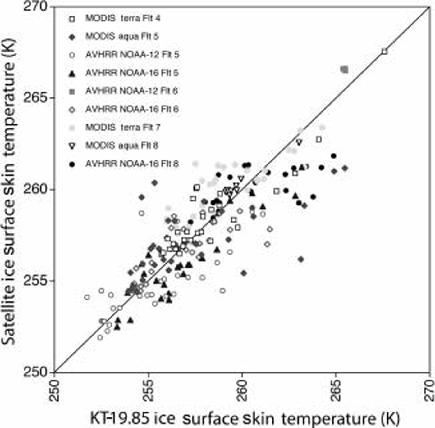
Fig. 5. Helicopter-mounted KT-19.85 ice Surface Skin temperature vs Satellite-derived ice Surface temperatures. Each observation Set represents 800 S of KT-19 measurements bracketing the time of Satellite data acquisition. KT-19 Spot measurements are averaged for each 1.25 km of track distance.
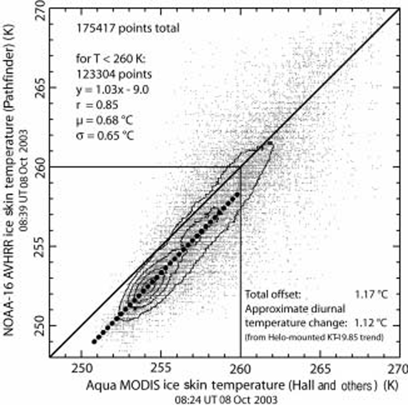
Fig. 6. Cross-plot of clear-sky pixels (using MODIS product cloud mask) from area Shown in Figure 4a for both MODIS-derived and AVHRR-derived Sea-ice Skin temperature during helicopter flight. Contour lines indicate increasing data density near best-fit line. Fit line was determined using only data where T < 260 K (see text).
Emissivity correction
Emissivity corrections (e.g. correction from brightness temperatures to Skin temperatures) were applied to the rail-mounted radiometry data by the following equation:
Where T skin is the corrected ice Surface Skin temperature, T BTice is the brighness temperature of ice, and T BTsky is the mean all-sky brightness temperature. this follows a Similar approach taken for the maeri Sensor in the measurement of ocean temperature (Reference Kearns, Hanafin, Evans, Minnett and BrownKearns and others, 2000). in the Sensitivity range of the rail-mounted kt-19.82 (8–14 μm), the mean Spectral emissivity, ε, of Snow/ice at a 30˚ Surface incidence viewing angle is 0.985 (Reference Dozier and WarrenDozier and warren, 1982); it ranges from ∽0.981 (15˚ incidence) to 0.997 as the viewing angle approaches vertical. with the 30˚ viewing angle for the rail-mounted System, it is necessary to correct for the 0.015 reflectivity factor, using an estimate of the clear-sky brightness temperature (direct measurements of clear Sky by the kt-19 always fell below its Sensitivity limit of ∽220 k). we used 200 k for this value. for the helicopter-mounted kt-19.85, the Sensitivity range (9–11 μm) has a mean ice emissivity that is higher at all incidence angles, and is 0.998 under nadir-viewing conditions (Reference Dozier and WarrenDozier and warren, 1982). given this, and the uncertainty of the full-sky brightness temperature above the viewing point of the helicopter-mounted Sensor, an ε value of 1.0 was used and no Sky correction was applied.
Error of the KT-19 measurements
Noise levels for the kt-19.82 and kt-19.85 are noted above. in our in Situ measurements, Stationary observing periods for the kt-19.82 on the rail of the Ship often Showed long periods where variations were less than this, 0.05–0.07˚c. with 1 min averaging, Standard deviation during Stationary viewing of uniform ice was typically 0.02–0.03˚c. given this, the main error Source is presumed to be the Sky correction. our estimated all-sky brightness temperature of 200 k could vary by up to 20˚c, depending on humidity and/or the presence of Scattered or thin clouds. with a 20˚c variation, the corrected kt-19 value Shifts by 0.35 k, and we take this value as our likely error for the Ship’s-rail (kt-19.82) measurements. for the helicopter-mounted radiometer, the lack of a Sky correction results in a ∽0.4˚c error, i.e. Skin temperatures too cold by this amount assuming Sky brightness temperatures of ∽200–220 k.
Satellite images
Satellite data images from the avhrr Sensor on the Noaa-12, Noaa-15 and Noaa-16 Satellites were down-linked as they flew overhead by the terrascan System on Aurora Australis. the Satellite data were processed using polar pathfinder algorithms identical to those used in the main Nsidc-based datasets for both albedo and ice Surface temperature. these data were gridded to a 1.25 km grid in the polar pathfinder projection (lambert equal area polar azimuthal). no cloud masking was applied; clear or cloudy Sky conditions were determined by meteorological notes from aboard the Ship, and examination of the albedo and thermal images. for the modis data, we requested MOD29 and MYD29 Swath products for the Same days that were Shown to have large clear-sky areas in avhrr, and for which we had kt-19 measurements. these Swath products were then gridded to the Same polar pathfinder grid using the modis Swath to grid toolbox (ms2GT) Software available from Nsidc.
Selection of validation points for the rail-mounted System
There were Several factors considered in the Selection of Satellite-derived pixel values of Skin temperature and mean kt-19 data for comparison. these are a result of the Sub-gridcell Spatial variability of the Surface (sea ice and leads), the variation of temperature over time, and the movement of the Ship through thick or thin ice. the Ship, which typically followed open-water or light-nilas covered leads, was often on a boundary in temperature represented by a mixed-surface pixel in the gridded images. for this reason, nearby pixels, covering areas that were interpreted to be homogeneous at the 1.25 km Scale, were used for comparison with the rail-mounted kt-19 temperatures. moreover, the geo-registration of the avhrr data using only the Satellite ephemeris (conducted on board) results in geolocation errors of 3–7 km. these issues were avoided by Selecting four to eight nearby gridcell pixels in regions of uniform brightness temperature (e.g. from large floes or uniform nilas/thin-ice areas) within a radius of ∽15km of the Ship. the kt-19 measurements are Selected from times close to (±30 min) the acquisition times that represented periods when the port Side of the Ship Saw a uniform Surface type for Several minutes. for example, if the measurement was over thick Snow-covered ice floes, Several nearby cold-floe areas from the images were compared with the coldest, lowest-variability minute-averaged measurements from the kt-19 record. for leads and polynyas (usually covered with thin grey to grey-white nilas) a Similar approach was used, taking uniform but warmer temperatures from both the image data and kt-19 record. open-water contamination was eliminated by Selecting 60 mean points for which the maximum 1 S temperature was <269 k. a Similar approach was used for the Modis–ship’s-rail comparison, but here geo-referencing errors are within 50m (Reference WolfeWolfe and others, 2002), and resolution is Somewhat better (1.0 km), So comparison points could be kept within 5 km of the Ship position.
Validation using the helicopter-mounted radiometer
Helicopter flights with remote-sensing data at the time of Satellite overflights occurred on 8, 19 and 20 october 2003. helicopter flights were typically 30 min to 3 hours in duration. we identified Seven avhrr and Six modis Scenes with acquisition times during the aerial radiometer collection.
The high resolution and extensive track length of the airborne radiometer requires that the Satellite data be precisely geolocated, and that cloud areas are masked. to geolocate the avhrr data, we Shifted the image grids to a best-fit match with the closest modis image. usually these Scenes were within 1 hour of each other, minimizing the effect of Sea-ice drift in the interval. we also used the modis cloud mask to eliminate cloud-impacted pixels and Spots from the avhrr and kt-19.85 profile data.
figure 4 provides an example of the airborne radiometer data and near-simultaneous Satellite data. as Shown in figure 4e, the airborne radiometer acquires a much higher-resolution profile than the Satellites are capable of resolving. at the typical Speed of flight of the helicopter (∽40ms–1), radiometer data are acquired every ∽80m with ∽65m diameter averaging. this easily resolves narrow leads (skin temperature of 267–270 k) and thermal gradients across floes. furthermore, during the period of the flight, the mean Surface temperature varies. in the figure 4e example, the mean temperature of the floe Surfaces cools about 7 k during the 95 min flight. to determine the rate of cooling for direct intercomparison of image-derived temperatures, discussed below, we eliminated points with T > 260 k and fit a trend line. warmer temperatures were eliminated because these Surfaces are influenced more by the underlying ocean water, and are thus buffered (and So do not Show the evening cooling trend).
To compare the narrow, hours-long Spot tracks of the helicopter-mounted radiometer with the coarser-resolution, near-instantaneous Satellite radiometers, we both Smoothed the aerial-based data and narrowed the time window of comparison. profile data were Smoothed by averaging 1.25 km Segments of the tracks. we used an 800 S time window centered on the time of Satellite image acquisition to reduce the effects of diurnal Surface temperature change. these constraints reduced the total number of valid Scenes to five avhrr and four modis.
Results and Discussion
Ship’s-rail-mounted validation results
For Avhrr data, 41 overpass periods (‘sites’) were acquired where Skies were clear (less than two-tenths Sky cover) and kt-19 data were acquired (fig. 3a). Skin Surface temperatures at the Sites ranged from 243 to 269.5 k. Sites over a broad variety of ice types were used, including thick first-year floes, light nilas and thin Smooth floes. wetted ice or very young thin-ice types were avoided because of the uncertainty of the emissivity and emissivity correction. for modis data, 17 Sites were identified (fig. 3b). modis Sites were fewer because timing of kt-19 acquisitions was Set to favor avhrr overpasses, and three avhrr Sensor platforms were available vs two modis platforms.
The relationship between kt-19.82 measurements and the temperature at nearby pixels is highly linear for both Sensors. AVHRR data Show a high correlation (r = 0.97) and a nearly 1 : 1 Slope with the Ship-board measurements. no differences were Seen among the three AVHRR Sensors used, validating the Separate calibrations of these platforms (the NOAA-12, -15 and -16 avhrr Sensors). for modis, the correlation was Similarly high (r = 0.98), but the data Showed a distinct Slope and offset. we attribute this to the lower number of Sites, and the narrower range of Site temperatures, and not to a real effect of the Sensor or algorithm. data for both avhrr and modis fall close to the 1 : 1 line (±1.0 k for modis; ±1.4 k for avhrr, 1σ).
Helicopter-mounted validation results
figure 5 Shows ice Surface temperature data from the nine Satellite images and the corresponding kt-19.85 aerial measurements. individual Scene–radiometer combinations Show Significant Scatter, but the trend for all data is highly linear and almost all lies within 2.5 k of the 1 : 1 relationship (±1.7 k, 1σ for 236 Sites total). we were unable to justify a quantitative linear fit for each of the observation pairs, or for any of the Sensors individually. as with the Ship’s-rail data, Scatter in the data is likely due to mixed-pixel and co-registration issues, despite our attempts to reduce these effects.
Direct comparison of Modis and Avhrr ice Skin temperatures
figure 6 is a cross-plot of temperature data from the 8 october aqua modis data collection and the NOAA-16 avhrr data from the Same date (see also fig. 4). the acquisition time for the center of the Study region differed by 15 min for the two Sensors, 0824 ut for modis and 0839 for avhrr. during this period, Significant cooling occurred over the region as local Sunset approached. as Shown in figure 4, this trend of cooling was approximately 4.5˚ch–1. however, over thin ice and open water no cooling is observed, because of a buffering effect of relatively warm ocean water.
As implied by that effect, the figure 6 cross-plot Shows a colder trend for the later avhrr image, but also a Steeper Slope towards less-cooled thin-ice and open-water temperatures that are thermally buffered by the ocean. to determine the trend in figure 6, we eliminated those gridcells with temperatures greater than 260 k. this resulted in a highly linear (r = 0.85), near-unity (slope = 1.03) relationship between the two products, with a very low mean Scatter and Standard deviation from the trend (0.68˚c and 0.65˚c respectively). we consider this to be the best evidence of excellent precision and accuracy in both products. we attribute the observed Slope in the trend for the two Sensors to be a residual effect of the ocean warming of thinner ice.
Air-temperature inversions and air-temperature–skin-temperature differences
Air temperatures were recorded during all Ship’s-rail observations by the arise cruise meteorological Staff. the temperature Sensor was located 21 m above the waterline. during the course of the validation experiments, we noted large differences between the kt-19.82 ice Surface Skin temperature measurements and this air temperature whenever clear-sky and low-wind conditions prevailed (fig. 7). temperature differences of 2–15˚c were observed, and these formed and decayed rapidly (tens of minutes) as clouds moved into and out of the zenith area. we attribute this to Strong atmospheric thermal inversions forming rapidly under clear-sky conditions, and breaking down when clouds covered most of the Sky.
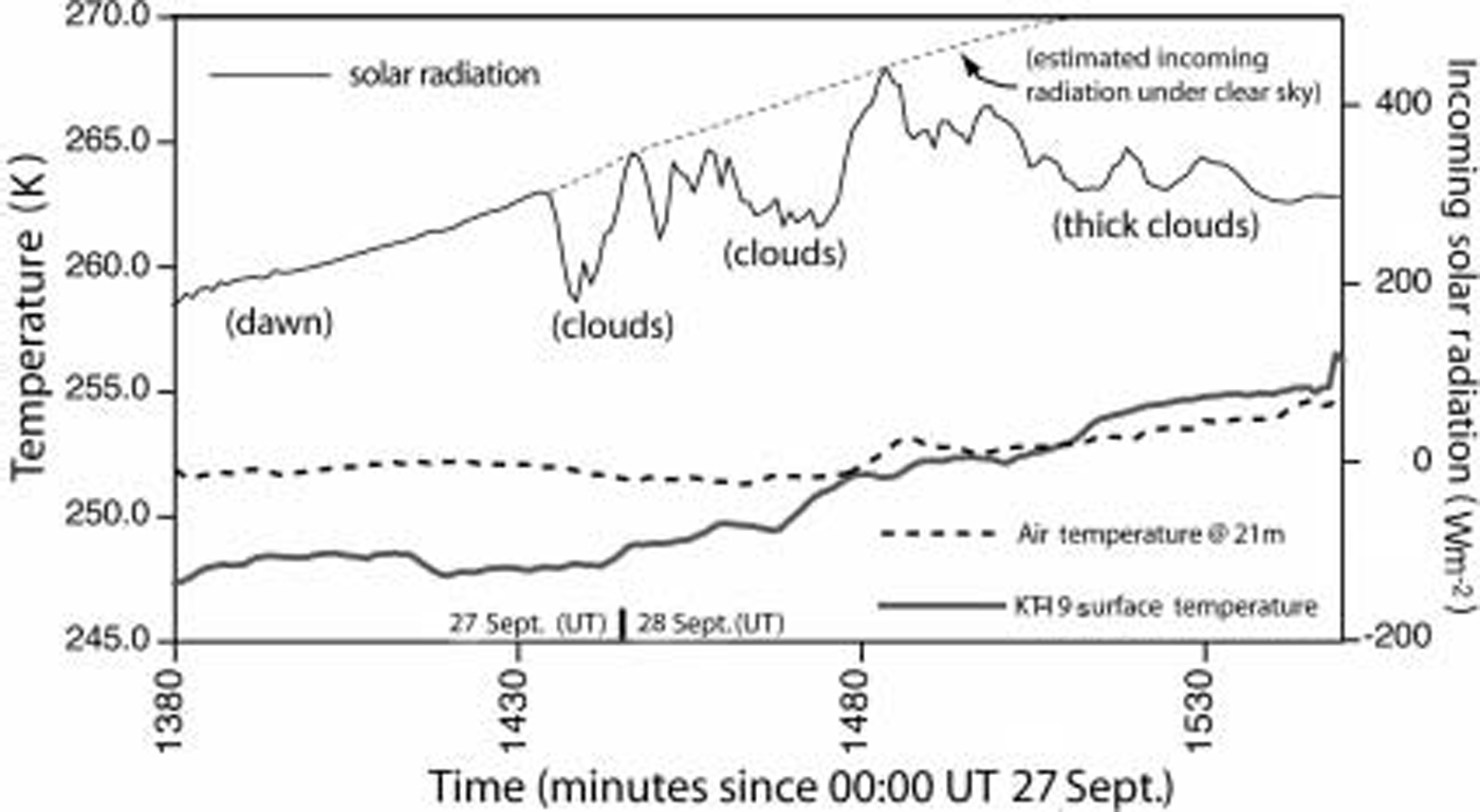
Fig. 7. Air temperatures and Sea-ice Surface Skin temperatures during transition from clear to cloudy periods. Strong Surface inversion forms under clear-sky conditions, and breaks down within 15–30 min of cloud cover.
Thermal inversions are common polar occurrences; however, these inversions had gradients intense enough (0.25 km–1) to Significantly affect a comparison of meteorological Station or automated weather Station (AWS) 2 m air temperatures and Satellite measurements of ice Surface Skin temperature. Reference Hall, Key, Casey, Riggs and CavalieriHall and others (2004) used 2 m air temperatures from South pole and various arctic Sites in their calibration/validation of the ice Surface temperature algorithm, and they observed a consistent offset (∽0.9 k) with the Satellite value being lower. moreover, Reference ComisoComiso (2000) and many others attempt to use air temperatures to calibrate Surface Skin temperature measurements, generally using clear-sky data. this Study Shows that Such comparisons may Suffer from this near-surface inversion gradient.
Conclusions
Our results Show that both the AVHRR polar pathfinder and MODIS-based ice Surface temperature algorithms have highly linear, near-1 : 1 relationships with in Situ radiometric measurements. however, in both our validation experiments, mixed-pixel and co-registration effects (particularly difficult issues with Sea-ice targets) probably reduce the perceived accuracy of the algorithms below their true levels. nevertheless, our data Show that the Satellite-derived products are valid for all ice-type targets over the 245–270 k range to within at least ±1.5˚c, and probably ±0.7˚c based on a direct comparison of the two Satellite Sensors with Simultaneous in Situ radiometer measurements (fig. 6). this refines the earlier air-temperature-based validations reported by Reference Hall, Key, Casey, Riggs and CavalieriHall and others (2004), in their initial discussion of the MODIS-based ice Surface temperature algorithm. we further find that near-surface temperature inversions can be Strong enough under cold, clear conditions to affect air-temperature–satellite-based ice Skin temperature comparisons.
Acknowledgements
We acknowledge with gratitude the Support of the captain and crew of the Aurora Australis. images and other Satellite data required during the cruise were provided by j. bohlander and j. Smith of NSIDC. meteorological data were provided by d. allen, S. visentin and j. golding; comparison data from the maeri ocean/ice radiometric Sensing equipment were provided by e. key and p. minnett. R.M. was Supported by the australian government’s cooperative research centres programme through the antarctic climate and ecosystems cooperative research centre (ace crc) and asac project 2298. T.S. and T.H. were Supported by nasa grant NAG5-11308 and the nasa Snow and ice distributed active archive at NSIDC.


