


1. Introduction
Understanding the pathways for infection transmission in hospitals and other buildings is critical for managing epidemics such as the present Covid-19 pandemic. Although there is debate about the dominant pathways for respiratory virus transmission (Beggs Reference Beggs2003; Tellier Reference Tellier2006), there is evidence that aerosols are produced by breathing, talking, coughing and sneezing (Duguid Reference Duguid1947; Gupta, Lin & Chen Reference Gupta, Lin and Chen2009; Bourouiba, Dehandschoewercker & Bush Reference Bourouiba, Dehandschoewercker and Bush2015) and that these can carry viable virus (Milton et al. Reference Milton, Fabian, Cowling, Grantham and McDevitt2013). Although these droplets may partially evaporate, typically 5 %–10 % of the droplet may be non-volatile (Tang Reference Tang2009; Liu et al. Reference Liu, Wei, Li and Ooi2017), and these form a droplet nucleus with radius 0.36–0.45 of the original droplet size that can contain a pathogenic microorganism (Wells Reference Wells1934; Papineni & Rosenthal Reference Papineni and Rosenthal1997). The volatile component of droplets initially smaller than 10  $\mathrm {\mu }$m typically evaporate in 1–10 s (cf. Liu et al. Reference Liu, Wei, Li and Ooi2017), and so the associated, non-volatile nucleus may remain suspended for over 20 minutes, given the time for a 4 $\mathrm {\mu }$m droplet to fall 2 m is over 1000 s (Wan & Chao Reference Wan and Chao2007; Liu et al. Reference Liu, Wei, Li and Ooi2017).
The dispersion of such droplets is controlled by the ventilation flows, convection resulting from temperature differences in the space, and mixing and dispersion produced by the movement of people through the space (Hoffman, Bennett & Scott Reference Hoffman, Bennett and Scott1999). Typical ventilation flow speeds may be of order  $0.1\text {--}1.0$ cm s $^{-1}$ (Etheridge Reference Etheridge2011), while convective flows produced by heating systems or thermal mass may have a scale as large as 1–10 cm s $^{-1}$ (Linden, Lane-Serff & Smeed Reference Linden, Lane-Serff and Smeed1990; Gladstone & Woods Reference Gladstone and Woods2001). In contrast, people moving through a space have speed of order $1.5\pm 0.5$ m s $^{-1}$, and so drive a wake flow which may be an order of magnitude larger than the ventilation flows, with typical length scales of 0.5–1.0 m, given the typical dimensions of people (Wu & Gao Reference Wu and Gao2014). Wake-driven mixing has the potential to be very significant during the time scale over which the ventilation flow replenishes the air, and the continued mixing of new and old air may cause a concomitant increase in the age of airborne aerosols while reducing their concentration (cf. Wang & Chow Reference Wang and Chow2011).
There have been many studies exploring the mixing of air in rooms subject to ventilation flows, and in many cases these studies suggest that the air is mixed with an effective dispersion coefficient in the space. Cheng et al. (Reference Cheng, Acevedo-Bolton, Jiang, Klepeis, Ott, Fringer and Hildemann2011) carried out an experimental study involving two naturally ventilated rooms, with ventilation rates ranging between 0.2 and 5.4 air changes per hour, and estimated that a tracer gas released into the rooms was subjected to turbulent diffusion with an effective diffusion coefficient of order  $D_v\approx 10^{-3}{-}10^{-2}$ m $^2$ s $^{-1}$. Foat et al. (Reference Foat, Drodge, Nally and Parker2020) describes the outcome of similar experiments in a meeting room with mechanical ventilation, with inlet and outlet vents located at the level of the ceiling. A tracer gas was released in the room and its decay was monitored using sensors. Based on the transient concentration of the tracer, the effective diffusion coefficient was again estimated to be of order $D_v\approx 10^{-2}$ m $^2$ s $^{-1}$. Comparable results were obtained by Nomura et al. (Reference Nomura, Hopke, Fitzgerald and Mesbah1997), Nicas (Reference Nicas2009) and Shao et al. (Reference Shao, Ramachandran, Arnold and Ramachandran2017).
In this paper we explore quantitatively the mixing which may arise from the movement of people along a corridor through a series of controlled and simplified analogue experiments. We use a small scale channel filled with water and move a cylinder back and forth along the channel to represent a person walking. We inject a pulse of dye in the centre of the channel, and use a light attenuation method to track the gradual dilution of the dye along the channel. After many passages of the cylinder, we find that the dye becomes dispersed, and eventually well mixed throughout the channel. We analyse the quantitative data through a series of systematic experiments to develop a model for the effective dispersion coefficient of the moving cylinder, and show that the model is consistent with the early- and late-time mixing of the dye. We compare our results with earlier estimates of the effective diffusion coefficient in ventilated rooms, and apply them to provide some simple predictions for the dispersal distance of airborne aerosols in a corridor, prior to their ventilation.
2. Experimental apparatus
We used two different tanks during these experiments to explore the sensitivity to different parameters. First we conducted a series of experiments using a tank 20 cm deep, 104 cm long and 10 cm wide, containing water to a depth  $H=18$ cm (see figure 1). A series of four cylinders of diameter 1.5, 2.5, 4 and 5 cm were, in turn, placed in the tank and moved back and forth along the whole length of the tank, up to within 5.6 cm of the end walls, using a motorised traverse system, with a speed $u$ ranging between 9.0 and 26.2 cm s $^{-1}$. A fluorescent light panel was placed behind the tank and provided uniform illumination, and the motion of a known pulse of dye released in the centre of the tank was recorded using a JAI SP-5000 high-speed digital camera located 5 m from the tank (see figure 1). The camera captured 60 to 200 frames per second in different experiments, with a resolution $1650 \times 300$ pixels. In a second series of experiments, to investigate the effects of a different channel length and width, we used a different tank of dimensions $20\ \text {cm} \times 265\ \text {cm} \times 15\ \text {cm}$, but with the same set of cylinders.

Figure 1. Schematic representation of the experimental apparatus.
Table 1 summarises the conditions of all experiments carried out. At the start of each experiment, a known mass of neutrally buoyant dye was added to the centre of the tank. The initial dye concentration in the pulse was of order  $c_0\approx 0.10\pm 0.02$ g L $^{-1}$, and the ratio between the length of the region of dyed fluid at the beginning of an experiment and the length of the tank was $0.10\pm 0.05$. Hence, towards the end of each experiment the well-mixed uniform dye concentration in the tank was of order $c_\infty \approx 0.01$ g L $^{-1}$. In order to obtain quantitative information, the line-of-sight width-averaged light intensity was measured at each point in the tank throughout each experiment. This width-averaged light intensity was calibrated using a series of test experiments in which dye solutions of different concentration, ranging between $c_0$ and $c_\infty$, were added to the tank to generate a calibration curve. We note that during an experiment, a very small portion of the fluid in the tank (of order 5 % or less) was obstructed by the opaque oscillating cylinder. The concentration of dye in this region was estimated using linear interpolation of the surrounding concentration field. Although this introduced some error, the accuracy of the light attenuation technique and of the described linear interpolation was tested in each experiment by estimating the total mass of dye in the tank at each time using the light attenuation calibration. We found that during each experiment this was a constant with an error of less than $2\,\%$. In this way, the depth-averaged concentration of dye, $c(x,y,t)$ was measured at each time, $t$, and each point, $(x,y)$, on a vertical plane parallel to the side wall of the tank, where $0<x<L$ and $0<y<H$.
Table 1. Range of conditions for the experiments.  $L$ (m) denotes the distance travelled by the cylinder along the channel, while $W$ (m) is the width of the channel. $d$ (m) is the diameter of the cylinder and $u$ (m s $^{-1}$) is its speed. $\hat {t}=t_t/(t_t+t_s)$ is the frequency of the oscillations of the cylinder (see § 5). $D$ (m $^2$ s $^{-1}$) is the estimate of the diffusion coefficient based on the early-time dispersal of the tracer in the tank, while $D_{\eta }$ (m $^2$ s $^{-1}$) is the estimate of the diffusion coefficient based on the late-time progressive homogenisation of the tracer concentration in the tank (see § 4). $Re=ud/{\nu }$ is the Reynolds number associated with the motion of the cylinder, with $\nu =1.0\times 10^{-6}$ m $^2$ s $^{-1}$ being the kinematic viscosity of water at the laboratory temperature 20 $^{\circ }$C.

The Reynolds number of the cylinder moving in the tank at a speed of order 10–20 cm s $^{-1}$ is approximately 4000–12 000 depending on the size of the cylinder (see table 1). Although this is smaller than in a real corridor, in which the Reynolds number of a moving person is about $10^5$, it is still high and we expect the scaling laws for the dispersion tested over this range of $Re$ also to apply at higher $Re$ (cf. Williamson Reference Williamson1996).
3. Experimental observations
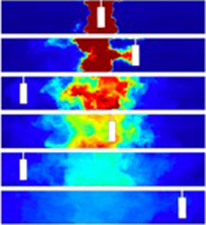
In figure 2(a), we present a series of images which were captured at different times during experiment k (see table 1). It is seen that a pulse of neutrally buoyant, dyed fluid was initially located in the centre of the tank, while the fluid at both sides was clear. Over time, the dyed fluid dispersed to both edges of the tank following multiple oscillations of the cylinder. Figure 2(b) presents these images in false colour using the calibrated light attenuation data, to help visualise the mixing. We observe that the periodic mixing caused by the oscillations of the cylinder results in the dye becoming increasingly well mixed vertically in the tank, with fluctuations in the vertical profile of dye concentration decaying to values of order 5 %–10 % or smaller relative to the mean after 2–3 oscillations of the cylinder. Figure 2(b) also shows that as the dye gradually spreads to the ends of the tank, its vertically averaged mean concentration progressively decreases. In figure 2(c), we present data from three experiments in which the cylinder speed was fixed, while its diameter was changed (experiments c, f and l in table 1). For each experiment, a time series of the vertically averaged dye concentration profiles along the channel is plotted using false colours. In each panel, the diagonal white lines correspond to the position of the cylinder as the experiment proceeds. It is seen that the dye migrates from the centre to the outer edge of the tank and its concentration decreases. After reaching the edge of the tank, the dye gradually becomes well mixed throughout the tank. Figure 2(c) also shows that with a larger cylinder, the mixing is faster: for example, compare the outcome of experiments c and l, in which the diameter of the cylinder was  $d=5$ and 2.5 cm, respectively.

Figure 2. (a) Series of images illustrating the dispersal of a pulse of dye during experiment k (see table 1). The images were captured at times 0, 16.3, 35.2, 45.9, 72.3 and 110.6 s after the beginning of the experiment. (b) For each image, false colours are used to illustrate the dye concentration field in the tank. (c) Time series of the vertically averaged profiles of dye concentration in the tank in experiments c, f and l (see table 1). In each time series image, the diagonal white line corresponds to the position of the cylinder at different times during the experiment.
For each image captured during an experiment, we have measured the centre of mass of dye in the tank,  $x_c$, defined by the relation
 \begin{equation} \int_{-L/2}^{x_c}\bar{c}\, \textrm{d} x=\int_{x_c}^{L/2}\bar{c}\, \textrm{d} x \quad \text{where } \bar{c}(x,t)=\frac{1}{H}\int_{0}^{H} c(x,y,t) \, \textrm{d} y. \end{equation}
 Using our estimates of  $x_c$, we have then calculated the variance of the position of the vertically averaged dye pulse as a function of time, $\sigma ^2$:
 \begin{equation} \sigma^2=\frac{\displaystyle\int_{-L/2}^{L/2} \bar{c}(x-x_c)^2 \, \textrm{d} x}{\displaystyle\int_{-L/2}^{L/2} \bar{c} \, \textrm{d} x}.\end{equation}
 In figure 3(a) we present data illustrating the variation of  $x_c/L$ as a function of $tu/L$ in experiments a–p (see table 1). The time scale $L/u$ corresponds to the time for the cylinder to traverse the length of the tank, with a corresponding frequency $f=u/L$. It is seen that the centre of mass of the dye is initially located near the centre of the tank, $x_c\approx L/2$ (figure 3a). However, as the cylinder moves across the pulse of dye, there is a net displacement of fluid in the tank, which is associated with the volume of the cylinder: this causes $x_c$ to be displaced by up to 3–4 cm during the initial oscillations when the dye is localised near the centre of the tank (figure 3a). However, as the dye becomes increasingly mixed along the tank, this fluctuation in the location of the centre of mass of the dye relative to the centre of the tank, which is associated with the oscillations, becomes much smaller.

Figure 3. (a) Coordinate of the centre of mass of the dyed fluid,  $x_c$, as a function of time, $t$.
$t$.  $x_c$ has been estimated using (3.1). Data for experiments a–p (see table 1) are presented in dimensionless form: the coordinate of the centre of mass, $x_c$, is scaled by the length of the tank, $L$, while time $t$ is scaled by the time required for the cylinder to traverse the tank, $f^{-1}=L/u$.(b) Variance of the position of the dye pulse, $\sigma ^2$ (see (3.2)) at early times during the experiments. For clarity, only a selection of profiles have been plotted in this figure, while the collapse of all experimental results is presented in figure 5(b). (c) Root mean square deviation of the tracer concentration from the mean, $\eta$ (see (3.3)), at late times during the experiments. For clarity, only a selection of profiles have been plotted in this figure, while the collapse of all experimental results is presented in figure 7(b).
In figure 3(b) we illustrate the dependence of  $\sigma ^2$ as a function of time in a selection of the experiments from table 1. On the vertical axis, the variance is scaled by the speed of the cylinder, $u$, multiplied by the width of the channel, $W$, and time. A virtual time origin $t_0$ is used to account for the effective time which would be required for the dyed fluid to spread to the initial width of the dye pulse in the tank, as discussed in § 4. In figure 3(b) we can see that after a very early-time transient, the ratio $\sigma ^2/(uW(t+t_0))$ is approximately constant over time before the dye pulse has spread to the far walls of the tank (see the horizontal dotted lines in figure 3b). This suggests that for $tu/L<8-10$ approximately, the dye spreads along the channel as a diffusion-type process. It is seen that in each experiment, the ratio $\sigma ^2/(uW(t+t_0))$ tends to a different constant, and this suggests that the rate of spreading of the dye is controlled by additional parameters, such as the cylinder diameter $d$ or the channel length $L$: we will explore these dependencies systematically in § 4. The curves plotted in figure 3(b) exhibit a series of periodic fluctuations which are associated with the cylinder motion. In fact, as noted in § 2, the linear interpolation of the dye concentration field in the region occupied by the opaque cylinder introduces small, systematic variations in which $\sigma$ increases and then decreases as the cylinder passes through the pulse of dyed fluid in the tank. However, it is seen in figure 3(b) that these fluctuations do not affect the mean values of $\sigma ^2$ averaged over a number of oscillations of the cylinder. We note that towards the end of each of the data sets shown in figure 3(b), the variance begins to decrease from the constant value, and this corresponds to the point at which the spreading of the dye is suppressed by the end walls of the tank.
At later times during each experiment, when the dye extends across the whole length of the tank, we have measured the root mean square deviation of the tracer concentration from the along-channel mean,  $\bar {\bar {c}}$, to quantify the progressive homogenisation of the dye concentration throughout the tank
 \begin{equation} \eta=\frac{1}{HL\bar{\bar{c}}}\int_{-L/2}^{L/2}\int_{0}^{H}\lvert {\bar c(x,t)} -\bar{\bar{c}}\rvert \, \textrm{d} y\, \textrm{d} x \quad \text{where } \bar{\bar{c}}=\frac{1}{HL}\int_{-L/2}^{L/2}\int_{0}^{H}c \, \textrm{d} y\, \textrm{d} x.\end{equation}
 In figure 3(c) we show the variation of  $\ln (\eta )$ with time for a selection of the experiments in table 1. Dotted straight lines are plotted besides each curve, illustrating how for $tu/L>15\text {--}20$, $\eta$ decays approximately exponentially with time, with small periodic fluctuations associated with the oscillations of the cylinder in the tank.
4. Dimensional analysis and scaling laws
The data presented in figure 3 suggest that there is an early-time phase in which the lateral extent of the tracer increases with time at a rate dependent upon  $t^{1/2}$, followed by a phase in which the concentration becomes progressively more uniform along the channel, adjusting to this state exponentially. However, the multiplicative constant varies from experiment to experiment. We now seek to develop some scaling laws for these constants using a series of systematic experiments. We expect that the dye will spread along the corridor as a dispersion-type process as the wake mixes the tracer back and forth and so has no net directionality. At early times, this would be consistent with a law of the form
 \begin{equation} \sigma = (D(t+t_0))^{1/2},\end{equation}
where  $D$ is an effective dispersivity with dimensions $[L^2/T]$ and $t_0$ is the time required for the tracer to disperse from a virtual point source to the initial finite length of the dye pulse in the tank at the start of the experiment, with the initial standard deviation given by
 \begin{equation} \sigma_0=(Dt_0)^{1/2}.\end{equation}
 For each experiment we have estimated  $t_0$, and we have found it to be of order 10–20 s, depending on the width of the dye pulse at the beginning of each experiment (see figure 3b). This is typically less than 10 %–15 % of the time required for $\sigma$ to reach the end walls of the tank, with the exception of the few experiments in which the length of the channel was reduced (experiments e, g, h in table 1), for which the correction was of order 20 %–30 %.
The stirring and mixing of the tracer is achieved by the wake of the cylinder, and so we expect that  $D$ scales with the product of the speed and radius of the cylinder; however, it may also be a function of the ratio of the channel width to the cylinder diameter (cf. Williamson Reference Williamson1996). In order to explore this, we now analyse the experimental results in a systematic fashion, varying the speed and the diameter of the cylinder, and the width and length of the channel, in each case while keeping other parameters fixed. Since the speed of the cylinder is the only parameter which includes time in its dimensions, by dimensional analysis we expect that
 \begin{equation} D = uW\mathcal{F}\left(\frac{d}{W}, \frac{L}{W}\right),\end{equation}
where  $\mathcal {F}$ is a function of the ratio of the diameter of the cylinder to the width of the channel, $d/W$, and the length to the width of the channel, $L/W$. In figure 4(a), we use the results of four experiments in which $u$ changes but everything else is fixed (experiments a, b, d and j, see table 1), and show that the ratio $\sigma /(uW(t+t_0))^{1/2}$ is approximately constant, with variations of less than 3 %, indicating that $\mathcal {F}$ is independent of $u$ as expected. Motivated by the experimental results, we propose that $\mathcal {F}$ may be given by the product of a function $\mathcal {F}_1(d/W)$ multiplied by a separate function $\mathcal {F}_2(L/W)$
 \begin{equation} \mathcal{F}\left(\frac{d}{W}, \frac{L}{W}\right)=\mathcal{F}_1\left(\frac{d}{W}\right)\times\mathcal{F}_2\left( \frac{L}{W}\right).\end{equation}
Figure 4. Effects of: (a) the speed of the cylinder,  $u$; (b) the ratio of the width of the cylinder to that of the channel, $d/W$; and (c) the ratio of the width to the length of the channel, $W/L$, on the dispersivity of the tracer in the channel.
In figure 4(b), we show the variation of  $\mathcal {F}_1$ as a function of $d/W$, for a series of experiments in which everything other than $d$ is fixed (experiments c, f, i, k, l, m, n, o and p, see table 1). Within experimental error, $\mathcal {F}_1$ is found to increase linearly with the ratio $d/W$,
 \begin{equation} \mathcal{F}_1(d/W) =(0.26\pm0.03) (d/W),\end{equation}
indicating that the diffusion of the tracer is enhanced when the diameter of the cylinder is increased (see figure 2c). Assuming that (4.5) captures the dependence of  $\mathcal {F}$ on the dimensionless group $d/W$, we have rescaled all data from experiments a–p in table 1 to explore the variation of $D$ as a function of $L/W$. In figure 4(c), we illustrate the variation of $\sigma ^2/(uL(t+t_0)\mathcal {F}_1)$ as a function of $L/W$ and obtain
 \begin{equation} \mathcal{F}_2(L/W)=(9.2\pm0.8) (L/W)^{-1}.\end{equation}
 In figure 4(c) there is some variation in  $\sigma ^2/(uL(t+t_0)\mathcal {F}_1)$ for $W/L=0.11$: here, each point corresponds to an experiment with a different value of $d/W$ (see table 1); however, it is seen that the estimate given by (4.6) (dashed line) lies within 10 % of each data point.
Based on all the experiments, we therefore propose the approximate empirical law
 \begin{equation} D_{model} =(2.4\pm0.5)\frac{udW}{L},\end{equation}
leading to the approximate relation
 \begin{equation} \frac{\sigma}{L} = (1.55\pm0.16)\left(\frac{udW(t+t_0)}{L^3}\right)^{{1}/{2}}.\end{equation}
 This is consistent within an error of less than 10 % with all our data, as illustrated in figure 5(a), where we compare  $D$ as measured from the results of experiments a–p in table 1 with the model approximation given by (4.7). As a further test, in figure 5(b) the model is used to rescale and collapse the standard deviation profiles of the tracer distribution, $\sigma /L$, as a function of $(D_{model}(t+t_0))^{1/2}/L$. It is seen that the model provides a good fit to all the data.

Figure 5. (a) Comparison of the values of  $D$ estimated using (4.7) for experiments a–p (see table 1) with the values measured during the experiments; (b) illustration of the rescaled standard deviation of the tracer distribution at early times during experiments a–p (see table 1), as a function of the rescaled time.
If the mixing produced by the cylinder is dispersive in nature, as indicated by this early time behaviour of the standard deviation, then we expect the ensemble average of the concentration, averaged across each cross-sectional area,  ${\bar c}(x,t)$ to be governed by a turbulent diffusion equation of the form
 \begin{equation} \frac{\partial {\bar c} }{\partial t} = D \frac{\partial^2 {\bar c} }{\partial x^2}.\end{equation}
At early time, the evolution of the concentration of a pulse of tracer is therefore expected to follow a solution of the form
 \begin{equation} {\bar c}(x,t) = \frac{ K }{(4{\rm \pi} D(t+t_0))^{1/2}} \exp \left( - \frac{(x-x_c)^2}{4D(t+t_0)}\right), \end{equation}
where  $x_c$ is the position of the centre of the dye pulse (see (3.1)), and where $K = \int _{-L/2}^{L/2} \bar {c}(x,o) \, \textrm {d} x$, evaluated at the start of the experiment. In figure 6 we consider experiments a–p (see table 1) and show the variation of the profile $c(x,t) (4{\rm \pi} D(t+t_0))^{1/2}/K$ as a function of $(x-x_c)/(4D(t+t_0))^{1/2}$, and we compare this with the above solution. For each experiment, we have taken the vertically averaged dye concentration profiles along the channel as measured at 20 different times during the experiment and we plot $c(x,t)(4{\rm \pi} D(t+t_o))^{1/2}/K$ as a function of $(x-x_c)/(4D(t+t_o))^{1/2}$ (an example is given from experiment m in figure 6a). We then take the time average of these profiles (red dashed line in figure 6a) for each experiment, and in figure 6(b) we compare these averages from each experiment with the model solution. It is seen that there is a fractional error of less than 5 % between the model Gaussian (equation 4.10) and the average concentration profile from each experiment, suggesting that the dispersive model of mixing provides a satisfactory description of the data.

Figure 6. (a) A series of 20 dye concentration profiles as measured at regular time intervals between times  $t_1=10$ s and $t_2=70$ s during experiment m (see table 1) are collapsed using (4.10). The mean curve resulting from the average of the collapsed profiles is plotted using a dashed red line. (b) Comparison of the average collapsed profiles calculated for experiments a–p (see table 1). The profiles are compared with the Gaussian distribution plotted using (4.10) (red dashed line). It is seen that there is an error of less than 5 % between the averaged profiles and the Gaussian curve.
The initial spreading of the dye given by (4.10) becomes limited by the end walls of the tank when the dye reaches them. As a simple estimate, this transition occurs when  $t = L^2/2D = L^3 / (4.8 udW)$, after which the dispersion of the tracer becomes limited by the no-flux condition through the end walls, and this leads to a gradual homogenisation of the dye concentration in the channel. The adjustment of the dye to a uniform concentration can then be described by a power series solution for the diffusion (4.9) of the form
 \begin{equation} \bar{c}(x, t)=\bar{\bar{c}}+\sum_{n=1}^\infty a_n \exp\left(-\frac{4{\rm \pi}^2 D n^2(t+t_0)}{L^2}\right)\cos\left(\frac{2{\rm \pi} n x }{L}\right),\end{equation}
where  $\bar {c}(x, t)$ is the vertically averaged dye concentration profile along the channel (see (3.1)), $\bar {\bar {c}}$ is the mean concentration of dye in the channel (see (3.3)) and the coefficients $a_n$ depend on the initial distribution of the dye. The slowest decaying mode in this power series solution is proportional to
 \begin{equation} \exp\left( - \frac{4{\rm \pi}^2 D (t+t_0)}{ L^2}\right) \cos\left( \frac{2 {\rm \pi}x}{ L}\right).\end{equation}
Therefore, at long times, when only the slowest decaying mode is significant, we expect  $\eta$ to decay according to the relation
 \begin{equation} \ln(\eta(t)) = A-\frac{4{\rm \pi}^2 D (t+t_0)}{ L^2},\end{equation}
where  $A$ is a constant dependent on the coefficient $a_1$ in the power series solution. In order to test this prediction, we have estimated the value of $D$ for each of experiments a–p (see table 1) from the slope of the curves in the log–linear plot shown in figure 3(c). By following a similar exercise to that above, which led to (4.7), we find that using this long time estimates for $D$, the data can be collapsed to the empirical law $D_{\eta } = (2.66\pm 0.4)\, udW/L$, which, within the error bars, coincides with the prediction for $D$ based on the early-time data given in (4.7). To illustrate the overlap of these diffusivities, in figure 7(a) we include a plot which compares $D$ with $D_{\eta }$. Furthermore, in figure 7(b), we use the time scale $\tau =L^2/(4{\rm \pi} ^2D)$ as a scaling for the adjustment time, and we show the variation of $\ln (\eta )-A$ as a function of this rescaled time, $t/\tau$. It is seen that all the experimental data converge to a straight line.

Figure 7. (a) The estimate of the diffusion coefficient  $D$ (m $^2$ s $^{-1}$) obtained from the early-time variance data (experiments a–p in table 1, see figure 4) is compared with that obtained from the late-time data, $D_{\eta }$ (m $^2$ s $^{-1}$, see figure 3c and (4.12) and (4.13)). (b) Illustration of the rescaled profiles of root mean square deviation of tracer concentration from the mean, $\eta$ (see figure 2c). The collapse of the profiles from experiments a–p (see table 1) is plotted using (4.13).
5. Effect of the frequency of walkers
In order to apply this model to a real situation in which there may be a variable number of people walking along the corridor as a function of time, we need to include a further dependence in the model for  $D$. To this end, we repeated some of the experiments but at the end of each traverse of the tank, the cylinder was paused for a fixed period of time and then resumed (experiments q–v, see table 1). An image of the mixing produced by these experiments is shown in figure 8(a). In order to model the dispersion in these experiments, we need to account for the smaller frequency of oscillations. The present model includes an implicit frequency $f = u/L$, corresponding to the number of traverses of the cylinder along the length of the tank per unit time, resulting in a period $t_t = L/u$. If the cylinder stops for a time $t_s$ at the end of the tank, then the frequency of oscillations reduces by the fraction
 \begin{equation} \hat{t}=\frac{t_t}{t_t+t_s}.\end{equation}
Figure 8. (a) Time series of the vertically averaged profiles of dye concentration in the tank in four experiments with decreasing frequency of cylinder oscillation in the tank (experiments f, r, t and v, see table 1); (b) collapse of the standard deviation profiles of the tracer distribution in the channel using the rescaled diffusion coefficient given by (5.2) (experiments f and q–v, see table 1).
In the experiments, visual observation suggests that the wake decays over a time comparable to a few multiples of the cylinder radius divided by the cylinder speed. Given that the delay between successive passes of the channel is relatively long compared to this decay time, then we expect that the dispersion  $D$ should be rescaled to the new frequency of passage of the cylinder, giving a dispersion coefficient
 \begin{equation} D_f = \hat{t}D.\end{equation}
 In figure 8(b) we illustrate that this revised value  $D_f$ can be used to describe the growth of the standard deviation $\sigma /L$ for a series of experiments which include time delays $t_s=2.7$, 4.5, 6.0, 8.8, 10.0 and 12.3 s (experiments q–v, see table 1), suggesting that the dispersion coefficient presented in (4.7) can be written in the form
 \begin{equation} D_f = (2.4\pm0.5) fdW,\end{equation}
where  $f$ is the average frequency of the cylinder moving along the corridor, $W$ is the width of the corridor traversed by the cylinder and $d$ the cylinder diameter.
6. Discussion
The simplified model experiments presented in this paper suggest that for  $0.15<d/W<0.5$, the motion of a cylinder in a channel leads to a dispersion coefficient $D = (2.4\pm 0.5) fdW$, and that the associated diffusion equation models the transport of tracer by the oscillatory motion of a cylinder along the channel, with no net flow.
In a corridor in a busy hospital or public building, we expect  $f$ to lie in the range $0.01<f<0.1\ {\rm s}^{-1}$, and so with typical corridor widths of order $W\approx 2\text {--}3$ m (National Health Service 2013) and typical people widths of order $d\approx 0.4\text {--}0.5$ m, the magnitude of this dispersive transport $D$ is expected to be of order $0.01\text {--}0.1$ m $^2$ s $^{-1}$. It is worth noting that this is of order 1 to 10 larger than the typical effective diffusion coefficients associated with the ventilation flow inside a room, $D_v\approx 10^{-3}{-}10^{-2}$ (see § 1, cf. Nicas Reference Nicas2009; Cheng et al. Reference Cheng, Acevedo-Bolton, Jiang, Klepeis, Ott, Fringer and Hildemann2011; Shao et al. Reference Shao, Ramachandran, Arnold and Ramachandran2017; Foat et al. Reference Foat, Drodge, Nally and Parker2020); this highlights the very significant role that people moving through a space can have in mixing the air and airborne aerosols. Given that aerosols of size 5–10 $\mathrm {\mu }$m will remain suspended for times in excess of 100–1000 s, we expect them to be mixed over distances of order $(Dt)^{1/2} =1.5\text {--}15$ m from the original source; the aerosols will be continually diluted across this region. This mixing will delay the time for removal of the aerosols by the ventilation flow. Corridors are rarely considered in planning airborne infection control strategies, yet our study shows that the movement of people in corridors may play a significant role in transporting aerosol around a building. Similar dispersive effects are likely to occur within rooms. Going forward, we plan to extend this work to consider the mixing by people moving in fully three-dimensional spaces, as well as the small-aspect ratio corridors considered herein.
Declaration of interests
The authors report no conflict of interest.


 Open access