


Introduction
Climate change over the 21st century is expected to considerably accelerate the retreat of glaciers in the European Alps (e.g. Reference Schneeberger, Blatter, Abe-Ouchi and WildSchneeberger and others, 2003; Reference Zemp, Haeberli, Hoelzle and PaulZemp and others, 2006; Reference SolomonSolomon and others, 2007). Prediction of the future extent of Alpine glaciers is of major interest, due to their regulating effect on the hydrological cycle (Reference HuntingtonHuntington, 2006), their economic importance (tourism, hydropower production), their link with different types of natural hazards (e.g. Reference Werder, Bauder, Funk and KeusenWerder and others, 2010) and their potential to raise the global eustatic sea level (Reference Kaser, Cogley, Dyurgerov, Meier and OhmuraKaser and others, 2006).
Since the end of the Little Ice Age in the mid-19th century, Alpine glaciers have receded significantly due to a marked temperature increase (Reference Haeberli and BenistonHaeberli and Beniston, 1998). However, the response of their terminus position, as well as the glacier surface mass balance, shows a nonuniform pattern (e.g. Reference Huss, Hock, Bauder and FunkHuss and others, 2010; Reference Lüthi, Bauder and FunkLüthi and others, 2010). Whereas small glaciers have a short response time and adapt rapidly to changed climate conditions, large glaciers dampen climatic fluctuations on the decadal scale and retreat more smoothly. Thus, voluminous glaciers such as Grosser Aletschgletscher – by far the largest glacier in the European Alps – are valuable indicators of long-term climate trends, since they are almost insensitive to short-term swings, such as those that caused many small glaciers in the Alps to advance in the 1920s and 1980s (Glaciological reports, 1881–2009).
A number of comprehensive three-dimensional (3-D) numerical models for the computation of the ice flow and surface evolution of valley glaciers have been developed during the past decade. Some of the models used the first-order approximation (Reference BlatterBlatter, 1995) for the ice-flow computation (e.g. Reference AlbrechtAlbrecht, 2000; Reference Schneeberger, Albrecht, Blatter, Wild and HockSchneeberger and others, 2001, Reference Schneeberger, Blatter, Abe-Ouchi and Wild2003). More recently, the 3-D full Stokes equations have become more viable in the field of mountain glacier modelling for several reasons (e.g. Reference Zwinger, Greve, Gagliardini, Shiraiwa and LylyZwinger and others, 2007; Reference Jouvet, Picasso, Rappaz and BlatterJouvet and others, 2008, Reference Jouvet, Huss, Blatter, Picasso and Rappaz2009; Reference Zwinger and MooreZwinger and Moore, 2009). First, shallow models may be deficient at describing complex ice flow over sloping bedrock (Reference Le Meur, Gagliardini, Zwinger and RuokolainenLe Meur and others, 2004). Second, the Stokes numerical implementation using finite-element methods is well known (Reference Ern and GuermondErn and Guermond, 2004) and can be performed using external open-source or commercial codes. Third, the performance of standard computers allows the Stokes problem to be solved with high resolution and within reasonable computational time.
Over the past 20 years, glacier prognostics have been a subject of growing interest (Reference OerlemansOerlemans and others, 1998). Specific studies of the future retreat of Alpine glaciers have been performed, for example for Griesgletscher (Reference AlbrechtAlbrecht, 2000), Rhonegletscher (Reference Wallinga and van de WalWallinga and Van de Wal, 1998; Reference Jouvet, Huss, Blatter, Picasso and RappazJouvet and others, 2009) and Glacier de Saint-Sorlin (Reference Le Meur, Gerbaux, Schäfer and VincentLe Meur and others, 2007). In order to link the ice-flow models with climatic changes, a wide range of mass-balance models have been considered. For instance, Reference Wallinga and van de WalWallinga and Van de Wal (1998) use a simple parameterization that relies on the annual temperature at the equilibrium-line altitude (ELA), whereas Reference Giesen and OerlemansGiesen and Oerlemans (2010) use an energy-balance formulation to drive an ice-flow model for Hardangerjøkulen, Norway, over the 21st century.
Here ice is treated as an incompressible, isothermal and viscous fluid, and basal sliding is included. The 3-D numerical model is based on a volume of fluid formulation to describe the domain of ice (Reference Jouvet, Picasso, Rappaz and BlatterJouvet and others, 2008). This model combines the finite-element method to solve the full Stokes equations and the method of characteristics to compute the time evolution of the volume of fluid. Digital elevation models (DEMs) of the bedrock and of the ice thickness are used to mesh and initialize the glacier geometry. Glacier surface mass balance is calculated in daily time-steps using a distributed accumulation and temperature-index melt model (Reference HockHock, 1999). Using meteorological data, the evolution of Grosser Aletschgletscher since 1880 is simulated and compared to measurements. Future retreat of Grosser Aletschgletscher, and other nearby glaciers, is modelled based on eight different climate scenarios. Regional climate-model results from the ENSEMBLES project (Reference Van der Linden and MitchellVan der Linden and Mitchell, 2009), a simple temperature increase referring to the ‘two degree target’ and climate conditions in several periods in the past are considered to perform simulations for the period 2000–2100. In the last part of the paper, we analyse the influence of the spatio-temporal changes in supraglacial debris on the rate of glacier retreat.
Data and Field Observations
Grosser Aletschgletscher consists of three large accumulation basins merging into a long and curved tongue at Konkordiaplatz (Fig. 1). In 1999 Grosser Aletschgletscher had a length of ∼22 km and an area of 83 km2 (Reference Bauder, Funk and HussBauder and others, 2007). The volume of Aletschgletscher was roughly 15 km3 in 1999, representing ∼20% of the entire ice volume in Switzerland (Reference Farinotti, Huss, Bauder and FunkFarinotti and others, 2009). Its ice thickness reaches >800 m at Konkordiaplatz. Since 1880 the terminus position of Aletschgletscher has retreated by 2.8 km (Glaciological reports, 1881–2009). The glacier has lost an ice volume of >5 km3 (Reference Bauder, Funk and HussBauder and others, 2007), corresponding to about one-quarter of its initial volume. This study includes two other medium-sized glaciers on the east side of Grosser Aletschgletscher (Oberaletschgletscher and Mittelaletschgletscher) and some smaller glaciers (Fig. 1). Thus, the entire glacier cluster in the drainage basin of Aletschgletscher is modelled.

Fig. 1. Overview map of Grosser Aletschgletscher and smaller glaciers in the drainage basin. Glacier outlines and surface contours (200 m interval) refer to the year 1999. The shading indicates the ice thickness. The dashed line shows the central flowline. Black dots indicate the location of velocity measurements. The solid contour at the confluence of three glaciers at Konkordiaplatz shows the upper limit of the zone where basal sliding is considered.
A wide range of field data is available for the study site:
-
Five DEMs were derived either from topographic maps (1880, 1926, 1957) or from aerial photographs (1980, 1999) (Reference Bauder, Funk and HussBauder and others, 2007). The DEMs have a resolution of 50 m, and an accuracy of ±3–5 m (first two DEMs) and ±0.3–1 m (last three DEMs).
-
In April 1995 several radio-echo sounding profiles were compiled to determine the ice thickness. As most of the profiles did not reach the lowest parts of the glacier bed they were reinterpreted by Reference Farinotti, Huss, Bauder and FunkFarinotti and others (2009), using a method to estimate distributed ice thickness based on an inversion of surface topography. As a result, a complete bedrock map of the entire glacier now exists which agrees with field data, where available.
-
Point-based surface mass balance was measured on Grosser Aletschgletscher for several decades. One measurement site has existed near Jungfraujoch in the accumulation area with continuous mass-balance data since 1920 (Reference Huss, Funk and OhmuraHuss and others, 2009). Additionally, mass balance was measured annually at several dozen stakes located on the tongue between the mid-1940s and the early 1980s. At some stakes, readings in winter, including snow pits, were performed in order to determine the snow accumulation.
-
Accurate coordinates derived from theodolite-based trigonometry are available for all stakes. These annual displacements between reported period lengths of ∼1 year were used to calculate annual ice-flow velocities. As the stakes on the tongue of Grosser Aletschgletscher were arranged in clusters (Fig. 1), flow velocities for each cluster and all years of measurements (about 1950–80) were averaged for easier comparison with the model results.
-
Monthly discharge measurements since 1923 are available from a gauging station near the glacier tongue.
-
Different meteorological time series documented the changes in climatic conditions during the 20th century. We used the homogenized daily temperatures recorded since 1864 at Sion (Reference Begert, Schlegel and KirchhoferBegert and others, 2005) and daily precipitation sums from Lauterbrunnen to drive the mass-balance model.
Methods
In this section, the symbols ‘, i’ and ‘, j’ denote the space derivative with respect to the ith and jth spatial components while the ‘dot above’ symbol denotes the time derivative.
Ice-flow model
Ice is considered to be an incompressible non-Newtonian fluid. The constitutive law for the ice flow is given by the regularized Glen’s law (Reference GlenGlen, 1958; Reference Greve and BlatterGreve and Blatter, 2009):
where εij = (ui, j + uj,i)/2 are the components of the strain-rate tensor, ui are the velocity components, ![]() are the components of the deviatoric stress tensor, σij
are the components of the stress tensor, τ
II is the second invariant of τ defined by
are the components of the deviatoric stress tensor, σij
are the components of the stress tensor, τ
II is the second invariant of τ defined by ![]() , A is the rate factor, n is Glen’s exponent and τ
0 ≥ 0 is a regularization parameter. Note that ice effective viscosity, μ, defined by Equation (1) and the linear relation
, A is the rate factor, n is Glen’s exponent and τ
0 ≥ 0 is a regularization parameter. Note that ice effective viscosity, μ, defined by Equation (1) and the linear relation
is a function of ε which remains finite at zero when τ 0 > 0 but becomes infinite when τ 0 = 0, i.e. as in the original Glen’s law. In all simulations, we set n = 3 (Reference GudmundssonGudmundsson, 1999), the regularization parameter is fixed to τ 0 = 0.031 MPa and the rate factor, A, is calibrated with observed surface flow velocities. In practice, ice is so viscous that inertial and acceleration effects can be neglected. As a consequence, the equations expressing mass and momentum conservation for an incompressible material are reduced to the stationary Stokes equations:
where p is the internal ice pressure, ρ is the ice density and gi represents the components of the gravity force. The ice is assumed to be isothermal, as records of englacial temperature (Reference LaternserLaternser, 1992; Reference Suter, Laternser, Haeberli, Frauenfelder and HoelzleSuter and others, 2001) show that Grosser Aletschgletscher is temperate, except for limited areas above 4000 m a.s.l.
Boundary conditions
No force is exerted on the free glacier surface,
where ni represents the components of the outward-pointing unit vector. At the bedrock interface, both slip and no-slip conditions are applied in different parts of the glacier. Modelling subglacial sliding is difficult since it depends on many factors (e.g. the roughness of the bedrock, the subglacial water pressure and the ice temperature (Reference WeertmanWeertman, 1957; Reference FowlerFowler, 1986; Reference Vieli, Funk and BlatterVieli and others, 2000; Reference SchoofSchoof, 2005)). The effective pressure – the difference between ice and water pressure – plays a major role in the sliding processes (Reference SchoofSchoof, 2010), but is hard to evaluate since it is driven by many factors that change rapidly with time. For this reason, the water pressure is expected to strongly fluctuate over short timescales (Reference Fischer and ClarkeFischer and Clarke, 1997), thus hampering the application of parameter calibration procedures. The complexity of such phenomena motivates us to focus on a simpler model that is independent of the effective pressure. Glacier sliding occurs mainly when basal ice is at the melting temperature or when meltwater reaches the bedrock. As a consequence, less sliding is expected in the highest regions of the glacier, where meltwater production decreases. Based on this simple consideration, bedrock is divided into two parts by the altitude, z l, of the bedrock. Sliding is only considered below z l. Above z l, ice is assumed to be fixed to the bedrock and we have the condition
for i = 1, 2, 3, while below z l we consider the following empirical Weertman’s sliding law (Reference WeertmanWeertman, 1957; Reference HutterHutter, 1983):
where u b is the basal sliding velocity, τ b is the basal shear stress and c is a sliding coefficient. The sliding threshold altitude is set to a bedrock elevation of z l = 2400 m a.s.l. Thus, the sliding area contains the entire glacier tongue and Konkordiaplatz (Fig. 1). The sliding coefficient, c, is calibrated with observed surface ice-flow velocities.
Volume of fluid function
The domain of ice is described by a Eulerian formulation that allows all changes in topology to be taken into account. Following Reference Maronnier, Picasso and RappazMaronnier and others (2003) and Reference Jouvet, Picasso, Rappaz and BlatterJouvet and others (2008), we define the volume of fluid function, taking the value ‘1’ inside the glacier and ‘0’ outside. This function, denoted φ, is defined in a large box which contains the entire glacier and its near environment. A local mass balance along the ice/air interface yields the transport equation,
where b is the mass-balance function and bδ S is a source term acting on the ice/air interface.
Numerical model
The numerical method was presented in detail by Reference Jouvet, Picasso, Rappaz and BlatterJouvet and others (2008, Reference Jouvet, Huss, Blatter, Picasso and Rappaz2009), and we recall the main outlines of the method here. A decoupling algorithm allows Equations (3), (4) and (8) to be solved using different numerical methods.
First, the nonlinear Stokes problem, Equations (3) and (4), with boundary conditions Equations (5), (6) and (7), is solved on a fixed, unstructured mesh consisting of tetrahedrons. At each time-step, the problem nonlinearities due to Glen’s law and to the sliding law are solved using a fixed-point iteration method. For this purpose, we use a relationship between the viscosity and the strain rate obtained by combining Equations (1) and (2), the stress being eliminated. More precisely, for a given strain rate, the viscosity is obtained by solving an nth-order polynomial equation. For each fixed-point loop, we use the strain rate obtained in the previous iteration and find the viscosity using Newton’s method. The fixed-point method is even simpler in the case of nonlinear sliding, since Equation (7) can be inverted, i.e. the tangential stress is explicitly computable using the velocity obtained in the previous iteration. In practice, fewer than ten iterations are sufficient to reach convergence (Reference JouvetJouvet, 2010). At each fixed-point iteration, the linear Stokes problem is solved using a continuous, piecewise linear stabilized finite-element method (Reference Franca and FreyFranca and Frey, 1992).
Second, the transport equation, Equation (8), is solved on a fixed, regular grid of smaller cells covering the ice domain, using a forward method of characteristics (Reference Maronnier, Picasso and RappazMaronnier and others, 2003; Reference Jouvet, Picasso, Rappaz and BlatterJouvet and others, 2008). Since the volume of fluid is a discontinuous function across the ice/air interface, numerical diffusion must be reduced as much as possible. For this purpose, a post-processing procedure – a ‘simple line interface calculation’ method (Reference Scardovelli and ZaleskiScardovelli and Zaleski, 1999) – was performed. The transfer of data between the two meshes was performed by specific interpolation procedures (Reference Maronnier, Picasso and RappazMaronnier and others, 2003). First, the volume of fluid was interpolated from the structured grid to the unstructured mesh to determine the part of the unstructured mesh filled with ice to be considered for the new velocity calculation. Next, the velocities were interpolated on the structured grid to allow the transport step to be performed.
The method described combines the advantages of the finite-element method to treat the complex geometries of glaciers and the benefits of the volume-of-fluid method which is robust, mass-conserving and can take into account all changes in topology (Reference Jouvet, Picasso, Rappaz and BlatterJouvet and others, 2008).
Given the DEM of the bedrock, a surface mesh was generated by splitting each square into triangles in the same diagonal. In the same way, another surface mesh – that must exceed the surface of the glacier at any time – was generated by adding a safe distance of 250 m to the DEM surface elevation of year 1880, when the glacier was thickest. An unstructured mesh of tetrahedrons was generated between the two surfaces using the open-source mesher Gmsh (see Reference Geuzaine and RemacleGeuzaine and Remacle, 2009). To take into account the shallowness of the glacier, the mesh was refined along the vertical directional only. Final tetrahedrons were about 100 m long and 30 m high. The structured mesh was a large block made up of 20 m long cubes that entirely covered the unstructured mesh. With the meshes described above, the constant time-step of half a year proved to be optimal for the proposed method and the size of the considered glacier. All the computations were performed on an AMD Opteron 242 CPU with 4 GB memory. The CPU time required for performing a simulation over a period of ∼100 years ranged between 1 and 2 days. Most of the CPU time was consumed by the matrix-inversion steps for solving the Stokes equations; the time required to run the mass-balance model was negligibly small.
Mass-balance model
The mass-balance function, b, was obtained using a distributed accumulation and temperature-index melt model (Reference HockHock, 1999; Reference Huss, Bauder, Funk and HockHuss and others, 2008).
Below 3500 m a.s.l., precipitation is assumed to increase linearly with elevation (the rate is denoted G p). A correction factor, c prec, accounted for the gauge under-catch error of precipitation, and a threshold temperature of 1.5°C distinguished snow from rainfall (Reference HockHock, 1999). The spatial variation in accumulation over the glacier surface is substantially influenced by the preferential deposition of snow and snow redistribution. These effects were taken into account using a spatial snow distribution multiplier, D sn = D sn(x, y), derived from terrain characteristics (Reference Huss, Bauder, Funk and HockHuss and others, 2008). D sn also includes lateral precipitation gradients corresponding to the large-scale precipitation patterns obtained from a gridded precipitation dataset (PRISM; Reference Schwarb, Daly, Frei and SchärSchwarb and others, 2001). Snow accumulation Ac = Ac(x, y, t) at gridcell x, y and day t was calculated using the daily measured precipitation, P ws = P ws(t), at a nearby weather station:
where z = z(x, y) is the elevation of the glacier surface at gridcell x, y, z ws is the altitude of the weather station and T = T(x, y, t) is the daily mean air temperature extrapolated to the elevation, z(x, y), of each gridcell from the measured temperature assuming a linear temperature decrease with elevation.
Temperature-index models are based on a linear relation between positive air temperature and the melt rate. Here surface melt rates, M, were computed by
where f M is a melt factor, r ice/snow are radiation factors for ice and snow, T = T(x, y, t) is the air temperature extrapolated to each gridcell and I = I(x, y, t) is the clear-sky direct radiation (obtained from a DEM) that accounts for the effects of slope, aspect and topographic shading. Due to the empirical character of temperature-index models, the site-specific parameters, f M and r ice/snow, have to be calibrated using direct observations.
Optimal values for the three melt parameters, as well as the accumulation parameters (Equation (9)), have been obtained using a semi-automated calibration procedure with observed decadal ice volume changes of Grosser Aletschgletscher (1880–1999), and in situ measurements of accumulation and ablation at up to two dozen sites annually on the glacier surface over several decades (Reference Huss, Bauder, Funk and HockHuss and others, 2008). Annual glacier surface mass balance is defined as the sum of solid precipitation and snow- or ice melt at the end of the hydrological year (1 October–30 September).
Definition of climate scenarios
For model runs over the next 90 years we applied three types of climate scenario: (1) projected changes in air temperature and precipitation, based on regional climate models within the ENSEMBLES project (Reference Van der Linden and MitchellVan der Linden and Mitchell, 2009); (2) a simple linear temperature increase referring to the ‘two-degree target’ defined in the context of a political goal as the upper limit of global warming (Reference MeinshausenMeinshausen and others, 2009); and (3) mean climatic conditions observed in different periods in recent decades, fixed over the next 90 years. This strategy allows glacier changes to be assessed based on state-of-the-art climate projections that are, however, subject to considerable uncertainty. Transient glacier response in the next century was also evaluated using the well-defined climate conditions of the past.
The ENSEMBLES project (Reference Van der Linden and MitchellVan der Linden and Mitchell, 2009) consists of model chains of general circulation models (GCMs) coupled with regional climate models (RCMs). In total, four different GCMs were used to drive ten RCMs, providing a wide range of possible future changes in the climate system. All model runs are based on the SRES A1B emission scenario which assumes a future world of fast economic growth, global population that will peak mid-century and decline thereafter, and the rapid introduction of new and more efficient technologies (Reference Nakićenović and SwartNakićenović and Swart, 2000). The SRES A1B emission scenario also assumes a balance across all sources of energy. In this study, we use seasonally aggregated ‘delta change’ scenarios for Swiss meteorological stations derived from the ENSEMBLES dataset (Reference Bosshard, Kotlarski, Ewen and SchärBosshard and others, 2011). Daily changes in air temperature and precipitation relative to the period 1980– 2009 were generated for each of the ten RCMs for the 30 year time frames 2021–50 and 2070–99 for the Aletschgletscher region from Reference Bosshard, Kotlarski, Ewen and SchärBosshard and others (2011). In order to obtain transient changes over the 21st century, mean changes in the period were allocated to the years 2036 and 2085 (midpoints of the periods) and interpolated (extrapolated) linearly.
We considered three individual model scenarios out of the ten RCMs within the ENSEMBLES project. Air-temperature changes given by MPI-ECHAM-REMO are near the median of the ten RCMs in most seasons. SMHI-BCM-RCA describes a lower limit of air-temperature changes, and ETHZ-HadCM3Q0-CLM provides an upper limit of expected temperature changes for the A1B emission scenario. The three RCMs considered were driven by different GCMs, and are abbreviated as ENSmed, ENSmin and ENSmax in the following text. Expected temperature changes in summer are between +3.7°C and +7.7°C by 2100. Precipitation changes show a nonuniform pattern (Table 1). For each scenario, daily meteorological time series were generated by applying expected seasonal changes in air temperature and precipitation to detrended series recorded in randomly chosen years between 1900 and 2000.
Table 1. Deviation of mean annual air temperature, ΔTY, summer (June–August) temperature, ΔTS, and annual precipitation, ΔP, by 2100, from the period 1980–2009
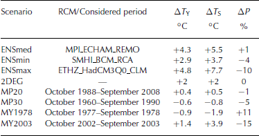
The scenarios from the ENSEMBLES project account for a rise in CO2 emissions that would follow technological development over the 21st century if there were no policy success in limiting emissions. Nevertheless, if CO2 emissions are halved by 2050 compared to 1990, global warming can be stabilized below two degrees (Reference MeinshausenMeinshausen and others, 2009). More than 100 countries have agreed the goal of a global warming limit of 2°C in order to limit the adverse effects of climate change. Based on this ‘two-degree target’, we define the simple scenario 2DEG, assuming a linear increase in air temperature by 2°C in all seasons by the year 2100 and no precipitation changes (Table 1).
By way of contrast to scenarios mimicking a changing climate, we define four additional scenarios that do not depend on any climate model that may be subject to considerable uncertainty and controversy. These scenarios are based on meteorological conditions from selected periods in the past. This allows the calculation of glacier extent in the (unlikely) case that the climate stabilizes on the mean of a given period in the past decades. The mid-1980s were characterized by a significant increase in air temperature and a reduction in snowfall events (Reference Begert, Schlegel and KirchhoferBegert and others, 2005; Reference MartyMarty, 2008), which caused a significant acceleration of glacier mass loss in the Alps (Reference Huss, Hock, Bauder and FunkHuss and others, 2010). Thus, we consider periods before and after this shift to analyse the response of Aletschgletscher to a prolongation of these climatic conditions. More precisely, scenario MP20 is generated by randomly picking annual meteorological series in the 20 year meteorological period 1989–2008. Another scenario (MP30) covers the conditions in the normal climatic period 1961–90.
To evaluate the effects of extreme years in the past, we consider two cases with strong deviations from the long-term mean. Scenario MY1978 is obtained by driving the model with air temperature and precipitation in the meteorological year 1978 (October 1977–September 1978), which resulted in the most positive annual mass balance of Aletschgletscher of the entire last century. Scenario MY2003 is based on the meteorological conditions during 2003 leading to an extremely negative mass balance of Alpine glaciers due to summer temperatures reaching an unprecedentedly high level (Table 1).
Results
Model calibration
Calibration of the rate factor, A, and the sliding coefficient, c, was based on the time-averaged surface velocities observed on the glacier tongue (Fig. 1). Since surface displacement had been measured approximately over the period 1950–80, we computed the stationary velocity fields for the years 1957 and 1980, for which DEMs were available, using different couples of parameters. Computed velocities between 1957 and 1980 changed less than 10 m a− 1, and were averaged for comparison. For several realistic rate factors, we determined the sliding coefficient that minimized the root mean square (rms) between computed and measured velocities (Table 2).
Table 2. Optimal sliding coefficients, c, for several rate factors, A. For the highest and lowest of the five measurement locations displayed in Figure 1, measured and computed surface velocities, computed basal velocities (m a−1) and sliding fraction (basal velocity divided by surface velocity) are indicated for each parameterization. The root mean square (rms) between measured and simulated surface velocity is given
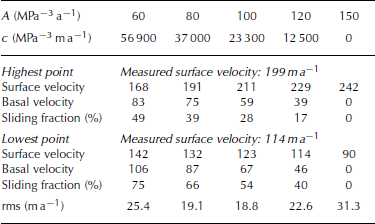
Among the combinations of coefficients given in Table 2, we use in what follows, the one that minimizes the rms, i.e. parameters (A, c) = (100, 23 300). Interestingly, this optimal couple results in a balanced contribution of sliding and ice deformation to surface velocities at the lowest point on the glacier tongue, but the sliding contribution decreases to 28% immediately below Konkordiaplatz (Table 2). Note that, if no sliding is accounted for (i.e. c = 0), then A = 150 MPa−3 a−1 is the optimal rate factor, which is significantly higher than indicated by field studies (Reference GudmundssonGudmundsson, 1999). In that case, the rms = 31.3 m a− 1 is maximal (Table 2). From this experiment we conclude that sliding effects on the glacier tongue need to be accounted for in order to correctly reproduce the observed surface velocity field.
The coefficients of the mass-balance model are calibrated according to observed ice volume changes, in situ point-based seasonal mass-balance measurements and discharge at the glacier snout (Reference Huss, Bauder, Funk and HockHuss and others, 2008). As a result, accumulation parameters involved in Equation (9) are G p = 3.5 × 10− 4 and c prec = 1.25. Melt parameters involved in Equation (10) are fine-tuned for each period between two subsequent DEMs. For the period 1980–99, we obtain f M = 1.78 × 10− 3 m d−1 °C− 1; r ice and r snow are set to 2.14 ×10− 5 and 1.60 ×10− 5 m3 W−1 d−1°C− 1, respectively.
20th-century retreat
Here we evaluate the performance of the model by comparing the simulated changes in glacier surface elevation with repeated DEMs throughout the 20th century. The calculations were initiated employing the first accurate DEM in 1880, and the evolution of Grosser Aletschgletscher was simulated until 1999. The two smaller glaciers (Oberaletschgletscher and Mittelaletschgletscher) were excluded from this model run as no topographies for model initialization in 1880 were available. The DEMs for 1929, 1957, 1980 and 1999 were used for validation.
Simulated and observed changes in ice volume agree well (Fig. 2). However, when comparing glacier terminus retreat along the central flowline (Fig. 1), the modelled retreat rate is too high for the last 50 years (Fig. 2, solid line). This disagreement can be attributed mainly to an inaccurate description of basal sliding in the model, resulting in a too-slow ice-flow regime at the glacier tongue. Thus, glacier retreat is overestimated by ∼500 m over the last five decades. Longitudinal profiles of simulated glacier surface elevation are compared with DEMs (Fig. 3). The model slightly underestimates the surface elevation on the glacier tongue and overestimates it in the accumulation area. The model performance is assessed by evaluating the rms of the difference between observed and modelled surface elevation over the entire glacier. The rms values are 32, 34, 34 and 33 m for the years 1926, 1957, 1980 and 1999. Considering the size of Grosser Aletschgletscher and the resolution of the structured grid (20 m), these results are satisfying. The disagreements can be attributed mainly to the description of basal sliding. Other factors potentially explaining the disagreements are: (1) the ice-flow model may not have described glacier dynamics correctly, (2) the bedrock elevation may have been inaccurate in some regions of the glacier and (3) uncertainties in the mass-balance model.

Fig. 2. Modelled glacier length and ice volume of Grosser Aletschgletscher from 1880 to 1999. Length was calculated along the central flowline (Fig. 1). Observed volumes and lengths were obtained from DEMs and are indicated by crosses. Model results for parameterizations (A, c) = (80,37 000) and (A, c) = (100, 23 300) are represented by dotted and solid lines, respectively.

Fig. 3. Observed and calculated surface elevation along a longitudinal profile of Grosser Aletschgletscher in 1926 and 1999.
Sensitivity to ice-flow parameters
The ice-flow parameters, A and c, were tuned to observed surface velocities using two glacier geometries given by DEMs. In order to evaluate the impact of this calibration procedure on long-term glacier evolution, the model was run over the 20th century also using the parameterization (A, c) = (80, 37 000) that fits measurements almost as well as the optimal couple (A, c) = (100, 23 300) (Table 2). Figure 2 indicates that the ice volumes over the 20th century agreed well for both parameterizations. The difference is <2% by 1999. Glacier length, however, is better reproduced by (A, c) = (100, 23 300), even if the difference between the two parameterizations remains small (100–500 m). This additional experiment indicates that the calibration of the flow parameters does not significantly affect global glacier evolution over a long time period. This confirms our parameter choice, (A, c) = (100, 23 300), used for the prognostic runs.
Model runs for the period 1880–1999 yield an rms of 22.9 m between computed and measured velocities in 1959 and 1980. This is only slightly more than the misfit obtained for the calibration procedure with stationary computed velocities in individual years (rms = 18.8 m).
Finally, we evaluated the influence of the sliding threshold altitude parameter, z l, by performing additional model runs with z l = 2700 and 3000 m, instead of z l = 2400 m. Assuming A = 100 MPa−3 a− 1 fixed, the parameter c was re-calibrated for each z l. The minimal rms was always significantly larger than the one obtained for z l = 2400 m (rms = 18.9, 25.1 and 28.2 m, when z l = 2400, 2700 and 3000 m, respectively). Additionally, transient model runs over the 20th century with z l = 2700 and 3000 m did not accurately reproduce the observed glacier retreat. This indicates that z l = 2400 m is the optimal choice.
Glacier change in the 21st century
Here we analyse the response of Grosser Aletschgletscher to projected future climate change. Eight climate scenarios were used (Table 1). The calculations were initiated with the glacier surface geometry of 1999, and the model was run in transient mode until 2100. From 1999 to 2008, measured temperature and precipitation were used. The spatio-temporal evolution of the entire glacier cluster around Grosser Aletschgletscher was simulated; most importantly, two other large valley glaciers, Oberaletschgletscher and Mittelaletschgletscher, were included in the modelling. Surface and bedrock topography are also available for these glaciers (Reference Farinotti, Huss, Bauder and FunkFarinotti and others, 2009). Considering all glaciers in the cluster for simulations of future retreat increased the initial ice volume by 3 km3 over the volume of Grosser Aletschgletscher alone. The results of all simulations are presented in three figures and one table. The time evolution of the Grosser Aletschgletscher length and global ice volume are displayed in Figure 4, including yearly temperature changes for each scenario. Table 3 provides glacier lengths and volumes for some years, according to three specific scenarios. Figure 5 shows profiles of the glacier along the central flowline in different years, and Figure 6 provides snapshots of glacier geometry in the last year of the simulation, 2100.
Table 3. Glacier length along the central flowline of Aletschgletscher and total ice volume for scenarios ENSmed, MP20 and MY2003


Fig. 4. (a) Deviation of mean annual air temperature, ΔTY, from that of 1980–2009. (b, c) Simulated time evolution of (b) glacier length along the central flowline of Grosser Aletschgletscher and (c) the total ice volume.

Fig. 5. Longitudinal section along Grosser Aletschgletscher (Fig. 1). Observed surface elevation in 2000 (dashed curve), and simulated elevations for 2050 (dot-dashed curve) and 2100 (dotted curve) for all scenarios. The bedrock surface is shown as a solid line.

Fig. 6. Simulated extent of Grosser Aletschgletscher (and smaller glaciers in the cluster) in 2100 according to different scenarios (Table 1). The first snapshot displays the extent in 1999, taken as the model initialization.
With the expected atmospheric warming over the 21st century, glaciers in the Aletsch region will be subject to a strong retreat. According to the median scenario, ENSmed, the glacier cluster will lose 90% of its total ice volume by 2100, and 88% when considering Grosser Aletschgletscher alone. The model shows an almost linear retreat, resulting in complete disintegration of the tongue of Grosser Aletschgletscher (Figs 4–6; Table 3). By 2100, only a small ice patch may be left at the Konkordiaplatz that is currently covered with >800 m of glacier ice. Given this climatic evolution, Aletschgletscher will still exist above ∼3300 m a.s.l., but will be split into several individual smaller glaciers. The model predicts a complete disappearance of the other smaller glaciers in the Aletsch region (Fig. 6).
Our results indicate that the largest glacier in the European Alps may disintegrate completely over the next century, according to a likely change in temperature and precipitation provided by state-of-the-art climate models. The fast retreat is enhanced by the elevation feedback. With mass loss, glacier surface elevation continuously decreases. The glacier surface at Konkordiaplatz, for example, is currently at 2700 m a.s.l. (Fig. 1) and not far from the long-term ELA. It thus currently experiences relatively little ice melt per year. The model results, however, indicate that the glacier surface elevation at Konkordiaplatz will decrease by >700 m over the 21st century. The remnants of ice will be below 2000 m a.s.l. (Fig. 5), an elevation where large melt rates can occur that will be further enhanced by future warmer temperatures. In addition, the basal overdeepening near Konkordiaplatz may result in the formation of proglacial lakes, leading to a further acceleration of glacier retreat due to calving.
Scenario ENSmax refers to an upper limit of climatic evolution given by the ENSEMBLES project (Table 1). According to this scenario we expect complete melting of all ice in the Aletsch region, except for a small accumulation basin with large ice thickness at present (Fig. 6). A considerable retreat is, however, also expected for scenario ENSmin, representing the lower limit of the ENSEMBLES RCM results. The tongue of Grosser Aletschgletscher is expected to recede by ∼10 km, but will continue to exist (Fig. 4). We expect ice volume to decrease by 76% by the year 2100. Differences between the results of ENSmin and ENSmax span the range of uncertainty in climate model results based on the A1B emission scenario.
A linear increase in air temperature to the ‘two-degree target’ (scenario 2DEG) results in a decrease in ice volume by 66% and a retreat of the tongue by 9 km (Fig. 4). This simulation shows that, even if CO2 emissions and global warming can be limited to a certain level, the ice volume in the Aletsch region will be strongly reduced over the 21st century.
The assumption of a stabilization of climatic conditions to selected periods in the past (scenarios MP20 and MP30; Table 1) leads to steady-state glacier geometries after several decades (Figs 4 and 5). With scenario MP30 the shape of Grosser Aletschgletscher does not change significantly. This indicates that the present geometry of Aletschgletscher would be stable in the climate of the period 1961–90. However, the model predicts a substantial retreat of Oberaletschgletscher, the second largest glacier in the region, under these conditions (Fig. 6).
According to scenario MP20 (referring to the period 1989–2008), the tongue of Aletschgletscher would retreat by ∼6 km before stabilizing and the ice volume would be reduced by 7.4 km3 (41%). This shows that the current size of the glacier is in a state of strong imbalance under current climatic conditions. Thus, Aletschgletscher would continue its retreat started 150 years ago even if the climate were to be stabilized immediately at the level of the last two decades.
The extreme meteorological conditions of summer 2003 are often interpreted as a precursor to conditions in the coming decades (e.g. Reference SchärSchär and others, 2004). In the case of Aletschgletscher, scenario MY2003 results in glacier wastage over the 21st century that is similar to scenario ENSmax. After ∼80 years Aletschgletscher would stabilize at <10% of its current ice volume (Fig. 6) in response to ELAs at ∼3400 m a.s.l. on Aletschgletscher, as in 2003.
Application of the meteorological conditions for 1978 (scenario MY1978), however, results in significant growth of the glacier (Figs 4 and 5). Aletschgletscher would expand so rapidly that it overflows the given model domain. This shows the high variability of mass-balance forcing on glacier evolution: conditions in individual years – occurring in recent decades – if prevailing over a century would lead to either a complete melting of Aletschgletscher, or an advance beyond the maximum extent during the Little Ice Age.
Influence of supraglacial debris on future glacier retreat
The rate of future glacier retreat is affected by a number of back-coupling mechanisms either enhancing or delaying glacier wastage. Reference Oerlemans, Giesen and van den BroekeOerlemans and others (2009) showed that decreasing surface albedo on Alpine glacier tongues leads to faster ablation. In addition, subglacial cavitation and the formation of proglacial lakes (Reference Frey, Haeberli, Linsbauer, Huggel and PaulFrey and others, 2010) may further increase the rate of terminus retreat. One important feedback effect reducing glacier melt is the observed increasing debris coverage of an Alpine glacier tongue due to its retreat (Reference Huss, Sugiyama, Bauder and FunkHuss and others, 2007; Reference Jackson and FountainJackson and Fountain, 2007; Reference Kellerer-Pirklbauer, Lieb, Avian and GspurningKellerer-Pirklbauer and others, 2008). Supraglacial debris is known to significantly reduce the melting of bare ice, due to its insulating properties (e.g. Reference Kayastha, Takeuchi, Nakawo and AgetaKayastha and others, 2000). Simulation of the consequences of dynamic changes in the debris coverage on future glacier wastage has not yet been carried out in impact studies, due to the complexity of the processes involved (Reference AndersonAnderson, 2000). Here we present a simple model for estimating the retarding effect of dynamic changes in supraglacial debris on glacier retreat.
Whereas only 4% of the surface area of Grosser Aletschgletscher is currently debris-covered, the tongues of Oberaletschgletscher and Mittelaletschgletscher are almost completely protected by supraglacial debris. These differences explain the substantial retreat of Oberaletschgletscher in prognostic runs for most climatic scenarios (Fig. 6) compared with Grosser Aletschgletscher, since debris as a factor limiting the rate of ice melt was not taken into account. The current spatial extent of the debris coverage for all three glaciers was mapped based on aerial photographs. Information about the thickness and other properties of the supraglacial debris is not available.
With glacier retreat, medial moraines tend to spread out laterally, due to intensified melting outside the englacial debris cover and continuous accumulation at the glacier surface (Reference AndersonAnderson, 2000). The outward propagation of debris depends on the englacial debris concentration and the ablation rate. Furthermore, supraglacial debris is expected to thicken when ice flux on the glacier tongues stagnates and is no longer able to evacuate the debris. Additional debris can also be supplied by rockfall deposits in the bare-ice area. Reference Jackson and FountainJackson and Fountain (2007) have shown that melt decreases exponentially with the thickness of the debris layer. In practice, the thickness of debris, as well as the englacial debris concentration, is difficult to estimate without direct measurements.
For our debris-evolution model, we assume the thickness of debris is constant in time. This is a conservative assumption which refers to a lower limit of the possible melt reduction by debris. Thickening debris is expected to enhance the insulating effect. Supraglacial meltwater streams and emerging ice cliffs can, however, also locally reduce debris thickness (Reference Lukas, Nicholson, Ross and HumlumLukas and others, 2005). Melt, M, over debris-covered surfaces is computed using Equation (10), but M is multiplied by a factor fdeb = 0.6 over debris-covered surfaces (Reference Huss, Sugiyama, Bauder and FunkHuss and others, 2007). The value for fdeb is based on comparison of measured ablation rates of debris-covered and bare-ice surfaces on a comparable Alpine glacier (Unteraargletscher, Switzerland). In the Appendix, we propose a simple model to compute the time evolution of the debris-covered area. The model requires the initial debris distribution in space and the speed of the debris-front propagation in the outward normal direction (C in Equation (A2)) as input. Since debris dispersion increases with the ablation rate (Reference AndersonAnderson, 2000; Reference Jackson and FountainJackson and Fountain, 2007), we set C proportional to the negative mass balance, b −, i.e. C = r · b− , where b − equals −b if b is negative and zero otherwise.
To qualitatively evaluate the assumptions of the debris-evolution model, and to obtain a rough estimate of realistic values for the speed of the debris-front propagation, C, we compare the debris coverage in the Aletsch region in 1880 with today. As an example, Figure 7 shows the changes in debris coverage on the tongue of Oberaletschgletscher based on the Siegfried map (1880; scale 1 : 25 000) and current aerial photographs. The lateral propagation speed, C, of medial moraines was determined perpendicular to the flow direction by measuring the width of debris-free strips between the moraines at several locations. Using the negative mass balance, we deduced values of r for about 24 locations. For Grosser Aletschgletscher over the last century, the parameter r is close to 0.1. Significantly higher values were found for Oberaletschgletscher (r = 0.25–0.4) and Mittelaletschgletscher (r = 0.45–0.55). We attribute the differences in r to the varying importance of ice flux for these glacier tongues, a factor which was not included in our debris model. Glaciers with substantial ice flux can evacuate most of the newly appeared debris towards the glacier terminus, resulting in a small r, as for Grosser Aletschgletscher. Conversely, if the ice flux tends to stagnate, as currently observed for the tongue of Oberaletschgletscher, supraglacial debris is not evacuated; it thickens and spreads faster, resulting in a higher r.

Fig. 7. Analysis of changes in debris coverage on the tongue of Oberaletschgletscher. (a) Siegfried map (1880), (b) aerial photo (2005, Swisstopo). Both panels are to the same scale. The glacier boundary is indicated. Numbers (1, 2, 3) indicate locations where lateral propagation of the medial moraines has been determined by measuring the width of bare-ice sections between the moraines.
As it proved difficult to estimate parameter r and other constants in the debris model, because of the many unknowns showing high spatial variability, we chose to carry out a sensitivity analysis, rather than to present forecasts of future debris evolution. Three values of r were used: r = 0.2, 0.5 and 1, representing slow, moderate and rapid debris propagation in space. Although r = 1 is above the parameter values inferred for the last century, particularly for Grosser Aletschgletscher, this scenario was tested because it may be representative of a stagnant ice flow, likely to occur in a continuingly warming climate. For each case, a simulation under the median scenario ENSmed was performed and compared with the reference simulation without debris. Figure 8 shows the extent of the glacierized area and the debris-covered sections for three snapshots, and Figure 9 shows the change in ice volume and glacier length for the different experiments.

Fig. 8. Time evolution of debris-covered area (black) and glacier extent according to each experiment for three snapshots (2020, 2050, 2080) and scenario ENSmed. Top: Reference simulation without debris coverage; centre: r = 0.2 (slow debris propagation); bottom: r = 1 (rapid debris propagation). Coordinates refer to a local reference system (lower left corner 634975/135475 in the Swiss referential).
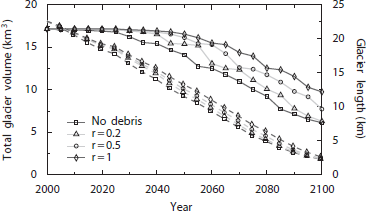
Fig. 9. Time evolution of the total ice volume (dashed curves) and of the glacier length (solid curves, right-hand-side axis) along the central flowline of Aletschgletscher for different parameters of the debris-evolution model according to scenario ENSmed.
When including the effect of supraglacial debris on the melting of bare ice, the glacier tongue can potentially survive for a long time, almost without any dynamics. The quasi-stagnation of the ice flow on the glacier tongue in the case of strong debris coverage is also evident from the simulated ice surface velocities that tend to zero. As our model does not take into account the expected thickening of debris, we may underestimate this effect. In the case of rapid debris propagation (r = 1) the entire glacier tongue of Grosser Aletschgletscher would be debris-covered by 2080 (Fig. 8). If the effect of supraglacial debris is neglected, it would have disintegrated almost completely by that time. Assuming slow debris propagation (r = 0.2), however, the shape of the glacier tongue differs only slightly from the no-debris case. Whereas debris coverage had only limited importance for the mass balance of Grosser Aletschgletscher over the past century, it was vital for Oberaletschgletscher. If debris coverage is not accounted for, the entire tongue would disappear by 2050 (Fig. 8). This is also evident in Figure 6: Oberaletschgletscher retreats even if glacier-friendly conditions prevail, as in 1978. If the effect of debris coverage is included in the simulation of this glacier, the retreat rate is significantly lower, even in the case of slow debris propagation (Fig. 8).
For all experiments, the difference in ice volume compared with the no-debris case is relatively small (Fig. 9). It increases to ∼2 km3 by 2030 for r = 1. The simulated ice volumes converged again towards 2100. The time evolution of the glacier length was affected significantly by the presence of a debris layer. When r = 1, simulated glacier length differed by up to 5 km compared to debris-free conditions (Fig. 9). The accelerated retreat of the terminus starts in 2025 if debris is not accounted for, but is delayed by more than two decades when debris is accounted for. The model results strongly depend on the choice of parameters that are difficult to constrain. For a slow propagation of the debris front, the effect is significant only over the first decades of the study period. The differences from the reference simulation, however, tend to increase in the case of fast debris propagation, as a significant part of the shrinking glacier surface area remains covered with debris (Fig. 8).
Conclusions
The past and future evolution of Grosser Aletschgletscher was simulated using a combined 3-D ice-flow and mass-balance model. Basal sliding was taken into account, resulting in an improved calculation of the velocity field. The evolution of the entire glacier cluster around Aletschgletscher and two nearby glaciers, was simulated from 1999 to 2100 using different climate scenarios based on RCMs of the ENSEMBLES project. In addition, an investigation was carried out into glacier response to an air-temperature increase referring to the political ‘two-degree target’, and steady climatic forcings of several selected periods in the past, extended over 100 years. The sensitivity of glacier retreat to the presence and possible future expansion of supraglacial debris was tested, based on a new model for spatio-temporal evolution of the debris cover.
For Grosser Aletschgletscher, there was a significant decrease in glacier ice volume and length by the end of the 21st century for most of the scenarios. According to the median RCM driven by the A1B emission scenario, the volume of Aletschgletscher will decrease by 90% by 2100 and the 15 km long glacier tongue will disintegrate completely. Assuming a linear 2°C increase in air temperature until 2100 leads to a retreat of the glacier tongue by ∼10 km. The strong imbalance of Grosser Aletschgletscher with the current climate conditions results in a 41% volume loss, if climate forcing is stabilized on the level of the last two decades. Cooler and wetter conditions, as in 1978, however, would cause the glacier to significantly advance over the maximum of its Little Ice Age extent in a time interval of 100 years. Taking into account the retarding effect of supraglacial debris on future glacier evolution indicates that this variable, which is often neglected in glacier modelling, can have a significant impact on the rate of glacier terminus retreat.
This study shows that future climate change in the Alps may lead to a dramatic retreat and an almost complete disintegration of the largest glacier in central Europe. Due to their long response times, the condition of large glaciers is presently far from balance, and these glaciers will most likely continue to retreat, even if overall air temperature does not increase further. Although the uncertainties in projections of future changes in meteorological variables given by RCMs are significant, our study indicates that Grosser Aletschgletscher will show a decrease in its current ice volume by 70% or more with each of the ENSEMBLES RCMs. Among the models considered in this paper, two have been considerably simplified. First, the basal sliding model does not account for the effects of subglacial meltwater and therefore cannot reproduce the increase in sliding due to an increase in runoff expected for a global warming scenario. Second, the incompletely understood feedback effects of glacier melt, such as the likely increase in supraglacial debris, have a strong impact on the reliability of glacier retreat modelling. We recommend that future research focuses on these processes, as it is important to include them in numerical models of glacier evolution.
Acknowledgements
G.J. is supported by the Swiss National Science Foundation, who funded this work through projects 200021-119721 and PBELP2-133349. We thank D. Farinotti and A. Bauder for providing bedrock topography and glacier surface elevation data. We are grateful to J. Rappaz and M. Picasso for support and to A. Caboussat and A. Masserey who provided the cfsMesh software that was indispensable for performing the simulations. MeteoSwiss is acknowledged for giving access to meteorological data, and Swisstopo for the glacier maps and aerial photographs. The delta change scenario data were distributed by the Center for Climate Systems Modeling (C2SM). The data were derived from regional climate simulations of the European Union sixth framework programme (FP6) integrated project ENSEMBLES (contract No. 505539). The dataset was prepared by T. Bosshard, partly funded by Swisselectric/Swiss Federal Office of Energy (BFE) and CCHydro/Swiss Federal Office for the Environment (BAFU). We thank Electra-Massa and the Canton of Valais for financial support, and S. Braun-Clarke for proofreading. Constructive comments by A. Vieli and an anonymous referee helped to improve the manuscript.
Appendix: A Debris-Evolution Model
We propose a simple model to describe the spatio-temporal evolution of supraglacial debris. Let Ω(t) and Γ(t) be the debris-covered area and its boundary at time t, and D(t, x, y) be the signed distance function to the interface, Γ(t), such that D(t, x, y) is positive in Ω(t) and negative elsewhere. By definition, the debris area boundary, Γ(t), is the zero level set of a function D = D(t, x, y). Level set functions are often used to describe a topologically changing domain (Reference Osher and FedkiwOsher and Fedkiw, 2003) (e.g. a set of debris). Fix t and assume Ω(t) is known, the signed distance is the stationary solution of
with initial condition ![]() , where
, where ![]() is positive in Ω(t) and negative elsewhere. The time evolution of debris is given by
is positive in Ω(t) and negative elsewhere. The time evolution of debris is given by
with initial condition D 0, which represents the initial debris area. In Equation (A2) C denotes the speed of the debris front in the outward normal direction. Both Equations (A1) and (A2) are nonlinear Hamilton–Jacobi equations, and are solved numerically using an upwind finite-difference scheme (Reference Osher and FedkiwOsher and Fedkiw, 2003).


