


1. Introduction
The motion of small plankton in the turbulent ocean is overdamped (Visser Reference Visser2011). Accelerations play no role, and hydrodynamic forces and torques can be computed in the Stokes approximation. Turbulence rotates these small organisms, yet they manage to navigate upwards towards the ocean surface. Gyrotactic organisms make use of gravity to achieve this. These bottom-heavy swimmers experience a gravity torque that tends to align against the direction of gravity, so that they swim upwards (Kessler Reference Kessler1985; Durham et al. Reference Durham, Climent, Barry, Lillo, Boffetta, Cencini and Stocker2013; Gustavsson et al. Reference Gustavsson, Berglund, Jonsson and Mehlig2016). Also density or shape asymmetries give rise to torques in the Stokes approximation that can change the swimming direction (Roberts Reference Roberts1970; Jonsson Reference Jonsson1989; Roberts & Deacon Reference Roberts and Deacon2002; Candelier & Mehlig Reference Candelier and Mehlig2016; Roy et al. Reference Roy, Hamati, Tierney, Koch and Voth2019).
Larger organisms accelerate the surrounding fluid as they move, and this changes the hydrodynamic force the swimmer experiences (Wang & Ardekani Reference Wang and Ardekani2012; Khair & Chisholm Reference Khair and Chisholm2014; Chisholm et al. Reference Chisholm, Legendre, Lauga and Khair2016; Redaelli et al. Reference Redaelli, Candelier, Mehaddi and Mehlig2022). Three different mechanisms cause such fluid-inertia effects: a non-zero slip velocity (Oseen problem with non-dimensional parameter  $Re_p$, the particle Reynolds number), velocity gradients of the disturbance flow (Saffman problem, shear Reynolds number $Re_s$) and unsteady fluid inertia (with parameter $Re_p\,Sl$, where $Sl$ is the Strouhal number).
Fluid inertia gives rise to hydrodynamic torques. For a passive spheroid in spatially inhomogeneous flow, there are  $Re_s$-corrections to Jeffery's torque (Subramanian & Koch Reference Subramanian and Koch2005; Einarsson et al. Reference Einarsson, Candelier, Lundell, Angilella and Mehlig2015; Rosén et al. Reference Rosén, Einarsson, Nordmark, Aidun, Lundell and Mehlig2015; Dabade, Marath & Subramanian Reference Dabade, Marath and Subramanian2016; Marath & Subramanian Reference Marath and Subramanian2018). A passive spheroid settling in a quiescent fluid experiences an inertial torque, a $Re_p$-effect. This Khayat-Cox torque tends to align the particle so that it settles with its broad side down (Brenner Reference Brenner1961; Cox Reference Cox1965; Khayat & Cox Reference Khayat and Cox1989; Klett Reference Klett1995; Dabade, Marath & Subramanian Reference Dabade, Marath and Subramanian2015; Kramel Reference Kramel2017; Lopez & Guazzelli Reference Lopez and Guazzelli2017; Menon et al. Reference Menon, Roy, Kramel, Voth and Koch2017; Gustavsson et al. Reference Gustavsson, Sheikh, Lopez, Naso, Pumir and Mehlig2019; Jiang et al. Reference Jiang, Zhao, Andersson, Gustavsson, Pumir and Mehlig2021; Cabrera et al. Reference Cabrera, Sheikh, Mehlig, Plihon, Bourgoin, Pumir and Naso2022). For a passive sphere, spherical symmetry ensures that the Khayat-Cox torque vanishes.
In this paper, we show that a small spherical squirmer experiences an inertial torque analogous to the Khayat & Cox torque when it settles in a quiescent fluid. Using asymptotic matching, we calculate the torque to leading order in the particle Reynolds number
 \begin{equation} Re_p = {au_{c}}/{\nu}, \end{equation}
where  $u_{c}$ is a velocity scale, $a$ is the radius of the squirmer and $\nu$ is the kinematic viscosity of the fluid. The calculation shows that the inertial torque does not vanish for a spherical swimmer because swimming breaks rotational symmetry. We describe how the torque aligns the squirmer, and compare its effect with gyrotactic torques, and with the Khayat-Cox torque for a non-spherical passive particle.
2. Model
We consider a steady spherical squirmer, an idealised model for a motile micro-organism developed by Lighthill (Reference Lighthill1952) and Blake (Reference Blake1971). In this model, one imposes an active axisymmetric tangential surface-velocity field of the form
 \begin{equation} (B_1 \sin\theta + B_2 \sin\theta\cos\theta)\hat{\boldsymbol{e}}_\theta, \end{equation}
with parameters  $B_1$ and $B_2$, and where $\theta$ is the angle between the swimming direction (unit vector $\boldsymbol {n}$) and the vector $\boldsymbol {r}$ from the particle centre to a point on its surface. The tangential unit vector at this point is denoted by $\hat {\boldsymbol {e}}_\theta$. One distinguishes two types of squirmers depending on the parameter $\beta = B_2/B_1$ (Lauga & Powers Reference Lauga and Powers2009): ‘pushers’ ( $\beta < 0$) and ‘pullers’ with $\beta > 0$. In the Stokes limit, a squirmer moving with velocity $\dot {\boldsymbol {x}}$ in a fluid at rest experiences the hydrodynamic force
 \begin{equation} {\boldsymbol{F}'}^{(0)} = 6 {\rm \pi}\varrho_f \nu a \left(\tfrac{2}{3}B_1 \boldsymbol{n}-\dot{\boldsymbol{x}} \right). \end{equation}
Here the superscript denotes the Stokes approximation, and  $\varrho _f$ is the mass density of the fluid. Following Candelier, Mehlig & Magnaudet (Reference Candelier, Mehlig and Magnaudet2019) and Candelier et al. (Reference Candelier, Mehaddi, Mehlig and Magnaudet2022), we use a prime to indicate that this is the hydrodynamic force on the squirmer, due to the disturbance it creates.
Plankton tends to be slightly heavier than the fluid. Therefore we allow the squirmer to settle subject to the buoyancy force
 \begin{equation} \boldsymbol{F}_g = \frac{4{\rm \pi}}{3}a^3 (\varrho_s-\varrho_f)\boldsymbol{g}, \end{equation}
where  $\varrho _s$ is the mass density of the squirmer, and $\boldsymbol {g}$ is the gravitational acceleration. In the overdamped limit, the steady centre-of-mass velocity of the squirmer is determined by the zero-force condition ${\boldsymbol {F}'}^{(0)} +\boldsymbol {F}_g=\boldsymbol {0}$. This yields $\dot {\boldsymbol {x}} = \frac {2}{3} B_1 \boldsymbol {n} + \frac {2}{9}({\varrho _s}/{\varrho _f}-1) ({a^2}/{\nu })\boldsymbol {g}\equiv \boldsymbol {v}_s^{(0)} + \boldsymbol {v}_g^{(0)}$. Again, the superscript denotes the Stokes limit. In this limit, the squirmer experiences no torque in a fluid at rest, ${\boldsymbol {T}^{\prime }}^{(0)} = \boldsymbol {0}$.
3. Inertial torque
Assume that the squirmer swims with swimming velocity  $\boldsymbol {v}_s$ and settles with settling velocity $\boldsymbol {v}_g$. The angle between $\boldsymbol {v}_s$ and $\boldsymbol {v}_g$ is denoted by $\alpha$, as shown in figure 1(a). Symmetry dictates the form of the inertial torque $\boldsymbol {T}^\prime$. It has the units mass $\times$ velocity $^2$. Since the torque is an axial vector, it must be proportional to the vector product between the two velocities. The torque can therefore be written as
 \begin{equation} {\boldsymbol{T}^\prime}^{(1)} = C m_f(\boldsymbol{v}_s \wedge \boldsymbol{v}_g), \end{equation}
where  $m_f = ({4{\rm \pi} }/{3})a^3 \varrho _f$ is the equivalent fluid mass, $C$ is a non-dimensional constant, and the superscript indicates that this is the first inertial correction to the torque. Equation (3.1) says that torque vanishes when the swimmer swims against gravity ( $\alpha = {\rm \pi}$ in figure 1a), and when it swims in the direction of gravity ( $\alpha =0$). Bifurcation theory implies that one of these fixed points is stable, the other one unstable. The sign of the coefficient $C$ determines which of the two is the stable fixed point.

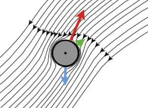
Figure 1. (a) Squirmer with swimming velocity  $\boldsymbol {v}_s$ and settling velocity $\boldsymbol {v}_g$, see § 2. Gravity points in the negative $\hat {\boldsymbol {e}}_2$-direction. (b,c) Disturbance flow created by a squirmer with $B_2=0$ (schematic). Shown are the flow lines in the frame that translates with the body. The centre-of-mass velocity $\dot {\boldsymbol {x}}$ is shown in green.
Inertial torques can be understood as a consequence of advection of fluid momentum. In the frame translating with the squirmer, far-field momentum is advected by the transverse disturbance flow generated by the squirmer, as illustrated schematically in figure 1(b,c). At non-zero  $Re_p$, the head of the squirmer – the north pole of the axial velocity field (2.1) – experiences more drag than its rear, because some of the momentum imparted to the fluid by the head is advected to the trailing end, in the direction transverse to gravity. So when $\boldsymbol {v}_s$ is not co-linear with $\boldsymbol {v}_g$ there is an inertial torque which rotates the swimmer so that $\boldsymbol {v}_s$ becomes closer to anti-parallel with $\boldsymbol {v}_g$. Comparing with (3.1), this means that the coefficient $C$ must be negative. Note that the mechanism described above is the same that creates Khayat-Cox torques on non-spherical passive particles sedimenting in quiescent fluid. For a fibre, for example, the far-field momentum is advected by the transverse flow along the fibre, leading to a torque that aligns the fibre perpendicular to gravity (Khayat & Cox Reference Khayat and Cox1989).
4. Perturbation theory for the coefficient  $C$
$C$

The inertial torque is computed from
 \begin{equation} {{\boldsymbol{T}}^\prime}^{(1)}= \int_{\mathscr{S}}\boldsymbol{r}\wedge(\mathbb \sigma^{(1)}\,\text{d}\boldsymbol{s}), \end{equation}
where  $\sigma _{mn}^{(1)} = -p^{(1)}\delta _{mn} + 2 \mu S_{mn}^{(1)}$ are the elements of the stress tensor $\mathbb \sigma ^{(1)}$ with pressure $p^{(1)}$, $S_{mn}^{(1)}$ are the elements of the strain-rate tensor of the disturbance flow and $\mu =\varrho _f \nu$ is the dynamic viscosity. The integral goes over the particle surface $\mathscr {S}$, $\boldsymbol {r}$ is the vector from the particle centre to a point on the particle surface and $\text {d}\boldsymbol {s}$ is the outward surface normal at this point. In the Stokes approximation the torque vanishes, ${{\boldsymbol {T}}^\prime }^{(0)}=\boldsymbol {0}$, as mentioned above.
The disturbance stress tensor is determined by solving the steady Navier–Stokes equations for the velocity  $\boldsymbol {w}$ of the incompressible disturbance flow caused by the squirmer,
 \begin{equation} -Re_{p} \dot{\boldsymbol{x}} \boldsymbol{\cdot} \boldsymbol{\nabla} \boldsymbol{w}+{Re}_{p} \boldsymbol{w} \boldsymbol{\cdot} \boldsymbol{\nabla} \boldsymbol{w} ={-} \boldsymbol{\nabla} p + \boldsymbol{\triangle} \boldsymbol{w}, \end{equation}
with boundary conditions  $\boldsymbol {w} = \dot {\boldsymbol {x}} + (B_1 \sin \theta + B_2 \sin \theta \cos \theta )\hat {\boldsymbol {e}}_\theta$ for $|\boldsymbol {r}|=1$, and $\boldsymbol {w} \to \boldsymbol {0}$ as $|\boldsymbol {r}|\to \infty$. Here we assumed that the squirmer has no angular velocity. We non-dimensionalised (4.2) using the radius $a$ of the squirmer as a length scale, and with the velocity scale $u_{c}=v_g^{(0)}$. Forces are non-dimensionalised by $\mu a u_{c}$, and torques by $\mu a^2 u_{c}$. The acceleration terms on the left-hand side of (4.2) are singular perturbations of the right-hand side, the Stokes part. We use matched asymptotic expansions in $Re_p$ to determine the solution for small $Re_p$ (Hinch Reference Hinch1995). Near the squirmer, one expands:
 \begin{equation} {\boldsymbol{w}}_{in} = {\boldsymbol{w}}_{in}^{(0)} + Re_p {\boldsymbol{w}}_{in}^{(1)} + \cdots \quad \mbox{and} \quad {p}_{in} = {p}_{in}^{(0)} + Re_p {p}_{in}^{(1)} + \cdots. \end{equation}
This inner expansion is matched, term by term, to an outer expansion:
 \begin{equation} \hat{{\boldsymbol{w}}}_{out} = \hat{\mathcal{T}}_{reg}^{\,\,(0)} + Re_p(\hat{\mathcal{T}}_{reg}^{\,\,(1)} + \hat{\mathcal{T}}_{sing}^{\,\,(1)} )+ \cdots. \end{equation}
Here  $\hat {\mathcal {T}}_{reg}^{\,\,(0,1)}$ are regular terms in the outer expansion, while $\hat {\mathcal {T}}_{sing}^{\,\,(1)}$ is singular in $\boldsymbol {k}$-space, proportional to $\delta (\boldsymbol {k})$ (Meibohm et al. Reference Meibohm, Candelier, Rosén, Einarsson, Lundell and Mehlig2016). The outer solution is obtained by replacing the boundary condition on the surface of the squirmer by a singular source term in (4.2), a Dirac $\delta$-function with amplitude $\boldsymbol {F}^{(0)} = -6{\rm \pi} (\frac {2}{3} B_1 \boldsymbol {n}-\dot {\boldsymbol {x}} )$. Since the non-linear term (quadratic in $\boldsymbol {w}$) is negligible far from the particle, the resulting equation can be solved by Fourier transform, yielding explicit expressions for $\hat {\mathcal {T}}_{reg}^{\,\,(0,1)}$ and $\hat {\mathcal {T}}_{sing}^{\,\,(1)}$ which serve as boundary conditions for the inner problems. The inner problem to order $Re_p^0$ is the homogeneous Stokes problem
 \begin{equation} {-} \boldsymbol{\nabla} {p}_{in}^{(0)} + \boldsymbol{\triangle} {\boldsymbol{w}}_{in}^{(0)} = \boldsymbol{0},\quad \boldsymbol{\nabla} \boldsymbol{\cdot} {\boldsymbol{w}}_{in}^{(0)}= \boldsymbol{0}, \end{equation}
with boundary conditions
 \begin{align} {\boldsymbol{w}}_{in}^{(0)} = \dot{\boldsymbol{x}} + (B_1 \sin\theta + B_2 \sin\theta\cos\theta) \hat{\boldsymbol{e}}_\theta \quad \mbox{for}\ {|\boldsymbol{r}|=1},\quad {\boldsymbol{w}}_{in}^{(0)} \sim \boldsymbol{\mathcal{T}}_{reg}^{\,\,(0)} \quad \mbox{as}\ |\boldsymbol{r}| \to \infty. \end{align}
This problem is solved in the standard fashion using Lamb's solution (Happel & Brenner Reference Happel and Brenner1965). The  $Re_p^1$-order inner problem is inhomogeneous:
 $$\begin{gather} -\boldsymbol{\nabla} {p}_{in}^{(1)} + \boldsymbol{\triangle} {\boldsymbol{w}}_{in}^{(1)} ={-} Re_p \dot{\boldsymbol{x}} \boldsymbol{\cdot} \boldsymbol{\nabla} {\boldsymbol{w}}_{in}^{(0)} + Re_p {\boldsymbol{w}}_{in}^{(0)}\boldsymbol{\cdot} \boldsymbol{\nabla} {\boldsymbol{w}}_{in}^{(0)},\quad \boldsymbol{\nabla} \boldsymbol{\cdot} {\boldsymbol{w}}_{in}^{(1)}= 0, \end{gather}$$
 $$\begin{gather}{\boldsymbol{w}}_{in}^{(1)} = \boldsymbol{0} \quad \mbox{for}\ {|\boldsymbol{r}|=1} \quad \mbox{and} \quad {\boldsymbol{w}}_{in}^{(1)} \sim \boldsymbol{\mathcal{T}}_{reg}^{\,\,(1)} +\boldsymbol{\mathcal{T}}_{sing}^{\,\,(1)} \quad \mbox{for}\ |\boldsymbol{r}|\to \infty. \end{gather}$$
To solve (4.6), we make the ansatz  ${\boldsymbol {w}}_{in}^{(1)} =(\boldsymbol {w}_{p} + \boldsymbol {\mathcal {T}}_{sing}^{\,\,(1)})+ \boldsymbol {w}_{h}$, where $\boldsymbol {w}_{p}$ is a particular solution and $\boldsymbol {w}_{h}$ is the homogeneous solution of (4.6a). For the pressure we write $p_{in}^{(1)} = p^{(1)}_{p}+p^{(1)}_{h}$. We first determine the particular solution $\boldsymbol {w}_{p}^{{(1)}}$ and $p^{(1)}_{p}$ by Fourier transform, as described in Candelier et al. (Reference Candelier, Mehaddi, Mehlig and Magnaudet2022). Then $\boldsymbol {w}_{h}^{{(1)}}$ and $p^{(1)}_{h}$ are determined using Lamb's solution. The boundary condition for $\boldsymbol {w}_{h}$ is $\boldsymbol {w}_{h}^{{(1)}}=- \boldsymbol {w}_{p}^{{(1)}}- \boldsymbol {\mathcal {T}}_{sing}^{\,\,(1)}$ on the particle surface. Having obtained ${\boldsymbol {w}}_{in}^{(1)}$, we compute the torque from (4.1). The torque comes from the particular solution of the first-order inner problem; there are no singular contributions at this order. Note also that for a passive spherical particle, spherical symmetry ensures that the particular solution does not contribute to the torque. Swimming breaks spherical symmetry, and this is the reason that torque does not vanish for a spherical squirmer. Given $p^{(1)}$ and $\boldsymbol {w}_{in}^{(1)}$, we can determine the inertial correction $\mathbb \sigma ^{(1)}$ to the stress tensor. Performing the integral in (4.1), we find the leading-order contribution to the torque,
 \begin{equation} {\boldsymbol{T}^\prime}^{(1)} ={-}\frac{3{\rm \pi}}{2} Re_p (\boldsymbol{v}_s^{(0)} \wedge \boldsymbol{v}_g^{(0)}). \end{equation}
In dimensional units, this corresponds to  ${\boldsymbol {T}^\prime }^{(1)} = -{\frac {9}{8}} m_f (\boldsymbol {v}_s^{(0)} \wedge \boldsymbol {v}_g^{(0)})$. The coefficient $C=-{\frac {9}{8}}$ is negative, as predicted by the argument summarised in § 3. So a spherical organism swimming downwards experiences a torque that tends to turn it upwards, causing the organism to swim against gravity.
5. Direct numerical simulations
We solved the three-dimensional Navier–Stokes equations for the incompressible flow using an immersed-boundary method (Peskin Reference Peskin2002). The interaction between squirmer and fluid was implemented by the direct-force method (Uhlmann Reference Uhlmann2005): to satisfy the boundary condition (2.1), the algorithm calculates the predicted fluid velocity on the surface of the squirmer. Based on the mismatch between the predicted velocity and (2.1), an appropriate immersed-boundary force is applied to the fluid phase to maintain the boundary conditions (2.1) on the surface of the squirmer. We used the improved algorithm of Kempe & Fröhlich (Reference Kempe and Fröhlich2012), Breugem (Reference Breugem2012) and Lambert et al. (Reference Lambert, Picano, Breugem and Brandt2013), because it is more precise for nearly neutrally buoyant particles. We used a cubic computational domain of side length  $L= 20a$ with periodic boundary conditions. The computational domain was discretised using a cubic mesh with resolution ${\rm \Delta} x$. The Navier–Stokes equations were integrated using a second-order Crank-Nicholson scheme (Kim, Baek & Sung Reference Kim, Baek and Sung2002) with time step ${\rm \Delta} t$, while the motion of the squirmer was integrated using a second-order Adams–Bashforth method. The numerical simulation of solid-body motion in a fluid is challenging at small Re $_p$. The mesh resolution ${\rm \Delta} x$ must be fine enough to resolve the shape of the body, so that the viscous stresses near its surface are accurately represented. In addition, the time step ${\rm \Delta} t$ must be small enough to resolve the viscous diffusion of the disturbance, ${\rm \Delta} t < {\rm \Delta} x^2/\nu$ (Appendix).
To determine the torque, we froze the orientation of the squirmer at a given angle  $\alpha$, but allowed the squirmer to translate. It was initially at rest. We measured the centre-of-mass velocity and the torque after the transient, when the disturbance flow was fully established. Figure 2(a) shows the numerical results for the inertial torque on a spherical squirmer for different values of $Re_p$, in comparison with the theory (4.7). The remaining parameter values used in the simulations are quoted in the caption for figure 2. We see that the simulation results approach the small- $Re_p$ theory as the particle Reynolds number decreases. For the smallest value of $Re_p$ we simulated, $Re_p=0.1$, the relative error is approximately 16 %. For $Re_p=1$, the difference is much larger, but the simulation results nevertheless agree qualitatively with the small- $Re_p$ theory. This is encouraging, because it allows us to draw qualitative conclusions about the effects of the torque on plankton (§ 6). We note, however, that the numerical results for $Re_p=1$ exhibit an asymmetry in their dependence on $\alpha$. Since the small- $Re_p$ theory yields a symmetric angular dependence of the torque, we attribute the asymmetry to higher-order $Re_p$-corrections.

Figure 2. (a) Non-dimensional inertial torque  ${\boldsymbol {T}^\prime }^{(1)}={T^\prime _3}^{(1)} \hat {\boldsymbol {e}}_3$ on a spherical squirmer. Shown is the theory, (4.7) (solid line), in comparison with direct numerical simulation results (§ 5) for different values of particle Reynolds number: $Re_p=0.1$ ( $\Box$), $Re_p=0.323$ ( $\Diamond$) and $Re_p=1$ ( $\circ$). The torque was non-dimensionalised by $\mu a^2 u_{c}$, where $u_{c}=v_g^{(0)}$. The angle $\alpha$ is defined in figure 1(a). Parameters: $B_1=1$, $B_2=0$, $v_s^{(0)}=2/3$, $v_g^{(0)}=1$. Mesh resolution $2a/{\rm \Delta} x = 36$, time step $\nu {\rm \Delta} t/{\rm \Delta} x^2 = 0.22$. (b) Non-dimensional torque for $\alpha =90$ as a function of $Re_p$; other parameters same as in (a). Also shown is (4.7). (c) Non-dimensional swimming speed ( $\diamond$) and settling speed ( $\Box$) from direct numerical simulations for $Re_p=0.323$; other parameters same as in (a). Also shown are the Stokes estimates $v_s^{(0)}$ (dashed) and $v_g^{(0)}$ (solid).
The small- $Re_p$ theory predicts that ${T_3^\prime}^{(1)}/Re_p$ approaches a $Re_p$-independent plateau as $Re_p\to 0$. Figure 2(b) indicates that this plateau is not yet reached for $Re_p=0.1$. We note that there is still a residual time-step dependence for $Re_p=0.1$. Decreasing the time step further from $\nu {\rm \Delta} t/{\rm \Delta} x^2=0.22$ to $0.11$ increases the numerical value by 2.4 %. The deviation between the small- $Re_p$ theory and the simulation result of 16 % at $Re_p=0.1$ is consistent with that of Jiang et al. (Reference Jiang, Zhao, Andersson, Gustavsson, Pumir and Mehlig2021), who numerically computed the Khayat-Cox torque for settling spheroids, and found that the simulation result is approximately 20 % lower at $Re_p\approx 0.3$ than the small- $Re_p$ theory. Kharrouba, Pierson & Magnaudet (Reference Kharrouba, Pierson and Magnaudet2021) found smaller differences for a slender cylinder settling in a quiescent fluid, between 8 % and 13 % for $Re_p=0.05$, depending on the orientation of the cylinder. Note, however, that they compared with the more precise slender-body theory ((6.13) in Khayat & Cox Reference Khayat and Cox1989). This approximation is more accurate as $Re_p$ grows than (6.22) in Khayat & Cox (Reference Khayat and Cox1989) which is the equivalent of (4.7) here.
Another indication that higher-order  $Re_p$-corrections are important comes from measuring settling and swimming speeds in the numerical simulations. We extracted the swimming speed using $\dot {\boldsymbol {x}} = v_s \boldsymbol {n} - v_g \hat {\boldsymbol {e}}_2$. Solving for $v_s$ gives $v_s = \dot {\boldsymbol {x}}\boldsymbol {\cdot } \hat {\boldsymbol {e}}_1/(\boldsymbol {n}\boldsymbol {\cdot } \hat {\boldsymbol {e}}_1)$. Figure 2(c) shows the measured swimming and settling speeds at $Re_p=0.323$. The settling speed is substantially smaller than the Stokes estimate, consistent with a significant $Re_p$-correction. The swimming speed is much closer to the Stokes estimate. This is because the data shown is for $\beta =0$, and the known $Re_p$-corrections to the swimming speed (Khair & Chisholm Reference Khair and Chisholm2014),
 \begin{equation} \boldsymbol{v}_s = \frac{2}{3} B_1 \boldsymbol{n}\left[1-\frac{3\beta}{20} Re_p + \left(\frac{\beta}{8}+\frac{11\,987}{470\,400}\beta^2\right) Re_p^2+\cdots\right], \end{equation}
vanish for  $\beta =0$. We note that the numerical results of Chisholm et al. (Reference Chisholm, Legendre, Lauga and Khair2016) indicate that $\boldsymbol {v}_s$ does not depend on Re $_p$ at all for $\beta =0$.
6. Conclusions
We showed that a spherical squirmer settling in a fluid at rest experiences an inertial torque, and computed the torque using matched asymptotic expansions. The calculation is similar to that of Cox (Reference Cox1965) for the inertial torque on a nearly spherical, passive particle settling in a quiescent fluid. This torque vanishes for a passive sphere, a consequence of spherical symmetry. A spherical swimmer experiences an inertial torque because swimming breaks this symmetry. The torque causes the squirmer to align with gravity so that it swims upwards. In other words, this torque acts just like Kessler's gyrotactic torque for bottom-heavy organisms.
For small plankton, the effect of the inertial torque is much smaller than the gyrotactic torque, at least for spherical shapes. We can see this by comparing the corresponding reorientation times. This time scale is defined as  $\tau _I = \frac {1}{2} (8{\rm \pi} \mu a^3)/T_{max}$, where $8{\rm \pi} \mu a^3$ is the rotational resistance coefficient for a sphere (Kim & Karrila Reference Kim and Karrila2013) and $T_{max}$ is the maximal magnitude of the torque. For the inertial torque, one obtains $\tau _I ={8} \nu /({3}v_s^{(0)} v_g^{(0)})$ (this and all following expressions are quoted in dimensional units). The reorientation time for the gyrotactic torque is $\tau _G = 3\varrho _s\nu /(\varrho _fgh)$ (Pedley & Kessler Reference Pedley and Kessler1987), where $h$ is the offset between the centre-of-mass and the geometrical centre of the squirmer, and $g = |\boldsymbol {g}|$. The ratio of these time scales is $\tau _I / \tau _G \sim gh/v_s^{(0)}v_g^{(0)}$, assuming $\varrho _s \approx \varrho _f$. Taking $h\sim 10^{-7}$ m (table 1 in Kessler Reference Kessler1986), we see that swimming and settling speeds need to be of the order of mm s $^{-1}$ for the reorientation times to be comparable. For small plankton, typical speeds tend to be much smaller (Kessler Reference Kessler1986).
For larger organisms, however, the inertial torque can be significant. With typical values for a copepod (Titelman & Kiørboe Reference Titelman and Kiørboe2003),  $v_s = 1$, $v_g = 0.2$ mm s $^{-1}$, as well as $\nu =10^{-6}$ m $^2$ s $^{-1}$, one finds an inertial reorientation time of the order of $\tau _I \sim 10$ s $^{-1}$. Kolmogorov times for ocean turbulence range from $\tau _{K}=\sqrt {\nu /\mathscr {E}}=100$ s for dissipation rate per unit mass $\mathscr {E}=10^{-6}$ cm $^2$ s $^{-3}$ to $\tau _{K}=1$ s for $\mathscr {E}=10^{-2}$ cm $^2$ s $^{-3}$. So the non-dimensional reorientation parameter $\varPsi =\tau _I/\tau _{K}$ (Durham et al. Reference Durham, Climent, Barry, Lillo, Boffetta, Cencini and Stocker2013) ranges from $0.1$ for weak turbulence to $10$ for strong turbulence. The Reynolds number is of order Re $_p \sim 1$ for speeds of the order of 1 mm, so that the $Re_p$-perturbation theory does not strictly apply. However, since the theory works qualitatively as we demonstrated above, we can nevertheless conclude that for weak turbulence, the inertial torque can have a significant effect on the angular dynamics of the organism.
Some motile micro-organisms are non-spherical (Berland, Maestrini & Grzebyk Reference Berland, Maestrini and Grzebyk1995; Faust & Gulledge Reference Faust and Gulledge2002; Smayda Reference Smayda2010). It has been suggested that a non-spherical settling squirmer experiences an inertial Khayat-Cox torque (Qiu et al. Reference Qiu, Cui, Climent and Zhao2022). Since the boundary conditions differ between passive and active particles, and since swimming breaks fore-aft symmetry, the inertial torque on a non-spherical squirmer may be different from the Khayat-Cox torque. However, we expect that the torque is still determined by the same physical mechanism, advection of fluid-momentum transverse to gravity. This may give rise to terms proportional to  $\sin (2\alpha )$, whereas the torque is proportional to $\sin (\alpha$) for the spherical squirmer. To make these speculations definite, one could compute the inertial torque for a nearly spherical squirmer in perturbation theory. A second open question is to determine the inertial torque for bottom-heavy, non-spherical organisms, the analogue of the inertial torque on passive particles with mass-density asymmetries (Roy et al. Reference Roy, Hamati, Tierney, Koch and Voth2019).
More generally, although the small- $Re_p$ perturbation theory may become quantitatively inaccurate for Reynolds numbers of order unity – where the torque begins to make a significant difference – the results tell us which non-dimensional parameters matter, and how to reason about the effect of boundary conditions, and the symmetries of the problem. The calculation illustrates the conceptual insight that the inertial torque comes from fluid motion transverse to the direction of gravity. Fluid momentum in this direction is advected along the swimmer by the transverse fluid velocity, resulting in a torque. In our case, the boundary conditions are different from those for passive particles, and so is the symmetry of the problem, because swimming breaks fore-aft symmetry. Nevertheless, the fundamental mechanism generating the torque is the same.

Figure 3. Convergence tests changing mesh resolution  ${\rm \Delta} x$ (a,c,e) and changing integration time step ${\rm \Delta} t$ (b,d,f). Settling speed of a passive sphere (a,b), compared with the numerical data of Dennis & Walker (Reference Dennis and Walker1971), extracted from figure 4 of Vesey & Goldenfeld (Reference Vesey II and Goldenfeld2007). Swimming speed of neutrally buoyant spherical squirmer with $\beta =0$, compared with (5.1), (Khair & Chisholm Reference Khair and Chisholm2014), (c,d). Panels (e,f) show the inertial torque.
Funding
B.M. was supported by Vetenskapsrådet (grant no. 2021-4452) and by the Knut-and-Alice Wallenberg Foundation (grant no. 2019.0079). L.Z. was supported by the National Natural Science Foundation of China (grant nos. 11911530141 and 91752205). This research was also supported in part by a collaboration grant from the joint China-Sweden mobility programme [National Natural Science Foundation of China (NSFC)-Swedish Foundation for International Cooperation in Research and Higher Education (STINT)], grant nos. 11911530141 (NSFC) and CH2018-7737 (STINT).
Declaration of interests
The authors report no conflict of interest.
Appendix. Details regarding the direct numerical simulations
This Appendix describes how we found the required mesh and time resolutions for our numerical simulations. We considered two test cases: a passive sphere settling under gravity, and a neutrally buoyant squirmer with  $\beta = 0$, $Re_p=0.1$ and $0.323$. To check convergence as the mesh resolution increases, we changed ${\rm \Delta} x/2a$, keeping $\nu {\rm \Delta} t/{\rm \Delta} x^2= 0.22$ constant. Settling and swimming speeds reached a plateau when we increased the mesh resolution (left column of figure 3). For $Re_p=0.323$, the settling speed varied by 1.1 % and the swimming speed varied by 1.3 % when we changed ${\rm \Delta} x/2a$ from 1/36 to 1/48.
We then checked for convergence as the step size  ${\rm \Delta} t$ was reduced, for fixed ${\rm \Delta} x/2a=1/36$. Again, both settling and swimming speeds reached plateaus as $\nu {\rm \Delta} t/{\rm \Delta} x^2$ decreased (right column of figure 3). For $Re_p=0.323$, when we halved $\nu {\rm \Delta} t/{\rm \Delta} x^2$ from $0.22$ to $0.11$, the settling and swimming speeds varied by 0.25 % and 0.79 %, respectively. Therefore, we used ${\rm \Delta} x/2a=1/36$ and ${\rm \Delta} t = 0.22{\rm \Delta} x^2/\nu$ for most of the numerical simulations discussed in the main text. At these parameter values, the simulated settling speed of a passively settling particle is approximately 1 % larger than the numerical calculation of Dennis & Walker (Reference Dennis and Walker1971), taken from figure 4 of Vesey & Goldenfeld (Reference Vesey II and Goldenfeld2007). The swimming speed of the squirmer is independent of $\textit{Re}_p$ in the range $[0.1,1]$, and it is 6.3 % larger than the theoretical value $v_s^{(0)} = 2B_1/3$. This error constrains the overall accuracy of the numerical method; it is slightly less accurate for the active compared with the passive particle.
Finally, consider the torque (bottom panels of figure 3). For  $Re_p=0.323$, the torque varied by approximately 1.5 % when we changed ${\rm \Delta} x/2a$ from 1/36 to 1/48 for $\nu {\rm \Delta} t/{\rm \Delta} x^2= 0.22$, and it varied by 1.6 % when we halved $\nu {\rm \Delta} t/{\rm \Delta} x^2$ from $0.22$ to $0.11$ for ${\rm \Delta} x/2a=1/36$.


 Open access