


Introduction
Students in primary school are susceptible to infectious diseases. The clustering activities of students and a lack of herd immunity to some diseases such as chickenpox and influenza have also placed students at high risk for infectious disease outbreaks. Compared with other age groups, primary school students are more likely to spread diseases to their families and peers during an outbreak [Reference Baer, Rodriguez and Duchin1–Reference Cheng, Channarith and Cowling3]. Early detection of infectious diseases among students enables swift responses to prevent secondary transmission and school-based outbreaks of these diseases. Syndromic surveillance is a system, which collect and analyse non-specific syndromes, such as daily hospital visits by symptomatic patients, specific out-of-counter drug sales in pharmacy, student absenteeism and frequency of internet searches on disease-related keywords [Reference Mandl4]. It has been reported to be an effective approach for early warning and responses to infectious disease outbreaks especially in primary schools. Absenteeism in primary schools represents a major and effective data source for many syndromic surveillance systems. Some studies have found that the school absenteeism reporting system could generate signals of mumps and influenza-like illness 2–4 days before the outbreak [Reference Fan5–Reference Crawford8].
However, several issues should be considered when using absenteeism data in syndromic surveillance systems. First, there is a tendency for daily counts of absenteeism to cluster at zero at school level, which is a phenomenon known as zero inflation (ZI) [Reference Moghimbeigi9, Reference Lambert10]. Previous study showed that even in schools of over 1000 students, the average daily absenteeism count was 0.37 [Reference Fan5]. This tendency occurs because most students are usually present at school, thus a zero value is recorded. Encountering the clustering at zero is common in surveillance systems, such as systems for rare disease or infectious disease outbreaks in specific areas or over specific time periods [Reference Lee11, Reference Malesios12]. The zero-valued data imply important information on diseases, such as morbidity and mortality of a specific disease and population awareness regarding the disease. Traditional methods are inappropriate for addressing the zero-valued data because these data violate the necessary assumption. For example, equality of the variance and the mean is assumed in the Poisson model, which is too restrictive for absenteeism data. This excess variability leads to so-called overdispersion. ZI can also contribute to the overdispersion [Reference Bandyopadhyay13]. Two models have been widely considered in the literature to deal with too many zero values and overdispersion [Reference Stroup14–Reference Rose16], i.e. the zero-inflated Poisson model (ZIP) and the zero-inflated negative binomial model (ZINB). Second, early warnings require daily or weekly data reporting which inevitably brings about repeated measurements. Repeated measurements taken over several time periods for each unit of study (i.e., primary schools or health units) are worthwhile, since they allow more precise parameter estimates and predictions. However, violations of the assumption of data being independent and identically distributed (I.I.D) is a huge challenge for standard regression methods. A distinctive feature of this type of longitudinal data is the exhibition of correlations. Moreover, this non-independence feature is more obvious within the same schools at the beginning of an outbreak. Several reports have indicated that introducing a random effect into each equation of the ZI model could account for the non-independence [Reference Min and Agresti17, Reference Monod18]. These ZIP model with random effects (ZIP-RE) and ZINB model with random effects (ZINB-RE) models can simultaneously account for ZI, overdispersion and non-independence [Reference Neelon, O'Malley and Normand19–Reference Huirong, Sheng and Stacia21].
This study used the ZIP-RE and ZINB-RE models to a syndromic surveillance dataset collected in a European commission-funded research project titled as ‘An Integrated Surveillance System for Infectious Disease in Rural China: Generating Evidence for Early Detection of Disease Epidemics in Resource-Poor Settings (ISSC)’ (No. 241900). The ISSC project was launched in Jiangxi and Hubei provinces in China in 2010 [Reference Yan22, Reference Yan23]. The objective of the ISSC study was to improve the early detection of infectious disease epidemics in rural China by integrating syndromic surveillance with case report surveillance systems. Three types of syndromic data were collected in the project: patients’ chief complaints, over-the-counter (OTC) medication (medicines sold directly to a consumer without a prescription from a healthcare professional) sales and school absenteeism. Although absenteeism in primary schools has been a major and effective data source in many syndromic surveillance systems, few articles have simultaneously accounted for the complexity of the absenteeism data structure, which is often clumped at zero, shows overdispersion and features non-independence, to improve the early detection of aberrations. Ignoring these features to issue early warnings is likely to produce biased and inefficient results [Reference Lee11, Reference Neelon, O'Malley and Normand19]. Therefore, the aims of this modelling study were to provide an appropriate zero-inflated random effects model to handle the absenteeism data using the surveillance data collected in the first implementation year of the ISSC, and subsequently, to evaluate and verify the validity and timeliness of this model-based method for early warnings of infectious disease outbreak or public health events with real cluster events happened during the second implementation year of the project.
Materials and methods
Description of data
The surveillance of school absenteeism was established from 1 October 2011 to 31 March 2014, in two rural counties of Jiangxi Province under the ISSC project, with the first 6 months (stage I) served as a pilot and the following 24 months (stage II) as the formal implementation. The ISSC system for school absenteeism was modified based on the findings and practicing experiences from the stage I pilot study in 16 selected primary schools. The formal implementation stage II was launched on 1 April 2012. With a 40% (15/38) coverage of the townships in the two study counties 62 of the 266 primary schools were enrolled, including 38 village schools, 15 township schools and nine county level schools. School absence was defined as a student missing classes for half a school day or more. The head teachers were responsible for reporting the daily number of absent students and the reasons for the absences into the central database of ISSC online. Other information for each absent student was also collected, including age, sex and class. After checking for logical errors and duplicated records, the raw data were backed up and were ready for automated analysis. For more details, please refer to the papers by Yan et al. [Reference Yan22, Reference Yan23].
Descriptions of models applied
The zero-inflated model is a mixture of a distribution (e.g., the Poisson or negative binomial distribution) and a point mass at zero. The ZI model has two components that correspond to two zero-generating processes: a binary process with a probability Θ and a Poisson (or negative binomial) process with a probability(1 − Θ). ZI models can be generically described as follows:
 $$\Pr (\Upsilon = y) = \left( \matrix{\Theta + (1 - \Theta )f\,(0),\matrix{ {} & {} & {{\rm if}\matrix{ {y = 0,} & {{\rm and}} \cr}} \cr} \hfill \cr (1 - \Theta )f\,(y),\matrix{ {} & {} & {\matrix{ {} & {\matrix{ {{\rm if}} & {y \gt 0,} \cr}} \cr}} \cr} \hfill} \right.$$
where $\Upsilon $ denotes the random variable corresponding to observations from a zero-inflated model and f(y) is the discrete probability distribution function of the Poisson or negative binomial (ZIP or ZINB) [Reference Huirong, Sheng and Stacia21]. The ZINB model is formulated similarly to the ZIP model except for the addition of a dispersion parameter (k), which can be explained by overdispersion to some extent. For both the ZIP and ZINB models, log it(Θ) and log (λ) are the link functions for the Bernoulli probability of occurrences and the mean of the Poisson/NB, respectively. Then, a pair of random effects (μ 1 and μ2) were introduced to the ZIP and ZINB to accommodate non-independence or correlation [Reference Huirong, Sheng and Stacia21, Reference Fang24]. This introduction sets up a zero-inflated model with random effects as follows:
 $$\log \left( {\displaystyle{\Theta \over {1 - \Theta}}} \right) = \log it(\Theta ) = W\gamma + \mu _1, $$
 $$\log (\lambda ) = {\rm X}\beta + \mu _2, $$
where W and X are vectors of covariates for the logistic and Poisson/NB components, respectively. γ and β are the corresponding vectors of the regression coefficients. μ 1 and μ 2 are the random intercepts in the Bernoulli and Poisson/NB parts of the model, respectively and are assumed to be uncorrelated (Cov(μ 12) = 0) and follow the bivariate normal distribution as below:
 $$\left[ {\matrix{ {\mu _1} \cr {\mu _2} \cr}} \right] \sim BVN\left( {\left[ {\matrix{ 0 \cr 0 \cr}} \right],\left[ {\matrix{ {{\rm Var}(\mu _1 )} & {{\rm Cov}(\mu _{12} )} \cr {{\rm Cov}(\mu _{12} )} & {{\rm Var}(\mu _2 )} \cr}} \right]} \right).$$
Procedures of modelling
As noted, statistical modelling of records of these data is challenged by the three features: clumping at zero, overdispersion and non-independence. To address the complexity of these data, the zero-inflated mixed effects model was applied through following four steps (Fig. 1):
Step 1: Building a ‘well-fitting’ model from the ZIP-RE and ZINB-RE models to address the three characteristics of the absenteeism data obtained from the first implementation year of the ISSC (1 April 2012 to 31 March 2013).
Step 2: Applying the resulting model to predict the ‘expected’ number of absenteeism events in the second implementation year (1 April 2013 to 31 March 2014).
Step 3: Computing the differences between the observations and the expected values (marked as O–E values) to generate an alternative series of data for early warning of disease outbreaks. To observe spikes of observations over expectations, the negative values were set to zero, and the following EARS-3C algorithms are based on a positive one-sided Cumulative Sum (CUSUM) calculation.
Step 4: Evaluating the early warning validity and timeliness of the two-data series (the raw observation data and model-based O–E values) via the EARS-3C algorithms with regard to the detection of real cluster events happened in the second implementation year.
Fig. 1. Flowchart of identifying and evaluating ZIP-RE model to detect abnormal in school absenteeism.
The ‘well-fitting’ model was determined based on both theoretical assumptions and the four criteria called as Akaike's information criterion (AIC), a corrected Akaike's information criterion (AICC), a Bayesian information criterion (BIC) and a log-likelihood test. Here the model with the lowest AIC or BIC value was considered to give the best fit. Since absenteeism was likely to be affected by a range of covariates, analysis of dummy variables were also introduced, including schooling month with January being the reference, county (A vs. B) and type of school (township, village schools vs. county schools). Both mixture equations of ZIP-RE and ZINB-RE assumed identical covariates, although this assumption is not absolutely necessary.
A ‘well-fitting’ model does not always mean a ‘meaningful’ model for application. In syndromic surveillance practices, a ‘meaningful’ aberration detection model is useful if it allows detection of the aberration and distinguishes a true outbreak signal from a large amount of data in a timely manner. Therefore, to demonstrate the performance of the early warning ability of the zero-inflated mixed effects model, we employed the Early Aberration Reporting System (EARS, http://www.bt.cdc.gov/surveillance/ears) [Reference Fang24–Reference Hagen26] to retrospectively compare the two-data series based on the real cluster events. All cluster events were detected and confirmed by the ISSC during the same period. The EARS system has three syndromic surveillance algorithms named as ‘C1’, ‘C2’ and ‘C3’, which require little or no prior data as a baseline. The baseline of C1 is the seven time points before the assessed time point. C2 is similar to C1 apart from a 2-day lag in the baseline definition. Both C1 and C2 can be considered Shewhart control charts and the thresholds are set at 3. C3 is quite different from the two other methods although it is based on C2. In C3, the expected value is based on the sum over three time points (the assessed time points and the two previous time points). The cumulative sum of the positive differences is similar to that of a CUSUM method. An alarm is raised if C3 exceeds 2.
All data analyses were performed using the NLMIXED procedure in the SASv9.3 (SAS Institute, Cary, North Carolina) and STATA (Version 14, StataCorp, College Station, Texas) software. EARS-3C was implemented using Microsoft Excel. All corresponding codes are available from the authors.
Results
General description of the absenteeism reporting
As described in the method, the data used here were obtained from the ISSC project from 62 primary schools in two counties of Jiangxi Province from 1 April 2012 to 31 March 2014. A total of 10 789 absenteeism events were reported in the first implementing year, and 11 347 were reported in the second year. The histograms of monthly absenteeism events during the first year were presented in Fig. 2, with the number indicated the percentage of zero values in each month. A similar data distribution were observed (not presented) in year 2. It was found that a remarkable ZI occurred varied from 49.2% to 66.8% and 54.9% in mean. More than half of the schools reported no absences every month. Apart from the large proportion of zeros, the distribution was slightly positively skewed, with most observations showing only one to three student absences, which most likely implies overdispersion.
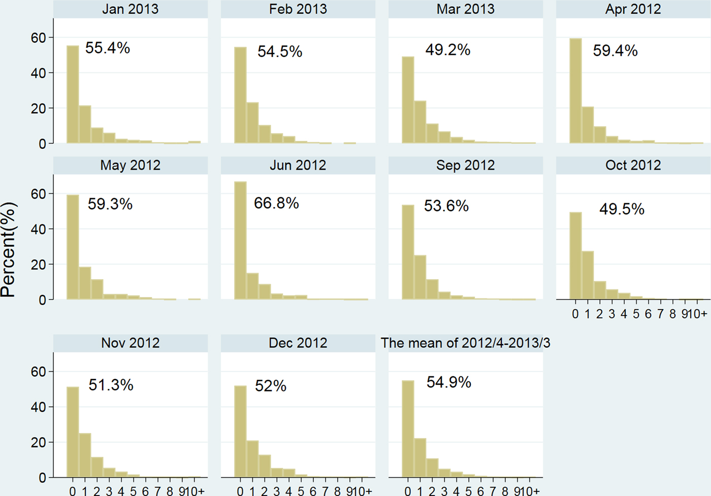
Fig. 2. Histogram of daily absence data from April 2012 to March 2013 Note: The percentages in the figure showed the level of zero% in each month.
The built of a ‘well-fitting’ model
The ‘well-fitting’ model was built using the ZIP-RE and ZINB-RE. The random effect component and information criteria for model selection were presented in Table 1. The details of modelling could be found in Appendix A. According to the information criteria, the ZIP-RE had a better fit than ZINB-RE because the AIC, AICC and BIC of ZIP-RE had much lower values. It was found that both of the two random effects of ZIP-RE (μ 1 and μ 2) were deviated from 0 with statistically significant differences (P < 0.05). The quantity of variance μ 1 (1.9617) was almost six times the quantity of variance μ 2. This finding suggested that there should be more variation in the probability of ‘whether absenteeism occurred or not’ than in the scale of ‘the seriousness of the absenteeism’. In brief, the modelling suggested that the ZIP-RE should be preferred to represent the characteristics of the zero-inflated and non-independent features in this study.
Table 1. Model selection results from ZIP-RE and ZINB-RE based on four information criteria and two random effects

Prediction, calculation of O–E values and assessment of the performance of the early warning system
After considering ZIP-RE as the ‘well-fitting’ model, the O–E values were further calculated. The EARS-3C algorithms were applied to retrospectively compare the early warning ability of the two-data series with regard to detecting the real cluster events. During the second implementation year, a total of 34 alarm signals were generated. Through a series of warning response processes, including data checking, preliminary judgement and epidemiologic investigation, a total of 18 ‘cluster’ or ‘outbreak’ events were confirmed. Of these ‘cluster’ events, seven were influenza, one was mumps, eight were chickenpox and two were due to heavy snow. To evaluate the early warning performance in detection these real cluster events, the raw observation values was compared with the O–E values.
The time trends and comparison between the two-data series were presented in Fig. 3 and the analysis details from the EARS-3C were summarised in Table 2. The two time series had similar trends of variation over time, and detected almost the same unusual signals corresponding to the real cluster events under the EARS-3C analysis. Therefore, a large part of Table 2 ‘agreed’, indicating that the two time series had equal performances.

Fig. 3. The time trends and key indicators of the observational data and O–E values analysed via EARS-3C Note: The topmost plot showed the time series of the raw observations of the numbers of absences (O) and the new index values (O–E). The red points indicated the starting dates of 18 cluster events. The EARS-3C results were shown in the bottom three plots (EARS-C1, EARS-C2 and EARS-C3). The red lines represented the thresholds for an alarm signal (3, 3 and 2). The open circles in the figure highlighted an inconsistency between the time series.
Table 2. Comparison of the early warning abilities between the observational data and the generated O–E values using the EARS-3C with regard to the real cluster events

Note: The first two columns are the identification dates of the 18 cluster events and their associated diseases. The following three columns are the results of comparisons using the EARS-3C algorithms. Inconsistencies are marked with shading. The last column is the inference to the validity and timeliness of O–E value series.
However, the performance of detecting cluster events of these two-data series showed some differences when different algorithms were applied. In the C1 algorithm, two cluster events were detected and generated alarm signals in the O–E index that were not detected using the raw absence data source (displayed as ‘alarm’). In another cluster event (the chickenpox outbreak on 12 November), the abnormal alarm-based O–E values were detected and generated 1 day in advance. In the C2 algorithm, all the signals were the same with the exception of one mumps epidemic that was successfully detected by the O–E values. C3 generated more inconsistent signals due to its higher sensitivity. The O–E values based on the ZIP-RE model method showed some advantages over the raw absence data source. Four abnormal clusters were detected ahead of time (displayed as ‘in advance’). Additionally, the raw data series but not the O–E values incorrectly generated three false-positive alarms (displayed as ‘false alarm’). However, a 1-day lagged detection of a chickenpox outbreak (20 November) in a primary school was found when using the O–E data source compared with using the raw data.
The inference was made based on above results presented in the last column (Table 2). The ZIP-RE-model index (O–E) had undoubtedly found all 18 cluster events using EARS-3C, whereas the raw data series failed to trigger either EARS-C1, C2 or C3 (see the first three rows in Table 2 marked as ‘detected’). Furthermore, the last three rows in Table 2 showed three false-positive alarms generated by the raw data series, which were not seen by the O–E values. Therefore, the ZIP-RE model could improve the early warning ability with high sensitivity and low false-positive errors. Meanwhile, the O–E index demonstrated better timeliness with four of the 18 cluster events detected in advance, although there was one delay in a chickenpox event on 20 November 2013.
Discussion
Unlike the infectious disease case reporting system with laboratory-confirmed diagnoses, the syndromic surveillance collects non-specific health information that constitute a ‘syndrome’, such as clinical chief complaints, symptoms and signs, and proxy indicators including school absenteeism, OTC drug sales in pharmacy, amount of online searching for disease related keywords, and changes of animal productivity [Reference Fearnley27, Reference Fouillet28]. Although a variety of data sources have been used for the early detection of infectious disease outbreaks and other public health events, school absenteeism is particularly useful because students are the most susceptible groups to the diseases. However, the absenteeism data have a tendency to contain a large proportion of zero observations. The absenteeism is a relatively infrequent event for a small primary school within a short time period except under exceptional conditions, such as an infectious disease outbreak, emergency incident or natural disaster. Moreover, zero records occur when daily monitor is required including weekends and holidays. Another possible source of excess zero is due to ‘mistakes’ [Reference Arab29], when the sick supposedly no-show students keep attendence because they would not like to miss the class. Thus, no absenteeism is observed and zero values appear. Consequently, any statistical method applied to this data should account for the excess zero values.
ZI models (e.g., ZIP/ZINB) offer an informative and elegant regression approach that allowed assessment of both the probability of zero and the severity of absenteeism in a specific school. Another widely used approach for the zero-inflated counts was the hurdle modelling (H) proposed by Mullahy [Reference Mullahy30] and Heilbron [Reference Heilbron31]. Although both of the two models (H and ZI) seem applicable for data with excess zero values, subtle differences exist. The H model includes a mass at zero and a truncated distribution, whereas the ZI model is based on an overlap of zero and a ‘regular’ distribution. Under this ZI model, the two sources of zeros are called ‘structural zeros’ and ‘sampling zeros’. The selection of the appropriate model depends on the study design, purpose and prior hypothesis about the distribution of the data. In this study, the zeros of absenteeism data had a tendency of the ‘mistake’ situations mentioned above. This scenario was typical of random ‘sampling zeros’, as argued by Arab [Reference Arab29]. Therefore, ZI model rather than H model were considered.
In addition, the hierarchical structure of the data (repeated observations within each school) implied that the observations are not independent, especially at the beginning of an infectious disease outbreak. Modelling repeated measures of zero-inflated count data is especially challenging. An alternative is to introduce random effects into a ZIP or ZINB model (named ZIP-RE and ZINB-RE, respectively). For this purpose, the ZIP-RE and ZINB-RE models were employed to fit the absenteeism data in our study. These zero-inflated mixed effects models have incorporated random effects into each component to account for ZI and longitudinal count measurements [Reference Neelon, O'Malley and Smith32, Reference Neelon, O'Malley and Smith33].The information criteria (AIC, BIC and AICC) corresponding to our data showed that the ZIP-RE model provided a significantly better fit than the other proposed models. Hence, we consider this model being a ‘well-fitting’ model.
Nevertheless, selecting a ‘good’ model cannot guarantee that the results would precisely reflect the real world. The study purpose and the questions to be answered must also be considered. Syndromic surveillance covers a wide range of purposes, especially for early warnings and detecting an anomalous, unexpected or emerging public health event (e.g., influenza or food-borne outbreaks) [Reference Fouillet28, Reference Triple34]. After building the ‘well-fitting’ model based on the first-implementation-year data, the real-world events happened in the second year were used to assess the early warning validity and timeliness of the two-data series (the raw observation data and model-based O–E values). It was found that the model-based O–E values detected three abnormal cases as presented in Table 2, whereas the original observation values did not detect any abnormal cases. In addition, when applying the EARS-3C algorithms, even both models could detect the four abnormal cases, the O–E values provided early warnings 1 or 2 days in advance. A previous simulation-based study had also found this issue to be a weak point of the current methods. Hutwagner et al. [Reference Hutwagner35] noted that the high sensitivity of the EARS-3C algorithms resulted in multiple false positives. However, in this study, the false-positive signals happened to the raw data were avoided via the new indicator of O–E values. Of course, this alternative method is not flawless. For instance, the new method delayed sending the warning signal for one of the chickenpox cases by 1 day.
It should be mentioned that there were limitations in this analytic study. First, the predicting analysis was based on 1-year historical data. Making predictions with short-term data incurs problems on uncertainty and fluctuations, and the secular trends in real world could be missed. Moreover, it was assumed that no infectious disease outbreaks occurred during the first implementing year. This situation was somehow impractical. Second, there are other possible causes of excessive zero values, such as weekends and holidays, which should also be considered in the model. Additionally, zero values only reflect the students’ situation at school. Integrating the absenteeism data with other data sources (e.g., outpatient visits, OTC medication sales) would be helpful towards early warning of disease outbreaks. Third, an early warning should not only focuses on ‘when did the outbreak occur’ but also ‘where was the cluster’. Therefore, considering spatial or spatiotemporal variability of absenteeism in primary schools is critical to a reliable assessment or prediction. Recently, studies in these fields have started to a Bayesian approach [Reference Malesios12, Reference Neelon, O'Malley and Normand19, Reference Jang, Lee and Kim36] or Integrated Nested Laplace Approximation with the considerations of spatial or spatiotemporal correlations [Reference Arab29, Reference Blangiardo and Cameletti37].
Conclusion
In summary, schools are ideal settings for the detection of aberrant cases, such as outbreaks of infectious diseases. After fully considering the characteristics of absenteeism data in primary schools, we conclude that ZIP-RE model using O–E values had the potential to improve the timeliness of early detection of aberrations, reduce the false-positive signals and eventually achieve the goal of detecting abnormal cases more quickly and accurately. With more applications, zero-inflated mixed effects model has considerable potentials to become a useful supplement to traditional methods.
Supplementary material
The supplementary material for this article can be found at https://doi.org/10.1017/S095026881800136X
Acknowledgements
We are grateful to Future Position X(FPX) for developing the web-based surveillance system. This project was led by Karolinska Institutet in Sweden and implemented together with Fudan University School of Public Health, Huazhong University of Science and Technology and the University of Heidelberg-Institute of Public Health (UKL-HD). Our thanks also go to the participating schools in the ISSC Project. In addition, we are grateful to the team members of the Jiangxi Provincial Centre for Disease Prevention and Control and the ISSC staff in the two counties (Fengxin and Youngxiu Centre for Disease Control and Prevention).
Financial support
The project is financially supported by a grant under the European Union 7th Framework Program (project no: 241900). The Fourth Round of Three-Year Public Health Action Plan of Shanghai, China (15GWZK0101), for discipline (Epidemiology) development in the School of Public Health, Fudan University had also provided support for the work of researchers and graduate students.
Conflict of interest
The authors have no conflicts of interest to declare.


