


Introduction
The dynamics of tidewater glaciers are governed by complex interactions between ice flow, the ocean and the atmosphere (Catania and others, Reference Catania, Stearns, Moon, Enderlin and Jackson2020). Changes in terminus position are often the dominant control on variations in tidewater-glacier surface velocity (Howat and others, Reference Howat, Joughin, Tulaczyk and Gogineni2005; Joughin and others, Reference Joughin2008a, Reference Joughin2012), but atmospheric forcing also influences tidewater-glacier dynamics, with seasonal variations in meltwater input to the ice-bed interface observed to drive spatially and temporally varying responses in glacier speed (Joughin and others, Reference Joughin2008b; Moon and others, Reference Moon2014; Kehrl and others, Reference Kehrl, Joughin, Shean, Floricioiu and Krieger2017). The influence of the hydrological system on the dynamics of fast-flowing tidewater glaciers, however, is poorly understood, with more observations necessary to constrain glacier behavior (Flowers, Reference Flowers2018).
One reason for the gap in knowledge is the low temporal resolution (weeks to months) of the satellite data that provide the majority of tidewater-glacier velocity observations (Moon and others, Reference Moon2014; Kehrl and others, Reference Kehrl, Joughin, Shean, Floricioiu and Krieger2017; Joughin and others, Reference Joughin, Smith and Howat2018). Short-term variations in ice flow in response to variations in meltwater have long been observed at alpine glaciers (e.g. Iken and Bindschadler, Reference Iken and Bindschadler1986) and, more recently, have been demonstrated for land-terminating and inland sectors of the Greenland Ice Sheet (e.g. Sole and others, Reference Sole2011; Bartholomew and others, Reference Bartholomew2012; Andrews and others, Reference Andrews2014). Tidewater glaciers tend to flow much faster than these previously studied regions, but few records with the high temporal resolution necessary to assess short-term variations in ice flow are available at tidewater outlets. Analysis of the available records is complicated by high background velocities and by the presence of multiple sources of short-timescale velocity variability. Tidewater-glacier flow in Greenland is affected by near-instantaneous velocity response to large calving events associated with glacial earthquakes (Amundson and others, Reference Amundson2008; Nettles and others, Reference Nettles2008; Murray and others, Reference Murray2015); by periodic flow modulation in response to tides (Lingle and others, Reference Lingle, Hughes and Kollmeyer1981; Echelmeyer and others, Reference Echelmeyer, Clarke and Harrison1991; Reeh and others, Reference Reeh, Mayer, Olesen, Christensen and Thomsen2000; de Juan and others, Reference de Juan2010; Podrasky and others, Reference Podrasky, Truffer, Lüthi and Fahnestock2014); and by multi-day flow variability in response to melt forcing (Andersen and others, Reference Andersen2010, Reference Andersen2011). An understanding of tidewater-glacier dynamics and hydrology acting on daily and finer timescales is required to discern hydromechanical drivers of ice flow and improve physics-based models for such glacier systems, which are responsible for much of Greenland's mass loss (Enderlin and others, Reference Enderlin2014; Mouginot and others, Reference Mouginot2019).
A spatially extensive, high-temporal-resolution timeseries of ice flow is available for Helheim Glacier, East Greenland (Nettles and others, Reference Nettles2008). The data have previously been used to demonstrate the sensitivity of the glacier to surface melt on multi-day timescales (Andersen and others, Reference Andersen2010, Reference Andersen2011), and to describe the glacier response to tidal forcing (de Juan and others, Reference de Juan2010) and large calving events (Nettles and others, Reference Nettles2008). In addition, Davis and others (Reference Davis, de Juan, Nettles, Elósegui and Andersen2014) demonstrated the presence of diurnal variations in flow not associated with ocean tidal forcing, using a single, near-terminus (<3 km), 21 d GPS record. Here, we investigate (1) spatial and temporal variability in diurnal flow across Helheim Glacier, from the terminus to 37 km up-glacier; and (2) a possible link to daytime melt forcing. We use Automatic Weather Station (AWS) data recorded on the glacier to evaluate whether and how melt magnitude and timing influence glacier velocity, and we consider physical mechanisms for surface-melt controls on diurnal velocity variations in this tidewater environment.
Data and methods
2.1 Stochastic-filter analysis of glacier surface positions
Networks of geodetic-quality, dual-frequency GPS receivers were deployed on Helheim Glacier, East Greenland, during the melt season from 5 July to 24 August in 2007 (DOY 186–234) and 30 June to 17 August in 2008 (DOY 182–230) (Fig. 1), providing a recording period of 21–54 d. The networks spanned an along-flow distance of 2–37 km from the calving front, with additional fixed stations at bedrock sites. GPS data were processed in kinematic mode using the TRACK module (Chen, Reference Chen1998) of the GAMIT/GLOBK software package (http://geoweb.mit.edu/gg/) to yield 15-s position estimates (Nettles and others, Reference Nettles2008; de Juan and others, Reference de Juan2010; Davis and others, Reference Davis, de Juan, Nettles, Elósegui and Andersen2014). We eliminate position estimates with unfixed biases. Typical formal uncertainties for the horizontal position estimates are 5–10 mm (Davis and others, Reference Davis, de Juan, Nettles, Elósegui and Andersen2014). We project the horizontal position time series onto a coordinate axis defined by the direction of the local mean horizontal velocity vector at each station to obtain position estimates in the along-flow direction (Fig. 2a). The mean velocity in the orthogonal (cross-flow) horizontal direction is zero.
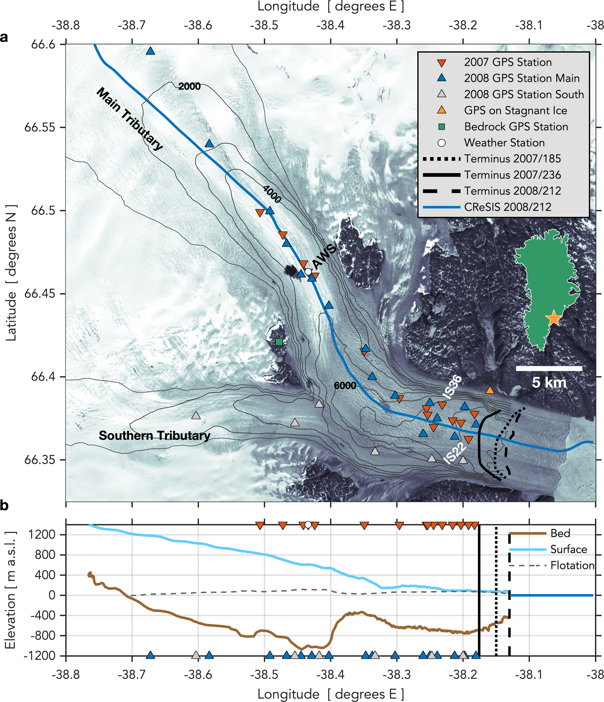
Fig. 1. Helheim Glacier, East Greenland. (a) Location of (triangles) GPS stations and (circle) Automatic Weather Station (AWS). Orange triangle shows station on stagnant ice. Calving-front position (black dotted, solid, and dashed lines) shown on 4 July 2007 (DOY 185), 24 August 2007 (DOY 236) and 30 July 2008 (DOY 212). July 2007 velocities from the MEaSUREs Greenland Ice Sheet Velocity Map (Joughin and others, Reference Joughin, Smith, Howat, Scambos and Moon2010; Reference Joughin, Smith, Howat and Scambos2015) shown in grey contours at 1000 m a−1 intervals, with the 2000, 4000 and 6000 m a−1 contours labeled. Background is Landsat image from 1 July 2001 (DOY 182) acquired from the United States Geological Survey (https://www.usgs.gov/). Inset shows (star) location of Helheim Glacier in Greenland. Blue line on panel (a) shows 30 July 2008 (DOY 212) Center for Remote Sensing of Ice Sheets (CReSIS) flight line for ice-sheet surface and bed elevations shown in panel (b) (CReSIS, 2020).

Fig. 2. Summary of stochastic-filter modeling approach for station IS22 horizontal positions from 5 to 25 July (DOY 186–206), 2007. (a) Along-flow station position; (b) detrended along-flow position x(t); (c) non-periodic along-flow speed v(t), relative to the IS22 mean speed of 22.4 m d−1; (d) ocean tidal admittance A(t); (e) lag in tidal response, τ(t); (f) estimated horizontal glacier response to ocean tide, A(t)F(t − τ(t)), from values shown in (d) and (e); (g) stochastic amplitude a c(t); (h) stochastic amplitude a s(t); (i) estimated horizontal diurnal variation in glacier position, x D(t), from values shown in (g) and (h); and (j) model residual ε(t). Station IS22 is located 2.3 km from the calving front (Fig. 1a). Grey shading shows ±1σ error bounds. Vertical grey lines show times of glacial earthquakes, which indicate major calving events. Data gaps resulting from elimination of noisy data are visible in the position (a) and residual (j) time series; the modeled values are continuous.
Following the methodology of Davis and others (Reference Davis, de Juan, Nettles, Elósegui and Andersen2014), we use a stochastic-filter approach (Chen, Reference Chen1998; Ravishanker and Dey, Reference Ravishanker and Dey2002; Davis and others, Reference Davis, Wernicke and Tamisiea2012) to model the time-dependent position of the glacier surface at each GPS site as the sum of three separate processes. The stochastic-filter approach is commonly used in geodesy and the analysis of geodetic observations of glacier flow; it is derived from standard least-squares methods, but the use of the stochastic-filter equations allows greater computational efficiency. Our approach is illustrated in Figure 2 for station IS22. The position estimates x(t), obtained every 15 s, are considered to result from (1) the time-integrated mean flow speed, $\mathop \int _{t_0}^t v( {t^{\prime}} ) {\rm d}t^{\prime}$ over the epoch t 0 to t; (2) a response to forcing by the ocean tides; and (3) a diurnal variation in position, x D(t). A contribution from noise in the position estimates, ε(t), is also allowed, such that the full model can be written

where x 0 = x(t 0) is the position at the initial epoch t 0, A(t) is the amplitude of the tidal admittance, F(t) is the tide height, and τ(t) represents a lag in the glacier response to the tide. All components on the right-hand side of Eqn (1) are estimated by the stochastic filter except for x 0. Following previous work, step changes in v(t) are allowed at the times of glacial earthquakes, which represent large calving events (Nettles and others, Reference Nettles2008; Davis and others, Reference Davis, de Juan, Nettles, Elósegui and Andersen2014).
Based on the results of de Juan and others (Reference de Juan2010) and Davis and others (Reference Davis, de Juan, Nettles, Elósegui and Andersen2014), we describe the response of the glacier position to the ocean tide using a linear admittance representation, A(t)F(t − τ(t)), where the amplitude of the tidal admittance A(t) is the ratio of the amplitude of the tidal response of the glacier to the amplitude of the ocean tide. The tide height F(t) is given by the AOTIM-5 model (Padman and Erofeeva, Reference Padman and Erofeeva2004), which was validated for this region using local observations (de Juan and others, Reference de Juan2010; Davis and others, Reference Davis, de Juan, Nettles, Elósegui and Andersen2014). When no tidal-modulation signal is present in the GPS position estimates, the estimates returned by the model for A(t) will be near zero. Preliminary analyses showed near-zero tidal-admittance values for stations more than ~10 km from the calving front, consistent with the results of de Juan and others (Reference de Juan2010); we therefore fix A(t) to zero at those stations.
The term representing a possible diurnal modulation of glacier position, x D(t), is written as

where f o is one cycle per day. For each amplitude a, the random-walk model is a(t + Δt) = a(t) + δa(t), where δa(t) is a Gaussian white-noise stochastic process with a mean of zero and a variance of σ2Δt. After testing variance rates σ2 ranging from 10−6 to 10−2 m2 d−1, we elect to use a value of 2 × 10⁻⁵ m2 d−1. The selected variance rate is the value above which the root-mean-square residuals begin to decline steeply, indicating the region of values for which the glacier positions would be overfit by the term of the filter representing possible diurnal modulation of glacier position. The time-varying amplitude of the diurnal signal, illustrated in Figure 3 for station IS22, is given by


Fig. 3. Stochastic-filter diurnal-position components and diurnal velocities for station IS22 from 5 to 25 July (DOY 186–206), 2007. (a) Diurnal positions x D(t) (equivalent to Fig. 2i), (b) diurnal-position amplitude $A_{x_{\rm D}}( t )$ , (c) diurnal velocities v D(t) and (d) diurnal-velocity amplitude $A_{v_{\rm D}}( t )$
 . Daily averages of diurnal-velocity amplitudes are shown with black diamonds in panel (d). Grey lines show ±1σ error bounds. Vertical grey lines show times of glacial earthquakes, which indicate major calving events.
We obtain the diurnal velocity signal v D(t) by differentiating x D(t), but neglect the small terms associated with the rate of variation of the stochastic amplitudes a s(t) and a c(t), such that

The time-varying amplitude of v D(t) is then

The diurnal position amplitudes $A_{x_{\rm D}}$ have std dev. of ~0.005 m, calculated by propagating the errors in a s(t) and a c(t) through Eqn (3) using the filter-determined std dev. in a s(t) and a c(t), and we consider x D(t) to be unresolved below this level. The corresponding resolution amplitude for the diurnal velocity v D(t) is 0.005(2πf o) = 0.03 m d−1, and we consider v D(t) to be unresolved below this level.
We illustrate the modeling approach for station IS22, which operated in 2007 at a location 2.3 km from the calving front, in Figures 2 and 3. Results from this station are representative of the lower terminus region, and a similar analysis was presented by Davis and others (Reference Davis, de Juan, Nettles, Elósegui and Andersen2014). In Figure 2, panel (a) shows the along-flow component of station position. This site moves more than 400 m during days 186–206. Panel (b) shows the detrended position, where the trend removed represents the average glacier speed at this site during the observing period (the trend seen in panel (a)). Panel (c) shows v(t) estimated from Eqn (1), where the speed is given with respect to the mean speed of 22.4 m d−1. Step changes in speed associated with glacial earthquakes occur near the start of day 190. Because this station is located near the glacier terminus, the data show a tidal modulation of flow. The estimated time-varying admittance and lag parameters, A(t) and τ(t) are shown in panels (d) and (e), respectively. Shown in panel (f) is the tidally modulated component of flow, A(t)F(t − τ(t)). This station also shows diurnally modulated flow; the time-varying diurnal parameters a c(t) and a s(t) are shown in panels (g) and (h), respectively. The full diurnal position signal x D(t) (Eqn (2)) is shown in panel (i). Finally, the time-varying residual, ε(t), is shown in panel (j). Gaps in the data visible in panels (a) and (j) arise from the elimination of noisy data (i.e. those data with biases unfixed in the TRACK position estimates). Short-duration (<4 h), low-amplitude excursions in the v(t), A(t), a c(t) and a s(t) parameters (e.g. excursions observed on DOY 197–200; Figs 2c, d, g, h) are likely the result of multipathing and/or ionospheric disturbances (Sohn and others, Reference Sohn, Park, Davis, Nettles and Elosegui2020). The modeling approach successfully separates the periodic variability in the glacier flow into a primarily semidiurnal tidal component and a diurnal component, such that neither the velocity term v(t) nor the residual ε(t) show remaining periodicity.
The derivation of diurnal velocities and diurnal-velocity amplitudes for station IS22 is shown in Figure 3. The estimated stochastic amplitudes a c(t) and a s(t) (Figs 2g, h) are used to construct the time-varying diurnal-position amplitude $A_{x_{\rm D}}( t )$ (Fig. 3b), calculated as in Eqn (3). Panel (c) shows the diurnal velocity, v D(t), calculated from Eqn (4); and panel (d) shows the time-varying amplitude of the diurnal velocity, $A_{v_{\rm D}}( t )$
 , calculated as in Eqn (5). Panel (d) also shows the daily-average values of diurnal-velocity amplitude for this station; these are the values used in our melt-sensitivity analysis (see Section 3 ‘Results’).
2.2 Resistive stress associated with diurnal speed variations
We apply a simplified force-balance technique to estimate the magnitude of resistive stresses associated with diurnal speed variations. Assuming that bed tractions balance driving stresses allows for a rough estimation of the decrease in traction that would be consistent with observed diurnal velocity changes. Following Joughin and others (Reference Joughin2012), we calculate the enhanced driving stress, τe, which is the sum of the gravitational driving stress τd and the longitudinal frontal stress τF (Howat and others, Reference Howat, Joughin, Tulaczyk and Gogineni2005; Cuffey and Paterson, Reference Cuffey and Paterson2010; Joughin and others, Reference Joughin2012). The longitudinal frontal stress τF arises from the presence of a free calving face (Howat and others, Reference Howat, Joughin, Tulaczyk and Gogineni2005; Joughin and others, Reference Joughin2012). The region of the terminus over which this stress is distributed depends on the stress-coupling distance (Kamb and Echelmeyer, Reference Kamb and Echelmeyer1986). Given the significant rise in bed topography and surface slope at ~12 km inland from the Helheim terminus (Fig. 1a), we assume τF influences the enhanced driving stress up to 12 km from the terminus (15 ice thicknesses) (Howat and others, Reference Howat, Joughin, Tulaczyk and Gogineni2005), approximately the same region over which the tides are observed to modulate glacier flow (de Juan and others, Reference de Juan2010). For our Helheim Glacier flowline geometry, we calculate a maximum τF value of 40 kPa at the terminus. Following Joughin and others (Reference Joughin2012), we assume τF decreases linearly from 40 kPa at the terminus to zero at a distance of 12 km inland. Driving stresses τd at the locations of the GPS stations range from 150 to 900 kPa, and are estimated from BedMachine3 ice-sheet surface and bed elevations (Morlighem and others, Reference Morlighem2017).
We then assume velocity is proportional to the enhanced driving stress raised to some power: $V\sim {\rm \tau }_{\rm e}^m$ , where m is a sliding exponent, with m = 3 for hard-bedded sliding (Weertman, Reference Weertman1957) and m → ∞ for soft-bedded sliding (Tulaczyk and others, Reference Tulaczyk, Kamb and Engelhardt2000; Cuffey and Paterson, Reference Cuffey and Paterson2010; Joughin and others, Reference Joughin, Smith and Schoof2019). To estimate the change in resistance required to explain diurnal variations in surface velocities, we estimate the average change in the enhanced driving stress, Δτe, needed to modulate speeds around the mean along-flow speed for each station following ${{\Delta v_{\rm D}} \over V} = \left[{{{\Delta {\rm \tau }_{\rm e}} \over {{\rm \tau }_{\rm e}}}} \right]^m$
 , where Δv D is the average amplitude of diurnal velocity variations over the time series and V is the average velocity, defined as the total along-flow position change (e.g. Fig. 2a) divided by the total duration of the time series.
2.3 AWS data and surface melt rate
An AWS collected hourly meteorological measurements during the second half of the 2007 observation season (27 July–23 August (DOY 208–233)) and all of the 2008 season (30 June–19 August in 2008 (DOY 182–232)). The AWS was installed in approximately the same location (66.46° N, 38.44° W) at the start of the AWS observation periods in 2007 and 2008 (Fig. 1a) (Andersen and others, Reference Andersen2010). The station recorded a standard suite of meteorological parameters, including incoming and reflected short-wave radiative fluxes (Fig. 4), and, in 2008, surface ablation (Andersen and others, Reference Andersen2010). The net short-wave radiative flux Q SW (insolation) closely correlates with the total energy flux available for melting, based on a surface-energy-balance model (Andersen and others, Reference Andersen2010).

Fig. 4. Automatic Weather Station (AWS) measurements and local melt. (a) AWS observations of daily integrated net shortwave radiation Q SW (insolation) and daily sonic-ranger ablation rate for 30 June–19 August (DOY 182–232) in 2008. Red line shows linear fit. (b) Integrated Q SW versus ablation in 2008. Red line shows linear fit. (c) (blue, left axis) Q SW and (red, right axis) ablation rate for a subset of the 2008 AWS observations, where ablation rate is calculated after smoothing ablation-ranger measurements with a 6 h moving-average filter. (d) Time of peak Q SW and peak ablation rate over the entire 2008 AWS observation record, where time of peak is the maximum value in the record after smoothing measurements with a 6 h moving-average filter. Horizontal lines and shading show mean time of peak for (blue) Q SW and (red) ablation rate ±1 std dev.
We observe a significant linear relationship between daily integrated Q SW and daily surface ablation (Fig. 4a), a strong linear relationship between surface ablation and time-integrated Q SW (Fig. 4b), and a temporal relationship between hourly observations of Q SW and ablation rate (Fig. 4c). Together, these relationships between surface ablation and Q SW allow us to use Q SW as a reasonable proxy for melt rate throughout the full time period of AWS observations in this study. This proxy allows us to investigate the relationship between diurnal velocities and melt rate in the 2007 observation season, when surface ablation observations were not taken. While surface ablation observations over a range of elevations would be preferable, data from only one AWS are available, and they are especially valuable because they were made on the glacier surface. On an annual timescale, cumulative melt-season surface runoff over the Helheim Glacier catchment is estimated to be 1.3 ± 0.2 km3 a−1 in 2007 and 1.0 ± 0.2 km3 a−1 in 2008, compared to a mean estimate of 1.0 ± 0.2 km3 a−1 for the period 1999–2008 (Mernild and others, Reference Mernild2010).
Results
Our stochastic-filter approach partitions observed glacier motion into a background-velocity term (Fig. 2c); a tidal-modulation term (Fig. 2f); and a non-tidal diurnal-modulation term (Fig. 2i). Our background-velocity and tidal-modulation results are consistent with those of previous studies (Nettles and others, Reference Nettles2008; de Juan and others, Reference de Juan2010; Davis and others, Reference Davis, de Juan, Nettles, Elósegui and Andersen2014; Voytenko and others, Reference Voytenko2015). Similar to Nettles and others (Reference Nettles2008), we find that along-flow motion over the array is dominated by mean flow speeds ranging from 23 m d−1 near the terminus to 4 m d−1 at 37 km up-glacier. Along-flow velocities across the network vary by 0.5–3 m d−1 around the mean values and show characteristic step-change increases at the times of large calving events, associated with glacial earthquakes (Fig. 2c). Stations <10 km from the terminus exhibit variations in flow due to the ocean tide (Fig. 2f), which is principally semidiurnal at this location, in agreement with the findings of de Juan and others (Reference de Juan2010). At these stations, tidal admittances A of ~−0.03 and lags τ of ~1–2.5 h are typical (Figs 2d, e). The variation in position attributable to the tide (Fig. 2f) is thus ±0.05 m for peak tidal amplitudes of ±1.5 m, with the position of the glacier most advanced 1–2.5 h after low tide, again consistent with previous results (de Juan and others, Reference de Juan2010; Davis and others, Reference Davis, de Juan, Nettles, Elósegui and Andersen2014; Voytenko and others, Reference Voytenko2015). Farther up-glacier, the tidal amplitude and lag cannot be resolved, and we fix the admittance term to zero at those stations. The stochastic residuals ε(t) lack obvious coherent time-varying signals (Fig. 2j). The root-mean-square residuals for the individual timeseries (Fig. 2j) are on the order of 10 mm.
All stations exhibit diurnal speed variations v D(t) (Fig. 5a) above the 1-σ uncertainty amplitude of ~0.03 m d−1 for all or portions of the observing period in both 2007 and 2008 (Figs 6a, d), with the exception of one station on stagnant ice isolated from the main glacier flow (Fig. 1a; this station is not shown in Fig. 6). Stations within 5 km of the terminus exhibit diurnal speed variations ten times larger than the 1-σ uncertainty amplitude, or ~±0.3 m d−1 (Fig. 5a). The amplitude of the diurnal velocity variation decreases away from the terminus, with similar behavior seen on the main trunk of Helheim Glacier and on the southern tributary (Fig. 7a). We observe variations in the amplitude of the diurnal velocities on multi-day timescales, with those variations being generally consistent across the network (Figs 6a, d). Across all stations, the average time of peak diurnal velocity occurs at 21.0 ± 0.3 h UTC in 2007 and 21.0 ± 0.6 h UTC in 2008 (Figs 6c, f), with the time of the peak best defined at stations where the diurnal speed amplitudes are largest. (The uncertainties given represent one std dev. in the average time across all stations.) We observe no spatial gradient in the time of peak diurnal velocity with distance along the glacier flowline in either 2007 or 2008 (Figs 6c, f, 7b).

Fig. 5. Diurnal variations in glacier surface speed at station IS36 and insolation at the AWS from 28 July to 22 August (DOY 209–234), 2007. (a) Diurnal speed, v D(t); blue shading shows ±1σ uncertainty. (b) AWS hourly observations of insolation, Q SW. (c) IS36 diurnal speed, v D(t), and hourly observations of insolation, Q SW, from panels (a) and (b), where the symbol color indicates hour of day (UTC). Arrow shows direction of increasing time.

Fig. 6. 2007 and 2008 diurnal-velocity amplitude and time of peak. (a) (diamonds) Daily average diurnal-velocity amplitude from 5 July to 24 August (DOY 186–234) in 2007, where color indicates station distance from the terminus. The grey shaded region at the bottom of the plot marks where v D(t) amplitudes are below 0.03 m d−1, the approximate limit of diurnal velocity resolution given GPS data quality (see Methods). (b) Integrated daily insolation. (c) (diamonds) Time of peak v D(t) and (circles) time of peak insolation Q SW in 2007. Red horizontal line shows average time of peak diurnal velocity across all stations ±1 std dev. around the average (red shaded region). Panels (d, e, and f) show equivalent values for 2008 observations from 30 June to 17 August (DOY 182–230). Vertical grey lines show times of glacial earthquakes, which indicate major calving events.

Fig. 7. Diurnal velocity average amplitude, temporal lag and sensitivity to insolation. (a) Average amplitude of v D(t) over observation period. Error bars show ±2 std dev. around the average. Solid lines show weighted exponential regression to data. (b) Time lag between time of peak v D(t) and time of peak insolation Q SW over observation period. Error bars show ±2 std dev. around the average. (c) Sensitivity, s, of diurnal velocities to daily integrated insolation for (red) 2007, (blue) 2008 main tributary and (grey) 2008 southern tributary. Error bars show ±2σ uncertainty in s. Solid lines show weighted exponential regression for (red) 2007 and (blue) 2008 main tributary.
AWS-observed insolation Q SW varies diurnally (Fig. 5b). Insolation values are nearly zero during the first 6 h of the day and increase to peak insolation at ~14.5 h UTC (Fig. 5c) (local time is UTC−2 h). We observe a highly consistent time of peak insolation for days when total daily integrated insolation is above 10 MJ m−2, with variations generally occurring on days when integrated insolation is <10 MJ m−2 (Figs 6b, c, e, f). Peak diurnal velocities lag peak insolation at the AWS station at all stations on nearly all days of observation (Figs 6c, f), with exceptions on 8 intermittent days in 2008 (DOY 183, 195, 196, 199, 209, 211, 215 and 216) at stations where the diurnal velocity is small in amplitude (Fig. 6f). With the exception of the station furthest away from the terminus in 2008, where the diurnal velocity is small in amplitude, we observe no difference along the glacier flowline in the lag between time of peak insolation and time of peak diurnal velocity (Fig. 7b). The average lag across all stations and both years is 6.5 ± 0.5 h.
Despite the relatively small range of total daily insolation values observed during our ~2-month time series, taken during a slowly varying part of the yearly insolation cycle, and the relatively small range of diurnal amplitudes observed at individual stations, we observe a positive relationship between total, daily integrated insolation and diurnal velocity amplitude at the stations with the best-resolved diurnal velocities (Fig. 8). We take the slope of the linear regression between daily integrated insolation and diurnal velocity amplitude to describe the sensitivity of the diurnal velocity to the magnitude of insolation. The sensitivity of this velocity amplitude to insolation is largest near the terminus, decreasing up-glacier (Fig. 7c). We do not interpret the intercepts of the linear regression between diurnal velocity amplitude and daily integrated insolation, keeping in mind that the latter is only a proxy for melt.

Fig. 8. Relationship between daily integrated insolation at the AWS and average daily v D(t) amplitude for a selection of GPS stations in 2007 and 2008. Color of the observation indicates the day of year in (a–f) 2007 and (g–l) 2008. Slope of linear regression, s, describes the sensitivity of the diurnal velocity to the magnitude of insolation, and is given with ±1σ uncertainty. Dashed lines show 95% confidence interval for linear regression. Coefficient of correlation, R, and p-value of the linear regression are given. Examples are typical of stations showing (a–c, g–h) better-constrained sensitivity values, and those (e–f, i, l) with small diurnal amplitudes where the relationship cannot be resolved.
Discussion
4.1 Diurnal speed variations
We observe diurnal velocity variations to occur across the lower ~37 km of Helheim Glacier over 96 melt-season days from 5 July to 24 August in 2007 (DOY 186–234) and 30 June to 17 August in 2008 (DOY 182–230) (Fig. 7a), with peak velocities lagging peak diurnal melt at the AWS (Fig. 7b). A simple interpretation is that the diurnal velocity variations result from melt reaching the ice-bed interface and reducing resistance to sliding. Because the speed-up is coherent along the glacier and lacks a discernible gradient in time of peak diurnal velocity (Fig. 7b), the variations are unlikely to result from tidal forcing or from marginal processes such as a diurnal weakening of the proglacial ice mélange. Changes in proglacial ice mélange are linked to variations in terminus position and velocity variations for Greenland tidewater glaciers on seasonal and interannual timescales (Moon and others, Reference Moon, Joughin and Smith2015; Kehrl and others, Reference Kehrl, Joughin, Shean, Floricioiu and Krieger2017; Bevan and others, Reference Bevan, Luckman, Benn, Cowton and Todd2019), but ice-mélange rigidity in Sermilik Fjord has not been observed to vary on diurnal timescales, in contrast to the persistent diurnal velocity variations we observe.
The 6.5 h lag between peak melt production and peak velocity shows low interstation variability (Figs 6c, f) and no spatial gradient along the flowline (Fig. 7b). This result is consistent with observations of supraglacial hydrology at Helheim, where there is little surface transport of meltwater and surface melt drains into local crevasses (Andersen and others, Reference Andersen2011; Everett and others, Reference Everett2016). Satellite imagery over our study area shows extensive crevassing and little evidence of surface transport of meltwater (Fig. 1a). The lag between melt production and diurnal velocities at Helheim is also consistent with the wide range of meltwater surface-to-bed transport times observed in land-terminating sectors of the Greenland Ice Sheet (Smith and others, Reference Smith2017). In land-terminating sectors, peak diurnal velocities are in phase with peak moulin hydraulic head (Andrews and others, Reference Andrews2014) or peak supraglacial stream discharge (Smith and others, Reference Smith2017). Stream discharge peaks 0.5–9.5 h after peak runoff production, with longer delays associated with larger areal extents of supraglacial catchments (Smith and others, Reference Smith2017). Because most crevasses at Helheim lack a direct connection to the bed, we interpret the delay between melt production and peak diurnal velocity to be due to the time needed for the water to transit through the englacial hydrologic system (Colgan and others, Reference Colgan2012). This interpretation for Helheim Glacier differs from the land-terminating regions where transit of melt across the ice-sheet surface leads to the lag between peak runoff production and diurnal velocities, and suggests the need for additional observational and theoretical work.
Recent observations of bulk englacial meltwater variability at Helheim Glacier (Vaňková and others, Reference Vaňková, Voytenko, Nicholls, Parizek and Holland2018) share similar diurnal fluctuation characteristics with the diurnal velocity variations we observe (Fig. 9), although the measurements are from different melt seasons: our data are from 2007 and 2008 whereas the Vaňková et al. dataset is from August 2015. Vaňková and others (Reference Vaňková, Voytenko, Nicholls, Parizek and Holland2018) find that englacial meltwater content peaks daily at ~14–16 UTC (Fig. S3 in Vaňková and others, Reference Vaňková, Voytenko, Nicholls, Parizek and Holland2018), similar to the time of peak insolation recorded by our AWS (Fig. 9). This englacial meltwater content likely reflects basal water pressure in some way, whether that be a direct representation of basal water pressure as observed in moulin hydraulic head (e.g. Andrews and others, Reference Andrews2014) or as a proxy for meltwater movement from the englacial to the basal drainage system. Taking the rate of change of englacial meltwater content as a proxy for water flux to the basal drainage system suggests peak meltwater flux to the bed occurs at ~20.5 h UTC (Fig. 9). The diurnal velocity variations we observe closely track meltwater flux into the basal system, with peak velocities observed at 21.0 ± 0.3 h UTC in 2007 and 21.0 ± 0.5 h UTC in 2008 (Figs 6c, f). Temporal agreement across three independent observations – surface ablation, a time-lagged decrease in bulk englacial meltwater content (Vaňková and others, Reference Vaňková, Voytenko, Nicholls, Parizek and Holland2018), and peak diurnal velocity – strongly implicates increased basal slip driven by meltwater as the cause of the diurnal velocity variations.

Fig. 9. Schematic time series of Helheim Glacier diurnal velocity variations and englacial meltwater content. Characteristic (blue) diurnal speed v D(t) and (grey circles) hourly observations of insolation Q SW taken from 3 to 4 August 2007 (DOY 215–216). (green) Englacial meltwater content (digitized from Fig. S3 in Vaňková and others (Reference Vaňková, Voytenko, Nicholls, Parizek and Holland2018)), and (red) the englacial-meltwater draining rate (negative derivative of englacial meltwater content).
Our results reveal (1) positive relationships between total daily-integrated insolation at the AWS and diurnal velocity amplitude at some stations (Fig. 8), and (2) larger amplitudes and sensitivities of diurnal velocity amplitude to daily insolation near the terminus (Fig. 7c). Both of these results are consistent with a melt-driven control on diurnal velocity variations. The ocean boundary places a control on the subglacial water pressure of the near-terminus zone, resulting in basal water pressures near hydrostatic where the glacier approaches flotation (Fig. 1b) (Stearns and van der Veen, Reference Stearns and van der Veen2018). As regions of low effective pressure are more sensitive to forcing by surface melt (Schoof, Reference Schoof2010), a minor amount of additional meltwater input to the subglacial drainage system in the terminus region could be sufficient to accelerate sliding. Farther inland, the importance of this oceanic boundary condition decreases (Joughin and others, Reference Joughin, Smith and Schoof2019), making the subglacial hydrologic system less sensitive to diurnal melt forcing. Additionally, the inland regions of the array experience lower surface melt production (Andersen and others, Reference Andersen2010) and lower total water throughput as a result. In this way, both melt production and the ocean boundary potentially control the glacier's sensitivity to melt forcing: surface melt production drives how much water accesses the ice-bed interface, while the ocean boundary dictates the sensitivity of the glacier to surface melt by placing a control on near-terminus subglacial pressure conditions.
Relationships between daily integrated insolation at the AWS and diurnal velocity amplitude at individual stations show a large degree of scatter (Fig. 8), indicating that there are days when daily melt input is low but diurnal velocity amplitude remains relatively high, and vice versa. This variability likely reflects the complexity of controls on short-time-scale velocity fluctuations at the large outlet glaciers, including potential interactions between different drivers, as well as the imperfect nature of our melt proxy.
Diurnal-velocity amplitudes show some multi-day variability over the ~50-day time series spanning late June to late August, but a longer-term trend indicative of seasonal evolution like that observed higher on the ice sheet or in land-terminating regions (e.g. Hoffman and others, Reference Hoffman, Catania, Neumann, Andrews and Rumrill2011; Bartholomew and others, Reference Bartholomew2012; Andrews and others, Reference Andrews2014) is absent in our observations, which are taken fully within the melt season (Figs 6a, d). Given a possible year-round meltwater addition from an up-catchment firn aquifer (Poinar and others, Reference Poinar, Dow and Andrews2019) and high daily melt rates (Andersen and others, Reference Andersen2010), the subglacial drainage system is likely to receive substantial meltwater inputs by the start of our observations in late June, such that our ~50-day time series does not capture melt-season onset. Moreover, remotely sensed observations indicate that seasonal flow variability observed at Helheim Glacier is driven primarily by calving and terminus position (Kehrl and others, Reference Kehrl, Joughin, Shean, Floricioiu and Krieger2017) as opposed to basal lubrication by surface melt (Moon and others, Reference Moon2014; Bevan and others, Reference Bevan, Luckman, Benn, Cowton and Todd2019). Therefore, while we observe the ice-dynamic response of diurnal perturbations to subglacial water pressures, we do not see evidence of seasonal evolution in drainage.
4.2 Resistive stresses associated with diurnal speed variations
Supported by strong temporal agreement between independent observations of surface ablation, englacial meltwater content (Vaňková and others, Reference Vaňková, Voytenko, Nicholls, Parizek and Holland2018), and peak diurnal velocity (Fig. 9) and by a weaker dependence of diurnal velocity amplitude on daily melt input (Fig. 8), we have argued that relatively small variations in diurnal melt cause the diurnal velocity variations we observe. In this section, we explore what change in resistive stress would be needed to allow these diurnal velocity variations to occur. Flow in large tidewater glaciers occurs primarily through basal sliding, with a much smaller (<10%) contribution from ice deformation (Lüthi and others, Reference Lüthi, Funk, Gogineni and Truffer2002). Recent estimates of basal shear stress from the inversion of surface velocities compiled on annual timescales (Shapero and others, Reference Shapero, Joughin, Poinar, Morlighem and Gillet-Chaulet2016) suggest near-zero basal shear stress beneath our GPS locations, but resistance to sliding is unlikely to vanish completely. Because the rate at which water enters the basal hydrologic system peaks prior to peak diurnal velocity (Fig. 9), we hypothesize that an increase in water pressure increases ice-bed separation and lowers basal traction.
Using a simplified force-balance technique (Section 2.2; Howat and others, Reference Howat, Joughin, Tulaczyk and Gogineni2005; Joughin and others, Reference Joughin2012), we find that a variation in resistance, estimated as the average change in enhanced driving stress at each station Δτe, of <3 kPa is sufficient to drive diurnal velocity variations of ±0.1–0.3 m d−1 around mean along-flow velocities of 10–23 m d−1 for a sliding exponent of m = 3 (Fig. 10c). Unlike the diurnal velocity amplitudes (Fig. 7a), the magnitude of Δτe does not exponentially decrease moving away from the terminus (Fig. 10c). Multiple observations suggest tidewater glaciers are underlain by till (Clarke and Echelmeyer, Reference Clarke and Echelmeyer1996; Shapero and others, Reference Shapero, Joughin, Poinar, Morlighem and Gillet-Chaulet2016). An equivalent exercise using a higher value of m, which would be more like soft-bedded sliding (Tulaczyk and others, Reference Tulaczyk, Kamb and Engelhardt2000), would lead to yet lower estimates of Δτe, further supporting our interpretation that relatively small variations in diurnal melt reaching the glacier bed cause the diurnal velocity variations we observe. This highly simplified approach does not include contributions to the force balance from wall stresses or back stresses from proglacial mélange.

Fig. 10. Small change in resistance needed to explain amplitudes of observed diurnal velocity changes. (a) (dashed line) Frontal stress τF at GPS stations in (red) 2007 and (blue) 2008. (b) (green circles) Driving stress τd and (black crosses) enhanced driving stress τe (τe = τd + τF) at GPS stations in 2007. (c) Change in enhanced driving stress Δτe required to explain the average diurnal velocity amplitude observed for each station in (red) 2007 and (blue) 2008 for m = 3.
Our calculations indicate that small changes in resistance may be sufficient to cause velocity variations of the amplitude we observe, further supporting our interpretation that small variations in diurnal melt drive the diurnal velocity variations. A hydrologic driver of diurnal velocity fluctuations would require changes in water pressure within till or changes in contact area between the glacier base and the bed (Stearns and van der Veen, Reference Stearns and van der Veen2018). Both the ocean boundary condition and spatial differences in meltwater production likely affect mechanisms for attaining the modest lowering of resistive stress of <3 kPa needed to increase velocity on diurnal timescales.
Conclusions
We observe diurnal variations in horizontal flow at a major East Greenland tidewater glacier with amplitudes of ~±0.3 m d−1. These variations are similar in size to the diurnal velocity fluctuations of ~0.3 m d−1 observed for land-terminating regions of the western Greenland Ice Sheet (Andrews and others, Reference Andrews2014), despite background flow speeds an order of magnitude larger at the marine-terminating outlet. Diurnal speed variations at Helheim Glacier are observed up to 37 km from the calving front (~1300 m a.s.l). These diurnal speed variations have amplitudes that decay inland, and show a sensitivity to total daily insolation, a proxy for daily melt rate. The peak diurnal speed is reached across the glacier ~6.5 h after peak insolation, coincident with peak meltwater flux into the basal drainage system estimated from changes in englacial meltwater content measured previously with radar (Vaňková and others, Reference Vaňková, Voytenko, Nicholls, Parizek and Holland2018).
We hypothesize that diurnal flow variations at Helheim Glacier are a response to diurnal variations in meltwater production, with melt transiting from the glacier surface through the englacial hydrologic system to the ice-bed interface. There, meltwater drives a reduction in resistance to flow that is modulated by the total amount of meltwater, the basal environment, and the near-hydrostatic pressure condition at the oceanic boundary. Very small reductions in resistance to sliding are likely sufficient to explain the observed velocity variations. Combined with the results of Andersen and others (Reference Andersen2010, Reference Andersen2011), who showed responsiveness of daily Helheim Glacier speeds to melt input variations over multiple days, our findings demonstrate that the large, fast-flowing, marine-terminating glaciers of the Greenland Ice Sheet can be sensitive to changes in glacier hydrology on multiple timescales.
Our two, ~50-day GPS time series end before the termination of the melt season. Our melt-season observations highlight the need for in situ velocity observations outside of the melt season to further investigate the ice-dynamic response to surface-melt forcing. Our observations also motivate future, quantitative, process-modeling efforts to link the surface meltwater forcing, englacial drainage characteristics, and basal conditions that influence the sliding of tidewater glaciers.
Acknowledgements
Data collection was supported primarily by the Gary Comer Science and Education Foundation, NSF award 0713970, the Danish Commission for Scientific Investigations in Greenland (KVUG), and the Spanish Ministry of Science and Innovation. We thank members of the 2007 and 2008 Helheim Project for collecting the GPS and AWS data used in this study, and acknowledge in particular the contributions of P. Elosegui, G.S. Hamilton, L.A. Stearns, and M.L. Andersen to the fieldwork and earlier analysis of the data. We thank M.L. Andersen for his assistance in the analysis of the AWS data for this study. Support to L.A.S. was provided by a Lamont-Doherty Earth Observatory Postdoctoral Fellowship. T.T.C. was supported by a Vetlesen Foundation grant, NSF award 1643970 and NASA award NNX16AJ95G. GPS equipment and technical support were provided by UNAVCO, Inc. GPS data are archived at UNAVCO (www.unavco.org/data). AWS data are archived at GEUS (https://doi.org/10.22008/FK2/LDEMCY). Figure data are archived at http://doi.org/10.5281/zenodo.4656442.
Author contributions
L.A.S., M.N., J.L.D., T.T.C., and J.K. conceived the study. M.N., A.P.A., and members of the Helheim Project carried out the fieldwork. A.P.A. and T.B.L. assisted with interpretation of the AWS data. J.L.D. developed the stochastic filter. L.A.S., M.N., and J.L.D. performed the stochastic analysis. L.A.S., M.N., J.L.D., T.T.C., and J.K. interpreted the results. L.A.S. wrote the paper. All authors commented on the paper. The authors declare no competing financial interests.


 Open access