


1. Introduction
Over the years there has been an extensive scientific effort to understand and control the behaviour of turbulent jets (e.g. Batchelor & Gill Reference Batchelor and Gill1962; Becker & Massaro Reference Becker and Massaro1968; Crow & Champagne Reference Crow and Champagne1971; Brown & Roshko Reference Brown and Roshko1974; Winant & Browand Reference Winant and Browand1974; Hussein, Capp & George Reference Hussein, Capp and George1994 among others). In a free axisymmetric jet, characteristics such as mixing, spreading and decay rates are uniquely described by the momentum flux at the jet exit (Wygnanski & Fiedler Reference Wygnanski and Fiedler1969; Panchapakesan & Lumley Reference Panchapakesan and Lumley1993; Hussein et al. Reference Hussein, Capp and George1994; Pope Reference Pope2001). However, altering the boundary conditions through control methods can be used to significantly alter the behaviour of the jet (Reynolds et al. Reference Reynolds, Parekh, Juvet and Lee2003).
Early studies focused on the preferred mode of jets identified through axial perturbations of the mean flow typically generated by loudspeakers far upstream of the nozzle. Crow & Champagne (Reference Crow and Champagne1971) showed that axisymmetric coherent structures are formed along the developing shear layer in the near field at a preferred normalized frequency giving a Strouhal number of  $St = f D /\bar {u}_0 \approx 0.3$, where $f$,
$f$,  $D$ and $\bar {u}_0$ are the forcing frequency, nozzle diameter and mean jet exit velocity, respectively. Other studies have found that the frequency of the preferred mode lies in the range $St \approx [0.24 \ \text {to} \ 0.64]$ (Bechert & Pfizenmaier Reference Bechert and Pfizenmaier1975; Moore Reference Moore1977; Hussain & Zaman Reference Hussain and Zaman1981; Gutmark & Ho Reference Gutmark and Ho1983). The preferred mode normally refers to excitation of the axisymmetric mode ( $m=0$) (Crow & Champagne Reference Crow and Champagne1971), which together with the first azimuthal modes ( $m = \pm 1$), corresponds to the most dominant linear modes originally derived by Batchelor & Gill (Reference Batchelor and Gill1962) and Michalke & Hermann (Reference Michalke and Hermann1982) and later confirmed experimentally by Cohen & Wygnanski (Reference Cohen and Wygnanski1987) and Corke & Kusek (Reference Corke and Kusek1993). Other observed modes can be interpreted as a superposition of the $m=0$ and $m= \pm 1$ modes. For example, the flapping mode caused by transverse forcing in the numerical simulations of Danaila & Boersma (Reference Danaila and Boersma2000) and Gohil & Saha (Reference Gohil and Saha2019) and the experimental studies of Corke & Kusek (Reference Corke and Kusek1993) and Worth et al. (Reference Worth, Mistry, Berk and Dawson2020) is a combination of two counter-rotating azimuthal modes, $m =\pm 1$, that induce transverse motions along a plane leading to asymmetric vortex formation in the near field followed by bifurcation of the far field. These studies have shown that the jet response is most amplified when forced at or near the preferred mode.
Fewer studies have focused on the combined excitation of these modes through active forcing or a combination of active and passive forcing (Lee & Reynolds Reference Lee and Reynolds1985; Parekh, Reynolds & Mungal Reference Parekh, Reynolds and Mungal1987; Hussain & Husain Reference Hussain and Husain1989; Kusek, Corke & Reisenthel Reference Kusek, Corke and Reisenthel1990; Longmire, Eaton & Elkins Reference Longmire, Eaton and Elkins1992; Longmire & Duong Reference Longmire and Duong1996; Reynolds et al. Reference Reynolds, Parekh, Juvet and Lee2003; Suzuki, Kasagi & Suzuki Reference Suzuki, Kasagi and Suzuki2004). For specific forcing conditions, this leads to the phenomena of ‘bifurcating’ and ‘blooming’ jets that split into multiple momentum streams that increase the spreading rate (see the review by Reynolds et al. (Reference Reynolds, Parekh, Juvet and Lee2003)). A ‘bifurcation’ of the jet into two streams has also been observed in elliptical (Hussain & Husain Reference Hussain and Husain1989) and sawtooth (Longmire & Duong Reference Longmire and Duong1996) shaped nozzles combined with symmetric forcing. Others have used different combinations of active forcing to excite combinations of modes in both experiments (Lee & Reynolds Reference Lee and Reynolds1985; Parekh et al. Reference Parekh, Reynolds and Mungal1987; Suzuki et al. Reference Suzuki, Kasagi and Suzuki2004; Kasagi Reference Kasagi2006; Worth et al. Reference Worth, Mistry, Berk and Dawson2020) and numerical simulations (Urbin & Métais Reference Urbin and Métais1997; Danaila & Boersma Reference Danaila and Boersma2000; da Silva & Métais Reference da Silva and Métais2002; Tyliszczak & Geurts Reference Tyliszczak and Geurts2014; Gohil, Saha & Muralidhar Reference Gohil, Saha and Muralidhar2015; Tyliszczak Reference Tyliszczak2015; Gohil & Saha Reference Gohil and Saha2019).
These complex forcing methods usually combine two or more frequencies to excite multiple modes. For example, Lee & Reynolds (Reference Lee and Reynolds1985) applied axisymmetric forcing at a frequency  $f_l$ simultaneously with azimuthal forcing at a frequency $f_h$ and explored different forcing ratios $r_f = f_h/f_l$. It was found that forcing with $r_f = 2$ led to a ‘bifurcated’ jet whereas non-integer values, e.g. $r_f = 1.6$ and $r_f = 3.2$, led to a ‘blooming’ jet. The blooming jet is characterized by a so-called shower of vortex rings which propagate in all angular directions normal to the nozzle centreline. Tyliszczak (Reference Tyliszczak2015) showed numerically that ‘bifurcated’, ‘trifurcated’ and ‘multi-armed’ jets occur when $r_f$ is chosen such that the two fluctuations (symmetric and azimuthal) act in phase at an integer number of angles corresponding to the directions of the momentum streams. This gives rise to a ‘blooming’ jet with the formation of vortex rings along a fixed number of preferred directions.
As mentioned earlier, the complex jet response observed typically requires combined forcing  $r_f \neq 1$ to excite multiple modes of the jet. To the best of the authors’ knowledge, the effect of different levels of combined forcing when $r_f = 1$ has not been investigated. Yet, this case is directly relevant to the practical problem of self-excited thermoacoustic instabilities in annular combustor geometries typical of jet engines and gas turbines for power generation (Staffelbach et al. Reference Staffelbach, Gicquel, Boudier and Poinsot2009; Worth & Dawson Reference Worth and Dawson2013; Bourgouin et al. Reference Bourgouin, Durox, Moeck, Schuller and Candel2013; Dawson & Worth Reference Dawson and Worth2014; O'Connor, Acharya & Lieuwen Reference O'Connor, Acharya and Lieuwen2015). We consider the general case of an annular combustor that has a rotationally symmetric geometry with a number of equally spaced burners/jets immersed in a self-excited thermoacoustic resonance in the form of a standing wave at the first azimuthal acoustic mode of the annulus. A jet located at a pressure anti-node will be subjected to axisymmetric forcing resulting in the $m=0$ mode, whereas a jet located at the pressure node will be subjected to anti-symmetric (transverse) forcing resulting in the $m=\pm 1$ mode. Both modes are excited at the same resonant frequency corresponding to the azimuthal mode of the geometry. However, at all locations in between each jet is subjected to combined forcing from both $m=0$ and $m=\pm 1$ modes simultaneously but with a frequency ratio of $r_f = 1$.
This paper presents the results of a parametric study where different combinations of symmetric and anti-symmetric forcing are applied to an axisymmetric turbulent jet where  $r_f = 1$ by placing the jet at different locations in a standing wave. A second aspect addressed in the paper is how to characterize these jets. Normally, forced jets are characterized as ‘bifurcated’, ‘trifurcated’, ‘ $\varPsi$’-shaped, ‘ $Y$’-shaped, ‘blooming’ or ‘multi-armed’ based on two criteria first suggested by Parekh, Leonard & Reynolds (Reference Parekh, Leonard and Reynolds1988) which are as follows:
(i) The jet should be considered ‘bifurcated’ by visual inspection.
(ii) The velocity profile should contain several ‘peaks’ persisting towards the far field.
Although useful, this definition is somewhat subjective.
Based on the many results presented herein, we propose a statistical method based on probability density functions (p.d.f.s) constructed from profiles of streamwise momentum. Statistical moments of the p.d.f.s characterize the centre of momentum, spreading rate and symmetry which are used to provide a more quantitative measure of bifurcation. We also address the unanswered question of whether the different momentum streams resulting from bifurcation are self-similar. In the last section of this paper, a method is proposed to decompose the streamwise velocity field into separate momentum streams. Each stream of the forced jet is then analysed separately and compared with the unforced jet indicating that they are self-similar. The method also introduces for the first time a quantitative way to determine the number of individual momentum streams.
The paper layout is as follows. In § 2 we describe the experimental set-up detailing the acoustic forcing and measurement methods followed by a thorough characterization of the unforced jet in § 3 which serves as a reference for the forced cases presented afterwards. A characterization of the acoustic forcing system is described in § 4. Flow visualizations of the forced jet at various locations in the standing wave are then presented in § 5 to illustrate the jet response. This is followed by the dynamics of coherent structures formed in the jet near field by the various combinations of symmetric and anti-symmetric forcing in § 6. Section 7 provides an analysis of the Fourier modes and the modification of the base flow by the forcing conditions. Then §§ 8–10 present the time-averaged effects of forcing towards the jet far field, a statistical analysis of the streamwise momentum and a simple method which can be used to empirically identify the individual momentum streams. Finally, we present the conclusions in § 11.
2. Experiments and methods
2.1. Experimental set-up
A schematic of the experimental set-up is shown in figure 1 and is similar to the set-up reported in Worth et al. (Reference Worth, Mistry, Berk and Dawson2020). An axisymmetric jet of exit diameter  $D = 10\ \textrm {mm}$ was placed at the base of a long rectangular box with side-mounted speakers designed to produce approximately one-dimensional plane waves which propagate normally to the streamwise flow direction of the jet. For all cases, the jet can be considered acoustically compact such that $D\ll \lambda _y$, where $\lambda _y$ is the wavelength of the transverse acoustic wave. The box dimensions were $[L_x,L_y,L_z] = [590,1520,220]\ \textrm {mm}$ with the top open and exposed to atmospheric conditions. A large ratio of box width to jet diameter, $L_z/D = 22$, was employed to minimize confinement effects in the near field and developing region of the jet. The air flow rate for the jet was controlled by an Alicat MCR 500SLPM D mass flow controller (MFC) which ensures less than $2\,\%$ variation of the flow rate throughout the experiments. The flow enters the bottom of a plenum where it is expanded passing through a set of grids and honeycomb. The flow then enters a 35 mm diameter tube before entering the nozzle which has a contraction ratio of 12.25 which ensures ${<}0.3\,\%$ fluctuations of the velocity at the centre of the jet exit. The jet exit was knife-edged. The Reynolds number, $Re_D = \bar {u}_0 D/\nu = 9500 \sim 10^4$, was held constant and corresponds to a mean jet exit velocity of $\bar {u}_0 = 14.8\ \textrm {m}\,\textrm {s}^{-1}$, where $\nu$ is the kinematic viscosity. Throughout the paper, a Cartesian coordinate system $(x,y,z)$ is used with the origin placed at the nozzle exit with mean and fluctuating velocities $(u, v, w)$ corresponding to the streamwise x-direction of the jet, the $y$-direction parallel with the base of the box and the $z$-direction along the depth axis of the box.

Figure 1. Schematic of the experimental set-up showing the horn drivers used for forcing, the camera set-up and the nozzle position relative to the acoustic standing wave. (a) Front view and (b) top view.
Each side of the box is equipped with a Monacor KU-516 (75 W,  $16~\Omega$) horn driver powered by PRO1000 power amplifiers and controlled by an Aim-TTi TGA1244 40 MHz signal generator for transverse acoustic forcing. To characterize the acoustic fluctuations pressure time series are measured in the box ( $p_{1-4}$) and the injector pipe ( $p_{5-6}$) using six Brüel and Kjær free-field $1/4''$ condenser microphones flush-mounted to the pipe and box walls. During the forced jet experiments the two speakers in the box are driven in phase. Two frequencies: $f = 476\ \textrm {Hz}$ and $f = 696\ \textrm {Hz}$, were investigated corresponding to the frequencies of the fourth and sixth transverse half-modes of the box computed using $f = c \sqrt {({n_x}/{L_x})^2 + ({n_y}/{L_y})^2 + ({n_z}/{L_z})^2 }$, where $c$ is the speed of sound. Here, $n_x = 1/4$, $n_y = 4/2$, $n_z = 0$ give $f = 476\ \textrm {Hz}$ and $n_x = 1/4$, $n_y = 6/2$, $n_z = 0$ give $f = 696\ \textrm {Hz}$. These produce standing acoustic waves with transverse wavelength $\lambda _y = L_y/n_y$. In figure 1 the acoustic mode at $f = 476\ \textrm {Hz}$ is indicated schematically by the dashed lines showing the pressure in red and the velocity in grey. This mode has four pressure nodes and four velocity nodes along the transverse direction of the box. The two frequencies correspond to jet Strouhal numbers $St = 0.32$ and $St = 0.47$ which are in the range of the ‘preferred mode’ of the jet (Crow & Champagne Reference Crow and Champagne1971; Bechert & Pfizenmaier Reference Bechert and Pfizenmaier1975; Moore Reference Moore1977; Hussain & Zaman Reference Hussain and Zaman1981; Gutmark & Ho Reference Gutmark and Ho1983). The relative position between the nozzle and centre of the box is changed by moving both side walls of the box. A non-dimensional distance, $Y = (L_n - L_y/2)/(\lambda _y/4)$, describes the position of the nozzle relative to the velocity node at the centre, normalized by a quarter of the acoustic wavelength in the transverse direction. Hence, $Y = 0$ and $Y = \pm 1$ correspond to the velocity and pressure nodes, respectively. Measurements of the velocity fields are carried out at seven positions in the range $Y = [-1 \ \text {to} \ 1]$ for $St = 0.32$ and five positions in the range $Y = [0 \ \text {to} \ 1]$ for $St = 0.47$. In this way the jet is subject to different combinations of transverse and longitudinal acoustic velocity fluctuations, from the symmetric and anti-symmetric modes. Figure 2 shows the pressure modulus $|\hat {p}|$ measured by the four microphones ( $p_{1-4}$) in the box and velocity modulus $|\hat {u}|$ measured by particle image velocimetry (PIV) at the nozzle centreline at $x/D = 10$ for all operating points, normalized by the maximum pressure in the box $\hat {p}_T$. The data collapse on the lines, showing that the mode is approximately one-dimensional in the transverse direction. The acoustic measurements are described in detail in § 4.

Figure 2. Pressure (microphones (black bullet)) and velocity (PIV (red lozenge)) measurements in the box for (a)  $f = 476\ \textrm {Hz}$ and (b) $f = 696\ \textrm {Hz}$ corresponding to the fourth ( $n_y = 4/2$) and sixth ( $n_y = 6/2$) transverse half-modes of the box indicated by the solid lines $| \cos {( 2{\rm \pi} ({n_y}/{L_y}) y )} |$ (red solid line) and $| \sin {( 2{\rm \pi} ({n_y}/{L_y}) y )} |$ (grey solid line). All the measurements are normalized by the corresponding maximum pressure in the box $\hat {p}_T$.
2.2. Velocity measurements
The effect of the transverse forcing on the jet was investigated using high-speed planar PIV carried out in the  $x\text {--}y$ plane. A time-series of 5000 images were obtained at a fixed sampling rate of $2\ \textrm {kHz}$. During the forced experiments the images are sampled simultaneously with the acoustic pressure measurements and the excitation signal $p_{sig}$. The pressure and reference signals are sampled at $51.2\ \textrm {kHz}$ for 2.5 s. The signal $p_{sig}$ was used to synchronize the acoustic and PIV measurements. Two Photron SA1.1 $1024~\text {pixel}^2$ cameras equipped with 50 mm lenses with roughly $30\,\%$ overlapping fields of view cover a total area corresponding to $y/D = [-8 \ \text {to} \ 8]$ and $x/D=[0 \ \text {to} \ 24]$. A Litron LDY303HE-PIV dual-cavity green laser was collimated to a 1 mm thick light sheet illuminating oil droplets generated by a Laskin nozzle seeder. All velocity vectors were calculated using a recursive window size algorithm with a final size of $24\ \text {pixel}^2$ with 75 % overlap. This corresponds to a spatial resolution of 0.70 mm. An average uncertainty $\Delta \boldsymbol {u}$, due to various sources, such as measurement uncertainties for all experimental and processing parameters, seeding density, out-of-plane-motion, interrogation window size, etc., was estimated from $1000$ vector fields using the method outlined by Wieneke (Reference Wieneke2015). Within the field of view, an average value $\Delta \boldsymbol {u} \approx \pm 0.27\ \textrm {m}\,\textrm {s}^{-1}$ is obtained. This corresponds to an uncertainty of $1.8\,\%$ relative to $\bar {u}_0$, and $5.7\,\%$ relative to an average velocity within the jet field of view.
The velocity fields were decomposed into mean ( $\bar {u}$, $\bar {v}$) and fluctuating ( $u'$,
$u'$,  $v'$) components noting that the fluctuations contain both the turbulent fluctuations and harmonic components from the acoustic forcing. The harmonic components are recovered by conditional averaging, via phase averaging and Fourier analysis. Phase-averaged velocity fields were obtained by sorting the vector fields into $b=20$ bins synchronized with the phase $\phi _b$ of the external forcing signal $p_{sig}$ and are denoted $\langle \boldsymbol {u} \rangle _{b} (x,y,\phi _b) = {1}/{N} \sum _{n = 1}^{N} \boldsymbol {u}_n$, where $\boldsymbol {u}_n$ are the binned velocity fields at phase $\phi _b$.
The jet modes excited by the acoustic forcing conditions were identified using spectral analysis. Fourier modes denoted by a tilde  $(^\sim)$ were computed using the discrete Fourier transform as follows:
 \begin{equation} \tilde{\boldsymbol{u}}(x,y) = \frac{2}{N} \sum_{n = 0}^{N-1} \boldsymbol{u}^\prime(x,y) \exp{\left({-}j 2 {\rm \pi}n \frac{f}{f_s} \right)}, \end{equation}
where  $f_s$ is the sampling frequency and $f$ is the forcing frequency. Each pixel of $\tilde {\boldsymbol {u}}$ provides the magnitude and phase of the Fourier mode of the velocity components represented as complex numbers. To estimate an uncertainty related to spectral convergence of the modes, an additional computation using $90\,\%$ of the samples produces differences of less than $2\,\%$. The harmonic time evolution of the flow field is then given by the addition of the mean fields and the real value of the Fourier mode:
 \begin{equation} \langle \boldsymbol{u} \rangle_{F} (x,y,\phi) = \boldsymbol{\bar{u}} + \mathrm{Re} \left( \tilde{\boldsymbol{u}} \exp{ \left( j 2{\rm \pi} \phi \right) } \right), \end{equation}
which are used in § 7 to examine the modal response of the base flow and near field.
3. Characterization of the unforced jet
To identify the preferred mode of the unforced jet, hot wire anemometer (HWA) measurements are taken along the jet centreline,  $y/D = 0$ from $x/D = [0 \ \text {to} \ 20]$. Figure 3(a) shows contours of the power spectral density (PSD) of the magnitude of velocity compensated by $f$, plotted against $St$. Figure 3(b) shows the spectra at $x/D = 7$, after the end of the potential core corresponding to the dashed line in figure 3(a). Close to the nozzle exit the energy is contained in a band of frequencies being $St = [0.4 \ \text {to} \ 0.6]$ due to the growth of instability modes in the developing shear layer through the Kelvin–Helmholtz instability (Ho & Huerre Reference Ho and Huerre1984). Figure 3(b) shows the expected energy spectra at $x/D = 7$ similar to previous measurements of the preferred mode of the jet found to be in the range $St = [0.24 \ \text {to} \ 0.64]$ (Crow & Champagne Reference Crow and Champagne1971; Bechert & Pfizenmaier Reference Bechert and Pfizenmaier1975; Moore Reference Moore1977; Hussain & Zaman Reference Hussain and Zaman1981; Gutmark & Ho Reference Gutmark and Ho1983). The inset in figure 3(b) shows the development of $u_{rms}$ obtained by taking the square root of the total energy, which, in turn, is obtained by integrating the energy spectra $(u^2_{rms} = \int \text {PSD} \ \mathrm {d} St )$. As the shear layer develops, the total energy increases due to the growth of the coherent structures and peaks at $x/D \approx 8$. After this location, most of the coherent structures break down into turbulence and for $x/D > 8$ the total energy decays exponentially. It can be seen that the preferred mode varies along the potential core ranging from $St \approx [0.3 \ \text {to} \ 0.5]$.

Figure 3. Compensated energy spectra (PSD) of  $u^{\prime }$ measured along the jet centreline by the HWA. (a) Contours of streamwise development of the energy spectra and corresponding frequencies/scales. (b) A cut through (a) at $x/D = 7$ and $y/D = 0$. The inset shows $u_{rms}$ and is obtained by taking the square root of the integrated spectra.
The velocity exit profile at  $x/D \approx 0$ is shown in figure 4(a). The HWA was traversed in increments of 0.1 mm across the shear layer. The jet exhibits an approximately tophat velocity profile shown for $y/D = [0 \ \text {to} \ 0.75]$ in the top plot. The bottom plot shows a zoomed view of the region $y/D = [0.45 \ \text {to} \ 0.55]$ which corresponds to the shear layer. The momentum thickness $\theta$ is computed by
 \begin{equation} \theta = \int_0^{\infty} \frac{\bar{u}}{\bar{u}_0} \left( 1 - \frac{\bar{u}}{\bar{u}_0} \right)\, \mathrm{d}y, \end{equation}
and gives a value  $\theta /D = 0.012$, which corresponds to approximately $1\,\%$ of the nozzle diameter.

Figure 4. Measurements of the unforced jet providing characteristics summarized in table 1. (a) Jet exit profile measured at  $x/D \approx 0$. The lower panel shows a zoomed view of the shear layer indicated by the shaded region in the upper panel. (b) Profiles of $\bar {u}$ plotted against $y/x$ in the far field, $x/D>10$, normalized by the centreline velocity $\bar {u}_{max}$. (c) Centreline decay of velocity measured by PIV and the Pitot probe.
Beyond  $x/D > 10$, the unforced jet starts to exhibit self-similar behaviour (Wygnanski & Fiedler Reference Wygnanski and Fiedler1969; Panchapakesan & Lumley Reference Panchapakesan and Lumley1993; Hussein et al. Reference Hussein, Capp and George1994; Pope Reference Pope2001). Figure 4(b,c) shows the normalized profiles and the centreline decay of streamwise velocity. The profiles in figure 4(b) collapse on the self-similar Gaussian profile given by
 \begin{equation} \bar{u}/\bar{u}_{{max}} = \exp{ \left( \ln{\left( 0.5\right)} \left( \frac{y}{x y_0}\right)^2 \right)}, \end{equation}
where  $y_0$ is the jet half-width and $\bar {u}_{{max}}$ is the centreline velocity. The fitted value $y_0 = 0.095 \pm 0.002$ is consistent with previous measurements (see table 1 for a comparison).
Table 1. Summary and comparison of jet parameters with Wygnanski & Fiedler (Reference Wygnanski and Fiedler1969) Panchapakesan & Lumley (Reference Panchapakesan and Lumley1993) and Hussein et al. (Reference Hussein, Capp and George1994).

Figure 4(c) shows the decay of the centreline velocity measured by PIV and a Pitot probe. The two measurements are in good agreement and show that the potential core with constant velocity extends to  $x/D \approx 5$ before the velocity starts to decay exponentially as indicated by the self-similar linear decay rate. The decay rate is given by
 \begin{equation} \bar{u}_0 / \bar{u}_{{max}} = \frac{1}{B} \left( \frac{x-x_0}{D} \right), \end{equation}
where  $B$ is the velocity decay rate and $x_0$ is the virtual origin. The fitted values of PIV and the Pitot probe give $B = 5.98 \pm 0.01$ and $B = 6.04 \pm 0.02$, respectively, which are similar to previous measurements (see table 1). The ratio $M/M_0$ is the momentum in the jet relative to that at the nozzle exit. Inserting the fitted values for $B$ and $y_0$ gives $M/M_0 = 2.89 y_0^2 B^2 = 0.93 \pm 0.01$ demonstrating momentum conservation and self-similarity within the measurement domain (up to $25D$).
4. Acoustic characterization
The experimental apparatus described in § 2 provides a novel way to simultaneously excite the symmetric and anti-symmetric modes. In this section, a thorough characterization of the forcing method is presented together with some comments on how the different nozzle locations correspond to, or differ from, conditions previously reported.
The pressure time series  $p_{5-6}$ are used to reconstruct the acoustic mode in the pipe using the multiple microphone method (MMM) (Seybert & Ross Reference Seybert and Ross1977). Assuming one-dimensional acoustic waves and a negligible influence by the mean flow, the acoustic mode is given by
 \begin{equation} \hat{p}_l(x) = A^+ \textrm{e}^{{-}j k x} + A^- \textrm{e}^{\,j k x}, \quad \hat{u}(x) \rho c = A^+ \textrm{e}^{{-}j k x} - A^- \textrm{e}^{\,j k x}, \end{equation}
where  $\hat {p}_l$ are the acoustic pressure and $\hat {u}$ the longitudinal acoustic velocity fluctuations. The circumflex ( $^\wedge$) denotes complex amplitudes and is reserved for acoustic quantities. The complex-valued variables $A^{+}$ and $A^{-}$, estimated using the MMM, give the amplitude and phase of the upstream and the downstream propagating acoustic waves, $k = 2{\rm \pi} f / c$ is the wavenumber and $\rho$ is the density. Similarly, using the pressure time series $p_{1-4}$ the acoustic mode in the box is reconstructed. For this case in (4.1a,b) the $x$ coordinate is substituted by $y$, the wavenumber $k = 2 {\rm \pi}n_y/L_y$ and $\hat {v}$ and $\hat {p}_t$ are used instead of $\hat {u}$ and $\hat {p}_l$ to represent the transverse velocity and pressure fluctuations. With both modes reconstructed, the values of the longitudinal and transverse velocity fluctuations at the nozzle exit ( $x/D = 0,y/D = 0$) together with the maximum pressure in the box, $\hat {p}_T = \max ( |\hat {p}_t|)$, and the maximum pressure in the pipe, $\hat {p}_L= \max ( |\hat {p}_l|)$, can be evaluated.
For calibration, the HWA is placed at the nozzle exit while longitudinal forcing is applied by the horn drivers in the upstream plenum at a range of Strouhal numbers  $St = [0.27 \ \text {to} \ 0.54]$ with a constant peak-to-peak voltage of 2 V. Figure 5(a) shows the magnitude and phase of $\hat {u}$ measured by the MMM and HWA which are in excellent agreement. Two resonances of the jet plenum are observed at $St = 0.37$ and $St = 0.43$ corresponding to $f = 550\ \textrm {Hz}$ and $f = 640\ \textrm {Hz}$, respectively. These frequencies are avoided to obtain transverse and longitudinal oscillations of the same order of magnitude simultaneously.

Figure 5. Acoustic characterization of the rig for Strouhal numbers corresponding to  $f = [400 \ \text {to} \ 800] \ \textrm {Hz}$. (a) Measurements of $\hat {u}$ using the MMM and HWA at the nozzle exit subject to longitudinal forcing with constant voltage applied to the speakers in the plenum. (b) Measurements of $\hat {p}_T$ and $\hat {p}_L$ using the MMM subject to transverse forcing with constant voltage applied to the speakers in the box.
To verify that similar pressure levels  $\hat {p}_T$ and $\hat {p}_L$ are obtained simultaneously in the box and in the pipe, transverse forcing is applied by the horn drivers in the box at the same range of frequencies with constant voltage. Figure 5(b) shows $\hat {p}_T$ and $\hat {p}_L$ normalized by the maximum pressure observed at $St = 0.32$. Hence the plot shows the relative pressure level in the box and pipe. The two peaks at $St = 0.32$ and $St = 0.47$ correspond to the fourth and sixth transverse modes of the box shown in figure 2. At these Strouhal numbers, the pressure level in the pipe is also amplified and the relative magnitudes between $\hat {p}_T$ and $\hat {p}_L$ are similar.
To characterize the levels of  $\hat {v}$ and $\hat {u}$ at the nozzle exit and how they change relative to the standing wave, the nozzle is first placed at the centre of the box corresponding to the velocity node at $Y = 0$. The pressure level $\hat {p}_T$ is then tuned such that three forcing levels defined as $A = | \hat {u}| / \bar {u}_0 = [0.05,0.15,0.25]$ are achieved. The pressure level in the box $\hat {p}_T$ is then kept approximately constant and the nozzle is moved to seven locations, $Y = [-1 , -0.5,0,0.25,0.5,0.75,1]$, when $St = 0.32$ and five locations, $Y = [0,0.25,0.5,0.75,1]$, when $St = 0.47$. At these locations the velocity field $\boldsymbol {u}$ is measured, in the $x\text {--}y$ plane by PIV, simultaneously with the acoustic pressure. The MMM is then used to obtain $\hat {u}$ and $\hat {v}$ at the nozzle. These are presented next.
Figure 6 shows the magnitude of  $\hat {u}$, $\hat {v}$ and the phase $\Delta \varphi /{\rm \pi} = \angle ( \hat {u}/\hat {v} )/{\rm \pi}$ at the different values of $Y$,
$Y$,  $A$ and $St$. In figure 6(a,c) $\hat {u}$ is indicated by the solid lines and $\hat {v}$ by the dashed lines. In figure 6(b,d) all the measurements are normalized by $\hat {p}_T$. Normalizing by $\hat {p}_T$ collapses all the data into the standing wave pattern where the magnitude of $\hat {u}$ and $\hat {v}$ follows the modulus of pressure and velocity in the transverse standing acoustic wave, respectively:
 \begin{equation} \left|\hat{u}\right| \propto \left|\hat{p}_t\right| \propto \left| \cos{\left( {\rm \pi}/2 Y \right)} \right|, \quad \left|\hat{v}\right| \propto \left| \sin{\left( {\rm \pi}/2 Y \right)} \right|. \end{equation}
The relative phase  $\Delta \varphi /{\rm \pi}$ also follows the standing wave solution where $\Delta \varphi /{\rm \pi}$ changes by half a cycle on each side of $Y = 0$. At all intermediate positions the two fluctuations are in anti-phase where $\Delta \varphi / {\rm \pi}= 1$ if $Y > 0$ and in phase where $\Delta \varphi / {\rm \pi}= 0$ if $Y < 0$. The level of $\hat {u}$ is proportional to the pressure level $| \hat {p}_t |$ at the nozzle. As indicated by the solid lines in figure 6(b,d), $\hat {u}$ is 3.5 times larger than $\hat {v}$ at $St = 0.32$ and 4.3 times larger at $St = 0.47$. These different ratios lead to $\approx 20\,\%$ larger values of $\hat {u}$ relative to $\hat {v}$ for $St = 0.47$ as compared to $St = 0.32$. This difference is an acoustic feature of the set-up and needs to be distinguished from the differences in the maximum response due to the ‘preferred’ mode of the jet (Crow & Champagne Reference Crow and Champagne1971; Bechert & Pfizenmaier Reference Bechert and Pfizenmaier1975; Moore Reference Moore1977; Hussain & Zaman Reference Hussain and Zaman1981; Gutmark & Ho Reference Gutmark and Ho1983).

Figure 6. Longitudinal and transverse acoustic fluctuations ( $\hat {u}$ and $\hat {v}$) measured using the MMM at the nozzle exit at different locations relative to the standing wave. Measurements (a,b) at $St = 0.32$ and (c,d) at $St = 0.47$. (a,c) The magnitude of the velocity fluctuations normalized by $\bar {u}_0$ and (b,d) the same but normalized by $\hat {p}_T$ making the data collapse to the standing wave solution indicated by the solid lines ( $| \hat {u}|$ (black solid line) and $| \hat {v}|$ (grey solid line)) as described in (4.2a,b).
Having characterized the acoustic velocities, we briefly discuss their effects in terms of body forces acting on the jet column. An acoustic field produces a body force proportional to the acoustic pressure gradient. In the streamwise direction we find the equivalent body force is proportional to  $\partial \hat {p}_l/\partial x$. This body force is composed only of the $m = 0$ mode, and its strength depends on $Y$. In the experiment, at $Y = 0$, $\partial \hat {p}_l/\partial x$ reaches its maximum, and at $Y = 1$, $\partial \hat {p}_l/\partial x$ is almost zero. Similarly, the transverse wave produces a body force proportional to $\partial \hat {p}_t/\partial y$. As shown in O'Connor et al. (Reference O'Connor, Acharya and Lieuwen2015) and in Appendix A, a transformation of this body force into a cylindrical coordinate system fixed at the jet centre shows that its components vary with $Y$. At $Y = 0$ the force has contributions of the $m= 0$ mode and, with a smaller amplitude, the $m = \pm 2$ mode, while the $m = 1$ mode is negligible. As one moves towards $Y = 0.5$ the mode $m = \pm 1$ gains strength and dominates over the other modes. Finally at $Y = 1$ the force is composed mainly of the $m = \pm 1$ mode, with the others being negligible. This decomposition explains the dominant response observed in the experiments.
In what follows, the forcing conditions at the various nozzle positions are compared and contrasted against available studies in the literature. At the velocity node,  $Y = 0$, $\hat {u}$ is at a local maximum and $\hat {v}$ is approximately zero. This condition corresponds to axisymmetric forcing similar to what is used in Crow & Champagne (Reference Crow and Champagne1971), exciting the axisymmetric ( $m = 0$) mode of the jet column. At this location, the jet can be considered to be submitted to longitudinal perturbations and experiences maximum pressure fluctuations at the nozzle exit. As the nozzle is moved towards either pressure node $|Y| = 1$, $\hat {v}$ increases and $\hat {u}$ decreases. At the intermediate locations the jet is forced by a combination of symmetric ( $\hat {u}$) and anti-symmetric ( $\hat {v}$) excitation with the same frequency. To the best of the authors’ knowledge this type of combined forcing at $r_f = 1$ has only been studied numerically by Tyliszczak & Geurts (Reference Tyliszczak and Geurts2014), where the mixed mode is shown for a couple of cases. Parekh et al. (Reference Parekh, Reynolds and Mungal1987) also used speakers to generate simultaneous transverse and longitudinal forcing. However, in this particular study $r_f = 2$ and the transverse acoustic wave is not characterized. Later in this paper it is shown that forcing both $m=0$ and $m=\pm 1$ at the same frequency, i.e. $r_f = 1$, leads to significantly different dynamics. At the two pressure nodes ( $|Y| = 1$) $\hat {v}$ reaches a local maximum while $\hat {u}$ is approximately zero. Hence, the jet is submitted to pure anti-symmetric fluctuations corresponding to a flapping mode excitation similar to what is reported in Danaila & Boersma (Reference Danaila and Boersma2000), da Silva & Métais (Reference da Silva and Métais2002), Gohil & Saha (Reference Gohil and Saha2019), Suzuki et al. (Reference Suzuki, Kasagi and Suzuki2004) and Worth et al. (Reference Worth, Mistry, Berk and Dawson2020).
As mentioned in the introduction,  $r_f = 1$ is a particularly relevant condition for a variety of flows immersed in cavities that are in resonance, such as those that occur during combustion instabilities in annular geometries. The response of an axisymmetric jet at $Y =0$ and $|Y| = 1$ for $r_f = 1$ has been, at least partially, explored whereas the coupled mode forcing of the jet that occurs between the nodal and anti-nodal positions has not been investigated.
5. Flow visualization of the forced jet
In the previous section, the coupled longitudinal and transverse acoustic fluctuations at the nozzle exit due to transverse forcing of the box modes were characterized. To show the effect of forcing on the jet structure, Mie scattering images were taken to visualize the flow in the  $x\text {--}y$ and $x\text {--}z$ planes.
Figure 7 shows single snapshots of the flow taken at  $Y =-1$, $Y = 0$ and $Y = -0.5$ at $St = 0.32$. As discussed in the previous section these locations correspond to symmetric forcing at $Y=0$, anti-symmetric forcing at $Y =-1$ and a combination of the two at $Y = -0.5$. The top row shows the flow in the transverse plane ( $x\text {--}y$) and the bottom row the cross-plane ( $x\text {--}z$). The white lines indicate the approximate border of the jet and the curved arrows indicate the deflection from the nozzle centreline.

Figure 7. Mie scattering visualization of the forced jets at three different positions relative to the standing wave, illustrating the modified jet shapes due to acoustic forcing. The dashed lines indicate the jet boundary and all coordinates are normalized showing  $x/D$, $y/D$ and $z/D$.
At  $Y = 0$ the jet structure is symmetric in both planes corresponding to an axisymmetric response. As the nozzle is moved away from the velocity node, $| Y | > 0$, asymmetry is observed between the two planes. The $x\text {--}y$ plane remains symmetric but the $x\text {--}z$ plane shows an increased asymmetric spreading rate to one side of the jet and is indicative of the separation into more than one momentum stream. At the pressure node ( $Y =-1$) the spreading rate increases symmetrically in the $x\text {--}y$ plane. In the $x\text {--}z$ plane, the jet spreads less than at $Y = 0$. At $Y = 0$ and $Y = 1$ the jet is excited by a single acoustic component, i.e. either $\hat {u}$ or $\hat {v}$ is negligible, leading to plane symmetry across the nozzle centreline in both planes.
The effect of simultaneous forcing is shown at  $Y = -0.5$. Here, the increased spreading rate in the $x\text {--}y$ plane is asymmetric across the nozzle centreline where the mean jet structure tilts towards $Y = -1$. This asymmetry is due to the simultaneous fluctuations of $\hat {u}$ and $\hat {v}$ where $\Delta \varphi /{\rm \pi} = 0$ inducing a preferred direction for the coherent structures. To the best of the authors’ knowledge this asymmetry has only been reported numerically in Tyliszczak & Geurts (Reference Tyliszczak and Geurts2014) and experimentally in Longmire & Duong (Reference Longmire and Duong1996) and is a feature of an asymmetry introduced by the active or passive forcing, respectively.
6. Vortex dynamics in the near field
In this section, the dynamics of the coherent structures, formed as a result of the forcing, are investigated in the near field of the jet. The different behaviours are then linked to the dynamics previously reported in the literature.
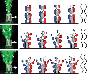
Figure 8 shows contours of normalized vorticity  $\langle \omega _z \rangle _b D/ \bar {u}_0$ and the corresponding snapshots of the instantaneous Mie scattering images for the same positions shown in figure 7. To show that the asymmetry is induced by $\Delta \varphi /{\rm \pi}$, the response is also shown at $Y = 0.5$. These correspond to planar cuts of a vortex ring wrapped around the nozzle (see Worth et al. (Reference Worth, Mistry, Berk and Dawson2020) or Gohil & Saha (Reference Gohil and Saha2019) for three-dimensional views). The trajectory of the vortices is indicated schematically by the red arrows in the particle images. At all nozzle positions, coherent structures form along the shear layer close to the nozzle exit. The images show how the forcing conditions imposed by $\hat {u}$ and $\hat {v}$ induce different patterns in which the coherent structures roll up and propagate downstream.

Figure 8. Phase-averaged vorticity ( $\langle {\omega }_z \rangle _b$) (a–d) and Mie scattering visualization (e–h) illustrating the vortex dynamics in the near field of the jet at different positions of the nozzle relative to the standing wave for $St = 0.32$ at $A = 0.15$.
At  $Y = 0$ an axisymmetric vortex ring, seen as a pair in two dimensions, forms once every forcing cycle at the nozzle exit which grows and breaks down into turbulence at the end of the potential core (Crow & Champagne Reference Crow and Champagne1971). As shown in figure 7 (and, for example, by Crow & Champagne (Reference Crow and Champagne1971) and Hussain & Zaman (Reference Hussain and Zaman1981)), this type of axisymmetric roll-up process does not lead to the separation of the jet into more than one momentum stream.
At  $Y = -1$, where the spreading rate is preferentially increased in the $x\text {--}y$ plane, vortex structures roll up in an alternating pattern once every cycle. Worth et al. (Reference Worth, Mistry, Berk and Dawson2020) showed that the three-dimensional structure provides tilted interconnected vortex rings that resemble inverted-hairpin/horseshoe vortices. However, their data only covered a small field of view ( $x/D =[0 \ \text {to} \ 4]$). Here, it is shown that at $x/D \approx 3$, the structure breaks into two smaller structures each convected along different streams towards the far field as indicated by the arrows. This leads to the separation of the jet into three momentum streams in the transverse plane similar to the structures shown by Danaila & Boersma (Reference Danaila and Boersma2000), Tyliszczak & Geurts (Reference Tyliszczak and Geurts2014) and Gohil & Saha (Reference Gohil and Saha2019).
At  $Y = \pm 0.5$, where the mean jet structure is asymmetric in the $x\text {--}y$ plane, the vortex dynamics result from a superposition of the response observed at $Y = -1$ and $Y = 0$. The axisymmetric response induced by $\hat {u}$ generates a ‘train’ of symmetric vortex rings formed once every cycle. Simultaneously, the anti-symmetric response induced by $\hat {v}$ generates an alternating vortex pattern. Since both oscillations occur at the same frequency and $\Delta \varphi /{\rm \pi} = 1$ for $Y>0$ and $\Delta \varphi /{\rm \pi} = 0$ for $Y<0$, they are superimposed and the transverse component induces the preferred direction for the axisymmetric vortex ring. This becomes evident from the vortex pattern observed at $Y = -0.5$ which is a mirror of that at $Y = 0.5$. At $Y = -0.5$, $\Delta \varphi / {\rm \pi}= 0$, which means that $\hat {u}$ and $\hat {v}$ are in phase and thus the vortex ring has a preferred direction, propagating towards $Y = 0$. At $Y = 0.5$, $\Delta \varphi /{\rm \pi} = 1$, which reverses the preferred direction towards $Y=0$ on the other side of the nozzle. This is the main difference from the study of Parekh et al. (Reference Parekh, Reynolds and Mungal1987) who force the jet longitudinally twice every transverse cycle, leading to the formation of two pairs of axisymmetric vortex rings for every transverse cycle resulting in a symmetric jet splitting into two separate momentum streams. Here, an asymmetric splitting is observed as a result of the acoustic mode.
The jet response to further combinations of  $| \hat {u} |$ and $| \hat {v} |$ is shown in figure 9 at $Y = 0.25$, $Y = 0.5$ and $Y = 0.75$. At these positions the preferred direction induced by $\Delta \varphi /{\rm \pi}$ results in a tilted jet where the vortex ring moves towards $Y = 0$. However, as the nozzle is moved closer to the velocity node at $Y = 0.25$ the asymmetry reduces and the vortex dynamics become more axisymmetric. As the nozzle is moved closer to the pressure node at $Y = 0.75$ the vortex dynamics are dominated by the anti-symmetric response as demonstrated by the alternating vortex pattern. This indicates that the response at intermediate nozzle positions can be approximated as a superposition of the symmetric and the anti-symmetric modes, depending on the position of the jet relative to $Y = 0$ and $|Y| = 1$.

Figure 9. Phase-averaged vorticity ( $\langle {\omega }_z \rangle _b$) (a–c) and Mie scattering visualization (d–f) illustrating the vortex dynamics in the near field of the jet at different positions between the pressure and velocity nodes for $St = 0.32$ at $A = 0.15$.
7. Fourier modes and modification of the base flow
To further characterize the modes excited by the acoustic fluctuations  $\hat {u}$ and $\hat {v}$ the Fourier modes $\tilde {u}$ and $\tilde {v}$ were computed using (2.1). Figure 10 shows the magnitude and phase of the modes. The top and bottom rows correspond to $\tilde {u}$ and $\tilde {v}$, respectively. The data for the modes are only shown inside the jet, where $\bar {u}/\bar {u}_0 > 0.025$, and the region outside is shaded in grey. The first two columns correspond to the symmetric mode at $Y = 0$, the second to the mixed mode at $Y = 0.5$ and the third to the anti-symmetric mode at $Y = 1$. The phase contours indicate the patterns of convective propagation where a quantity, e.g. $\tilde {u}$, is convected along the gradient of the phase map. The symmetric mode at $Y = 0$ is characterized by an anti-symmetric pattern of the phase $\angle (\tilde {v})$ and a symmetric pattern of $\angle (\tilde {u})$ with respect to the nozzle centreline. This is a feature of the propagation of the axisymmetric vortex rings shown in the previous section. The anti-symmetric mode at $Y = 1$ is characterized by a symmetric pattern of $\angle (\tilde {v})$ and an anti-symmetric pattern of $\angle (\tilde {u})$. This is indicative of the alternating vortex pattern shown in the previous section. At the mixed position $Y = 0.5$ the structures of $\tilde {u}$ and $\tilde {v}$ contain features of both the symmetric and anti-symmetric modes which are utilized next.

Figure 10. Fourier modes  $\tilde {u}$ and $\tilde {v}$ for $St = 0.32$ at $A = 0.15$ showing the symmetric mode at $Y = 0$, a mixed mode at $Y = 0.5$ and the anti-symmetric mode at $Y = 1$. The black dashed lines indicate the jet boundary where $\bar {u}/\bar {u}_0 = 0.025$. All images are shown in the region $x/D = [0.5 \ \text {to} \ 7]$ and $y/D = [-3.5 \ \text {to} \ 3.5]$.
The transverse acoustic velocity  $|\hat {v}|$ is estimated by averaging $|\tilde {v}|$ in the region $x/D = [10 \ \text {to} \ 14]$ and $y/D = [-1 \ \text {to} \ 1]$. The normalized velocity $|\hat {v}| \rho c / \hat {p}_T$ from the MMM and PIV was shown to be in good agreement in figure 2 for all values of $A$,
$A$,  $Y$ and $St$, showing that for $x/D>10$, $\tilde {v}$ is reduced to the transverse acoustic velocity $\hat {v}$. However, in the near field $\tilde {v}$ differs significantly from the one-dimensional acoustic mode shape given by (4.1a,b). Next, it is demonstrated that the manipulated boundary conditions, i.e. the jet exit profiles at $x/D =1$ of $\tilde {u}$ and $\tilde {v}$, at mixed positions are linear combinations of the symmetric and anti-symmetric boundary conditions measured at $Y = 0$ and $Y = 1$.
The jet exit boundary conditions at  $x/D = 1$ are shown in terms of the r.m.s. ( $u_{rms}$ and $v_{rms}$) and Fourier mode profiles ( $| \tilde {u} |$ and $| \tilde {v} |$) in figure 11 for $St= 0.32$ at all nozzle locations for $A = 0.15$. Figure 11(a,e,i,m) shows the profiles at $Y = 0$ and $Y = 1$ corresponding to boundary conditions for the symmetric and anti-symmetric modes. As a reference, the r.m.s. profiles are shown for the unforced case. All r.m.s. values are multiplied by a factor $\sqrt {2}$ to compare with the harmonic amplitudes of the modes. The magnitude of all Fourier mode profiles are similar to the r.m.s. profiles indicating that most of the energy and thus most of the flow dynamics are captured by the modes. The discrepancies between the Fourier modes and r.m.s. are mainly observed in the shear layer and are of the same order of magnitude as the r.m.s. measured in the unforced case. As mentioned before, at $Y = 0$ a symmetric pattern is observed for $\tilde {u}$ and an anti-symmetric pattern is observed for $\tilde {v}$, whereas the opposite is seen at $Y = 1$. This symmetry and anti-symmetry in the boundary conditions is not visible in the profiles, since it is contained in the phase distribution of the modes as shown in figure 10. At $Y = 0$, $|\tilde {u}|$ is increased at the jet centreline proportional to $\hat {u}$ measured by the MMM where $\sqrt {2} u_{rms}/\bar {u}_0 \approx | \tilde u|/\bar {u}_0 \approx A \approx 0.15$. At $Y = 1$, $|\tilde {u}|$ is similar to the unforced profile and $|\tilde {v}|$ is increased significantly across the jet. Note that the magnitude of $| \tilde v|/\bar {u}_0$ is significantly larger than the magnitude of the transverse acoustic velocity $| \hat {v} |$. These two sets of boundary conditions induce different motions of the potential core which are discussed in the last part of this section.

Figure 11. Jet exit boundary conditions in terms of root mean square (r.m.s.) fluctuations (a–d,i–l) and Fourier mode profiles (e–h,m–p) shown at  $x/D = 1$ for $A = 0.15$ at $St = 0.32$. (a,e,i,m) Boundary conditions for the symmetric ( $Y= 0$) and anti-symmetric ( $Y= 1$) modes, and for the unforced jet. (b,f,j,n,c,g,k,o,d,h,l,p) Boundary conditions measured at the intermediate positions and the solid lines show reconstructed mixed modes from superposition of the symmetric and anti-symmetric profiles. All the measured profiles contain uncertainties of $\Delta / \bar {u}_0 \approx \pm 0.02$, and the reconstructed profiles contain $\Delta / \bar {u}_0 \approx \pm 0.04$.
At the intermediate locations all profiles are skewed with respect to the nozzle centreline where  $|\tilde {u}|$ and $|\tilde {v}|$ are significantly increased in the direction $y/D<0$ for $Y>0$. This is due to a superposition of the boundary conditions at $Y = 0$ and $Y = 1$ leading to an asymmetric profile. This asymmetry is symmetric with respect to the velocity node, and is shown in figure 11(c,g,k,o) with the profiles for both $Y = -0.5$ and $Y = 0.5$. At $Y = -0.5$ the skewed profiles show increased fluctuations at $y/D>0$ caused by a change of the phase $\Delta \varphi /{\rm \pi}$ by half a cycle.
We now consider whether the boundary conditions at  $0 < Y < 1$ and $-1 < Y < 0$ can be well approximated by linear combinations of the symmetric and anti-symmetric boundary conditions at $Y = 0$ and $|Y| = 1$. In figure 6 it is shown that the amplitude and phase of the acoustic fluctuations $\hat {u}$ and $\hat {v}$ at a given $Y$ position change as a function of the pressure and velocity in a standing wave. Hence, the proportionalities in (4.2a,b) can be utilized as weighting functions where the profiles $\tilde {u}^Y_p(y)$ and $\tilde {v}^Y_p(y)$ at an intermediate position $Y$ can be approximated by
 \begin{gather} \tilde{u}^Y_p(y) = \tilde{u}^{Y_0}(y) \cos{\left( {\rm \pi}/2 Y \right)} \frac{\hat{p}^{Y}_T}{\hat{p}^{Y_0}_T} + \tilde{u}^{Y_1}(y) \sin{\left( {\rm \pi}/2 Y \right)} \frac{\hat{p}^{Y}_T}{\hat{p}^{Y_1}_T}, \end{gather}
 \begin{gather}\tilde{v}^Y_p(y) = \tilde{v}^{Y_0}(y) \cos{\left( {\rm \pi}/2 Y \right)} \frac{\hat{p}^{Y}_T}{\hat{p}^{Y_0}_T} + \tilde{v}^{Y_1}(y) \sin{\left( {\rm \pi}/2 Y \right)} \frac{\hat{p}^{Y}_T}{\hat{p}^{Y_1}_T}, \end{gather}
where  $\tilde {u}^{Y_0}(y)$, $\tilde {u}^{Y_1}(y)$, $\tilde {v}^{Y_0}(y)$ and $\tilde {v}^{Y_1}(y)$ are jet exit profiles of the Fourier modes $\tilde {u}$ and $\tilde {v}$ measured at $Y = 0$ and $Y = 1$. From these profiles the harmonic time evolution can be obtained from (2.1). The profiles used for the reconstructions here are the ones shown at $x/D = 1$ in figure 11(a,e,i,m). The pressure ratios, $\hat {p}^{Y}_T/\hat {p}^{Y_0}_T \approx 1$ and $\hat {p}^{Y}_T/\hat {p}^{Y_1}_T \approx 1$, account for the differences in the maximum pressure level in the box between measurements. Ideally these two ratios are one and are only added to the equation to account for experimental differences in $A$ between the measurements. The weights $\cos {( {\rm \pi}/2 Y )}$ and $\sin {( {\rm \pi}/2 Y )}$ are proportional to the acoustic fluctuations $\hat {u}$ and $\hat {v}$ in the standing wave. At $Y = 0$, $\tilde {u}^Y_p$ becomes $\tilde {u}^{Y_0}$, at $Y = 1$, $\tilde {u}^Y_p$ becomes $\tilde {u}^{Y_1}$, and at $0 < Y < 1$ and $-1 < Y < 0$, $\tilde {u}^Y_p$ becomes a superposition of the two whose weights depend on the position in the standing wave. The magnitudes of the reconstructed boundary conditions $|\tilde {u}^Y_p|$ and $|\tilde {v}^Y_p|$ are overlaid at all intermediate locations in figure 11 as red lines and show good agreement with the measured ones, $|\tilde {u}|$ and $|\tilde {v}|$. This shows that the jet exit boundary conditions at $0 < Y < 1$ and $-1 < Y < 0$ are well approximated as a linear combination of the boundary conditions of the symmetric and anti-symmetric modes measured at $Y = 0$ and $Y = 1$. This also indicates that the acoustic forcing is an inviscid effect primarily altering the jet exit boundary conditions, which leads to linear amplification of convective modes. It also shows that when superimposing $m=0$ and $m=\pm 1$ forcing at $r_f = 1$ the result is an asymmetry in the base flow that develops into the asymmetric dynamics presented in the previous section.
The reconstructions in figure 11 are only shown for  $St = 0.32$ and $A = 0.15$. To quantify errors of the reconstruction and to demonstrate that it works for all values of $St$,
$St$,  $A$ and $Y$, we compute relative errors, using
 \begin{equation} \tilde{u}_e = \frac{\left|\tilde{u} \right|- \left|\tilde{u}^Y_p \right|}{\left|\tilde{u} \right|+ \left|\tilde{u}^Y_p \right|}, \quad \tilde{v}_e = \frac{\left|\tilde{v} \right|- \left|\tilde{v}^Y_p \right|}{\left|\tilde{v} \right|+ \left|\tilde{v}^Y_p \right|}, \end{equation}
for all measurements. The relative errors are computed across the nozzle, i.e.  $y/D = [ -0.5 \ \text {to} \ 0.5]$, and are shown as histograms in figure 12. The average errors are $2\,\%$ and $1\,\%$ and the standard deviations are $27\,\%$ and $14\,\%$ for $\tilde {u}^Y_p$ and $\tilde {v}^Y_p$ respectively. The errors are slightly larger for $\tilde {u}^Y_p$ due to the influence of the shear layer. However, the procedure works reasonably well at all operating points and the skewness of the profiles is well captured.

Figure 12. Histograms of relative errors  ${\tilde {u}_e}$ and ${\tilde {v}_e}$ for all jet exit profiles computed across the nozzle $y/D = [ -0.5 \ \text {to} \ 0.5]$ at $x/D = 1$. The mean error and standard deviation are $3\,\%$ and $27\,\%$ for $\tilde {u}_e$ and $1\,\%$ and $14\,\%$ for $\tilde {v}_e$ respectively.
The asymmetric forcing observed at  $0 < Y < 1$ and $-1 < Y < 0$ has the effect of deflecting the jet away from its geometric centre as shown in figures 7, 8 and 9. This can also be captured by reconstructing the time series of vorticity and velocity using (2.2), as shown in figure 13. Contours of the velocity magnitude $| \boldsymbol {\langle u \rangle _{F}} | = \sqrt { \langle u \rangle ^2_{F} + \langle v \rangle ^2_{F} }$ indicating the potential core (grey) and vorticity $| \langle \omega _z \rangle _{F} | D /\bar {u}_0 > 1$ (red and blue) show the evolution of the coherent structures.

Figure 13. Time series reconstructed from the Fourier modes using (2.2) for  $St = 0.32$ at all nozzle locations indicating the dynamics of the potential core and the induced vortex dynamics. The black and grey contours indicate $| \langle \boldsymbol {u} \rangle _{F} |/\bar {u}_0 > 0.8$. The red and blue contours indicate $| \langle \omega _z \rangle _{F} | D /\bar {u}_0 > 1$. The data are shown for $A = 0.15$ but the dynamics are similar at all $A$ and for both $St$.
$St$.
At  $Y = 0$ the axisymmetric mode, $m = 0$, occurs with the potential core deforming into regions of high and low velocity accompanied by the axisymmetric roll-up of coherent structures. At $Y = 1$ the potential core is periodically deflected generating a sinuous shape resulting in an alternating pattern of vortices. These vortices continue to propagate towards the far field significantly increasing the jet spreading rate which is quantified in the next sections. As the nozzle is moved from $Y = 0$ towards $Y = 1$, the jet transitions from the symmetric to anti-symmetric modes, $m = 0$ to $m =\pm 1$. At $Y = 0.25$ significant asymmetry in the vorticity fields is evident and when placed at $Y = 0.75$ show a clear bifurcation. The effect is mirrored if the jet is traversed in the $-Y$ direction as shown at $Y = -0.5$ due to the change of $\Delta \varphi /{\rm \pi}$ by half a cycle between $\hat {u}$ and $\hat {v}$.
The effect of  $St$ is depicted in figure 14 with Mie scattering images, and $| \boldsymbol {\langle u \rangle _{F}} |$ and $| \langle \omega _z \rangle _{F} |$ reconstructed from the Fourier modes for both $St = 0.32$ and $St = 0.47$. Contours are added at $\bar {u}/\bar {u}_0 = 0.025$ to indicate the jet boundary and the streamwise velocity profiles are included at $x/D = 8$. The two images in figure 14(a,b) have been processed to highlight the edges of the potential core in order to show the jet boundary, growth and relative positioning of the coherent structures. The spreading rate is significantly greater for $St = 0.32$ compared with $St = 0.47$ consistent with the observations by Gohil & Saha (Reference Gohil and Saha2019). Increasing spreading rates occur closer to the preferred mode where the forcing is most amplified. This leads to an optimal spacing between coherent structures. Compared with $St = 0.32$, the separation between coherent structures is smaller at $St = 0.47$ due to the higher frequency shown by labels A and C. Location A shows where the primary structure breaks into two smaller structures and C indicates their downstream trajectories. For $St = 0.32$, the same event is labelled B and D, respectively, where the coherent structures split into two smaller structures that propagate downstream in different directions. These effects are captured by the reconstructed time series in figure 14(c). The difference in separation and direction leads to significantly different profiles shown by the velocity profiles at $x/D = 8$. At $0^{\circ }$ the events A–D are also labelled showing that the wider profile is a direct result of the increased angle of the separated structure as it propagates towards the far field when $St = 0.32$.

Figure 14. Influence of increased forcing frequency at  $Y = 1$ for $A=0.15$. (a,b) Processed Mie scattering images illustrate the separation and growth of coherent structures and indicate the boundary of the potential core. (c) Contours for $| \boldsymbol {\langle u \rangle _{F}} |$ and $| \langle \omega _z \rangle _{F} | D /\bar {u}_0 > 1$ similar to what is shown in figure 13. Contours of $\bar {u}/\bar {u}_0 = 0.025$ (black solid line) are added to indicate the spreading rate and the streamwise velocity profile $\bar {u}/\bar {u}_0$ (grey solid line) is shown at $x/D = 6$.
8. Time-averaged jet development
In the previous sections, it was shown that the dynamics in the near field of the jet depends on the position of the nozzle with respect to the standing wave. Furthermore, the boundary conditions leading to the mixed modes are well approximated by a linear combination of the boundary conditions for the symmetric and anti-symmetric modes. In this section the time-averaged flow fields  $\bar {u}$, $\bar {v}$ and $\bar {\omega }_z$ are presented to show their influence on the developing region of the jet.
Figure 15 shows the time-averaged flow fields for all positions and forcing levels at  $St = 0.32$ in the range $x/D = [0 \ \text {to} \ 20]$. Normalized vorticity $\bar {\omega }_z D /\bar {u}_0$ is given by the colour map and the contours of constant streamwise velocity $\bar {u}/\bar {u}_0$ show how the jet develops downstream.

Figure 15. Time-averaged flow fields showing the average jet structure at all operating conditions for  $St = 0.32$. The colour map shows normalized vorticity $\bar {\omega }_z D /\bar {u}_0$ indicating the shear layers. The contours correspond to regions of constant streamwise velocity $\bar {u}/\bar {u}_0$ indicating the outer boundary of the jet (black dashed line) and the development of the potential core (black solid line) towards the far field.
At  $Y = 0$ the jet is similar to the unforced case. As the forcing level is increased the mean shape and structure of the jet remain approximately axisymmetric. The differences observed at $A = 0.25$ are due to a small but increasing value of $|\hat {v}|$ due to imperfect alignment of the nodal line with the centre of the nozzle. This shows that the jet is very sensitive to transverse oscillations.
The sensitivity to  $\hat {v}$ becomes evident when $Y>0$. Already at $Y = 0.25$ a significant increase in the spreading rate is observed. The asymmetric dynamics shown in the previous sections leads to preferential spreading of the jet towards $|Y|=1$ whilst the jet centreline is deflected in the opposite direction towards $Y=0$. The same behaviour is observed for all intermediate positions where the jet centreline is tilted left for $Y>0$ and right for $Y<0$. Although the forcing conditions and dynamics at $Y = 0.25$ and $Y = 0.75$ are different, the time-averaged structure of the jets appears similar at the same forcing level. As the jet is moved towards $| Y | = 1$ the profiles of $\bar {u}/\bar {u}_0 = 0.3$ show reduced skewness becoming symmetric at $| Y | = 1$. As $A$ is increased the profiles of $\bar {u}/\bar {u}_0 = 0.5$ split into two or more streams indicative of a ‘bifurcated’ jet (Reynolds et al. Reference Reynolds, Parekh, Juvet and Lee2003). This separation into two streams is stronger at $St = 0.32$ compared to $St = 0.47$ which is not shown here for brevity.
At  $|Y| = 1$ the spreading rate is significantly increased and is symmetric across the jet centreline. As $A$ is increased the jet splits into three momentum streams similar to the ‘ $\varPsi$’ jet observed in Danaila & Boersma (Reference Danaila and Boersma2000) and Gohil & Saha (Reference Gohil and Saha2019). We can also obtain the bifurcation angles $\Delta \beta$ at $Y=1$ to compare with the numerical simulation of Gohil & Saha (Reference Gohil and Saha2019). Using their methodology, we track the jet boundary corresponding to isocontours of $\bar {u}/\bar {u}_0=0.1$ of the mean fields shown in figure 15 which results in ‘bifurcation angles’ of $\Delta \beta \approx 65^\circ$ for $St= 0.32$ and $\Delta \beta \approx 35^\circ$ for $St= 0.47$ which are in excellent agreement with the results of Gohil & Saha (Reference Gohil and Saha2019). However, the use of $\Delta \beta$ to characterize the spreading rate is not suitable for asymmetric velocity profiles as shown in figure 16 and in numerous previous studies (e.g. da Silva & Métais Reference da Silva and Métais2002; Tyliszczak Reference Tyliszczak2015; Gohil & Saha Reference Gohil and Saha2019) and we therefore propose an alternative approach based on a statistical analysis of the streamwise momentum presented in the next section.

Figure 16. Velocity profiles at  $x/D = 10$ for $St = 0.32$ at $A = 0.15$. (a) Streamwise velocity $\bar {u}/\bar {u}_0$. (b) Transverse velocity $\bar {v}/\bar {u}_0$. The wider profiles indicate an increased spreading rate.
As shown for  $Y = 1$ in figure 14, the structure of the jet is similar for similar positions at both $St$. However, the spreading rate and strength of the jet splitting is significantly lower for $St = 0.47$ for all positions and forcing levels as they are away from the preferred mode.
To highlight bifurcation or splitting of the jet from a single momentum stream, the mean streamwise and transverse velocity profiles are shown in figure 16 for  $A = 0.15$ at $x/D = 10$. For brevity profiles are only shown for $St = 0.32$ noting that similar profiles were observed for $St = 0.47$ but with a reduced spreading rate. Figure 16(a) shows profiles of $\bar {u}/\bar {u}_0$. Figure 16(b) shows profiles of $\bar {v}/\bar {u}_0$. At $Y = 0$ profiles of $\bar {u}/\overline {u_0}$ and $\bar {v}/\overline {u_0}$ are similar to the unforced case. At $Y = 1$ the $\bar {u}/\overline {u_0}$ profile shows a symmetric distribution characterized by three peaks with maximum velocity at the nozzle centreline. The corresponding profile $\bar {v}/\overline {u_0}$ shows that both sides contain a significant $\bar {v}$ component. This indicates that the jet has separated into three separate momentum streams and is very similar to the ‘ $\varPsi$’ jet in Gohil & Saha (Reference Gohil and Saha2019).
Figure 17 compares the response at  $Y=1$ with Gohil & Saha (Reference Gohil and Saha2019) and $Y=0.75$ with Longmire & Duong (Reference Longmire and Duong1996). Figure 17(a,b) plots velocity profiles at various downstream locations and Strouhal numbers for the $Y=1$ case. Overall, good agreement for both Strouhal numbers is found indicating the jet response is similar in both instances. Excellent agreement at $Y=0.75$ with Longmire & Duong (Reference Longmire and Duong1996) is also found in figure 17(c).

Figure 17. Comparison of velocity profiles  $\bar {u}/\bar {u}_0$ against those reported in Gohil & Saha (Reference Gohil and Saha2019) and Longmire et al. (Reference Longmire, Eaton and Elkins1992) for similar conditions. (a,b) Profiles for $x/D = [6,10]$ at $Y = 1$ for $A = 0.15$: (a) $St = 0.32$ compared against $St = 0.3$ and (b) $St = 0.47$ compared against $St = 0.5$. (c) Profile for $x/D = 4$ for $A = 0.15$ at $Y = 0.75$ compared against the profile produced by the forced step nozzle in Longmire & Duong (Reference Longmire and Duong1996).
Finally, we consider the effect of the jet position and forcing amplitude on the relative change to the normalized momentum thickness  $\theta /\theta _0$ as plotted in figure 18. These were evaluated from the PIV data at $x/D=1$ as hot wire measurements were not conducted for all operating conditions investigated. Figure 18(a) shows that the spreading rate increases with $A^* = A \ {\hat {p}^{Y}_T}/{\hat {p}^{Y_0}_T}$ due to the formation of larger structures. Figure 18(b) shows the effect of amplitude and jet position on $\theta /\theta _0$. Increasing $A$ results in an approximately linear increase in $\theta /\theta _0$ up to approximately $A^*=0.25$. At $Y>0$ it appears that the response becomes nonlinear at lower amplitudes.

Figure 18. Effect of forcing on the momentum thickness  $\theta$ computed at $x/D = 1$. (a) The velocity profile at $Y=0$ against $A$. (b) The momentum thickness $\theta /\theta _0$ relative to the unforced case against the pressure-corrected forcing amplitude $A^* = A \ {\hat {p}^{Y}_T}/{\hat {p}^{Y_0}_T}$.
Overall, the results and comparisons in this section illustrate that transverse acoustic forcing leads to a family of ‘bifurcated’ jets in the transverse plane. This planar splitting of the jet is very similar to previous ‘bifurcated’ jets produced by active or passive forcing but with some important differences. The forcing is monochromatic,  $r_f = 1$, and the forcing components are varied by the jet's relative location within the standing wave which has not been explored before to the best of the authors’ knowledge.
9. Statistical analysis of the streamwise momentum
In the following sections, two new methods to characterize the degree of bifurcation are presented. First, the jet is characterized based on the development of the statistical behaviour of the streamwise momentum downstream. Then, in the next section, a model is proposed to identify the number of individual momentum streams.
To characterize the modified behaviour of the forced jets statistically, p.d.f.s of streamwise momentum  $f_{{M}}$ are constructed from profiles of the streamwise velocity field, where
 \begin{equation} f_{{M}} = \dfrac{\rho \bar{u}(x,y)^2}{\rho \displaystyle\int_{-\infty}^{\infty} \bar{u}(x,y)^2\, \mathrm{d}y}. \end{equation}
The  $n^{({\rm th})}$ statistical moment $\mu _n$ of $f_{{M}}$ was computed using
 \begin{equation} \mu_n =\int_{-\infty}^{\infty} \left( y - C_{{M}} \right)^n f_{{M}} \,\mathrm{d}y, \end{equation}
where  $n=1$ gives the centre of momentum, $C_{M}$, $n=2$ gives the variance, $V_{M} = \sigma _{M}^2$, indicating the spreading rate, and $n=3$ gives the skewness, $S_{M}$, indicating departure from symmetry. Figure 19 shows $f_{{M}}$ at $x/D = 10$ for $Y= [-1,-0.5,0]$ for $A = 0.15$ at $St = 0.32$. The insets show an image of $f_{{M}}(x,y)$ which appears as a collection of p.d.f.s in the region $y/D = [-7 \ \text {to} \ 7]$ and $x/D = [1 \ \text {to} \ 24]$. In the image of $f_{{M}}(x,y)$ all p.d.f.s are normalized by the maximum value $\text {max}_x(\, f_{{M}} )$ to highlight the trajectories of momentum. In the main figures the profiles of $f_{{M}}$ are shown at $x/D = 10$ corresponding to the red lines in the insets. The dashed lines indicate the centre of momentum, $C_{M}$, and $C_{M} \pm 3\sigma _{M}$.

Figure 19. The p.d.f.s of streamwise momentum  $f_{{M}}$ shown at $x/D= 10$ (red solid line) for $A = 0.15$ and $St = 0.32$. The dot-dashed lines indicate the location of $C_{{M}}$ and $C_{{M}} \pm 3 \sigma _{{M}}$. The insets show $f_{{M}}(x,y) / \max _x(\, f_{{M}} )$ coloured by magnitude in the region $y/D = [-7 \ \text {to} \ 7]$ and $x/D = [1 \ \text {to} \ 24]$ where each p.d.f. is normalized by the maximum value $\max _x(\, f_{{M}} )$. (a) Pressure node $(Y = -1)$ characterized by a symmetric distribution containing three peaks. (b) Intermediate position $(Y = -0.5)$ characterized by an asymmetric distribution containing two peaks. (c) Velocity node $(Y = 0)$ characterized by a symmetric distribution containing a single peak.
At  $Y = 0$ the shape of $f_{M}$ is approximately Gaussian, characterized by $S_{M} \approx 0$ and a $95\,\%$ confidence interval of $6\sigma _{M}$. At $Y = -1$ and $Y = -0.5$, $f_{{M}}$ is clearly not well represented by a single Gaussian distribution. At $Y = -1$, $f_{{M}}$ contains three distinct peaks and is approximately symmetric ( $S_{M} \approx 0$) with respect to $C_{M}$. At $Y = -0.5$ the distribution is asymmetric ( $S_{M} < 0$) and $f_{{M}}$ contains two peaks. The asymmetry is also shown by the different lengths between $C_{M} \pm 3\sigma _{M}$ and the tails of $f_{{M}}$ on each side.
The moments  $C_{M}$, $\sigma _{M}$ and $S_{M}$ are computed in the region $x/D = [1 \ \text {to} \ 24]$ which are plotted in figure 20. The figure shows the downstream development of the moments for $St=0.32$ and $A = 0.05$ at different positions $Y$. The red lines show the unforced case which is added for reference.

Figure 20. Development of statistical moments for  $St = 0.32$ and $A = 0.05$: (a) $C_{M}$, (b) $\sigma _{M}/\sigma _{{M}_0}$ and (c) $S_{M}$. The inset in (b) shows $3 \sigma _{{M}_0}/D$ for the unforced jet which has an average spreading angle $\theta _{{M}_0} = 8.2^{\circ }$. Moment $S_{M}$ is normalized by $x^2$ to account for the linear spreading rate.
Figure 20(a) shows that  $| C_{M}/D |<1$ for all positions. This result indicates that the centre of momentum is located along the nozzle centreline and shows that introducing transverse forcing does not alter the location of the average streamwise momentum. The same observation is made for the other values of $A$ and $St$, which are not shown for brevity.
Figure 20(b) shows  $\sigma _{M}$ normalized by $\sigma _{{M}_0}$ which is computed for the unforced jet. Here $\sigma _{{M}_0}$ develops linearly as shown in the inset and the average spreading angle of momentum is $\theta _{{M}_0} = 8.2^{\circ }$. In § 3 it was verified that the unforced jet is self-similar with a half-width $y_0 = 0.095$. In this way, the lines in figure 20(b) show the spreading rate of momentum relative to the unforced case. At $Y = 0$ the jet develops similarly to the unforced case. For all cases where $|\hat {v}|>0$, $\sigma _{M}/\sigma _{{M}_0}$ increases rapidly in the region $x/D = [2 \ \text {to} \ 8]$ before it levels off and starts to decrease slowly. This indicates that the spreading of momentum increases linearly with $x$ albeit at a significantly larger rate than the unforced case. This rapid increase of the spreading rate for $x/D > 2$ is consistent with the ‘bifurcation point’ usually reported in the range $x/D = [2 \ \text {to} \ 4]$, e.g. as reported in Suzuki et al. (Reference Suzuki, Kasagi and Suzuki2004). The slow decrease of $\sigma _{M}/\sigma _{{M}_0}$ at $x/D>10$ indicates that after the jet splits, the centreline of each momentum stream slowly restores itself towards a more streamwise orientation as it develops. This slow change in orientation is captured by the method proposed in the next section.
For comparison, the average relative spreading rate  $\bar {\sigma }_{M} / \bar {\sigma }_{{M}_0}$ is computed at $x/D > 10$. Figure 21(a) shows $\bar {\sigma }_{M} / \bar {\sigma }_{{M}_0}$ at different $Y$,
$Y$,  $A$, and $St$. The variation of $\bar {\sigma }_{M} / \bar {\sigma }_{{M}_0}$ with $Y$ closely follows the variation of $| \hat {v} |$. Therefore $\bar {\sigma }_{M} / \bar {\sigma }_{{M}_0}$ can also be fitted to (4.2a,b) for each $St$ and is shown in black lines. The amplitudes of the black lines are obtained by fitting $\bar {\sigma }_{M} / \bar {\sigma }_{{M}_0}$ to (4.2a,b) for each $St$ separately which includes the variation due to different forcing levels. The coloured regions indicate $95\,\%$ confidence intervals. The fits give $\bar {\sigma }_{M} / \bar {\sigma }_{{M}_0} \approx 2.7 \pm 0.2$ for $St = 0.32$ and $\bar {\sigma }_{M} / \bar {\sigma }_{{M}_0} \approx 1.8 \pm 0.1$ for $St = 0.47$. These show that there is a significant difference between the two frequencies even after including the variation in forcing amplitude. Furthermore, the increased spreading rate is found to be more sensitive to the forcing frequency than to the forcing level as would be expected when the jet is forced closer to the preferred mode. For instance, the spreading rate is larger for $St = 0.32$ at $A=0.05$ compared with $St = 0.47$ at $A=0.25$ even though the latter is forced with a magnitude five times larger. Hence, the difference is unlikely to be due to the $20\,\%$ difference in the ratio between $|\hat {u}|$ and $|\hat {v}|$, which was shown in § 4 to be an acoustic feature of the rig.

Figure 21. (a) Average relative momentum spreading rate  $\bar {\sigma }_{M} / \bar {\sigma }_{{M}_0}$ and (b) average symmetry $\bar {S}_{M}$ in the far field $x/D>10$ at different nozzle positions. In (a), the black solid lines indicate fits of $\bar {\sigma }_{M} / \bar {\sigma }_{{M}_0}$ to (4.2a,b) which is proportional to $|\hat {v}|$. The scatter is indicated by the coloured regions. The variation of $\bar {\sigma }_{M} / \bar {\sigma }_{{M}_0}$ due to the change in $A$ is significantly smaller than the variation due to the change of $St$. In (b), the black solid lines indicate fits of $\bar {S}_{M}$ to the product $\hat {u} \hat {v} \propto \sin {( {\rm \pi}/2 Y )} \cos {( {\rm \pi}/2 Y )}$. The asymmetry increases with $A$ and is proportional to the product of $\hat {u}$ and $\hat {v}$ where $\bar {S}_{M}<0$ for $Y < 0$ and $\bar {S}_{M}>0$ for $Y > 0$.
The skewness  $S_{M}$ is shown in figure 20(c) normalized by $x^2$ to compensate for the linear spreading rate. It is evident that $S_{M}/x^2>0$ for $Y>0$ and $S_{M}/x^2<0$ for $Y<0$. The initial development is similar to $\sigma _{M}/\sigma _{{M}_0}$ where $S_{M}/x^2$ increases rapidly in the region $x/D = [2 \ \text {to} \ 8]$ before it levels off and slowly decreases. At $Y = 1$ and $Y = 0$, $S_{M}/x^2 \approx 0$ and hence the jet develops symmetrically. This shows that the asymmetry at the intermediate locations is caused by the asymmetry in forcing across the jet nozzle.
To compare the symmetry for different forcing levels and positions  $\bar {S}_{M}$ is computed similarly to $\bar {\sigma }_{M} / \bar {\sigma }_{{M}_0}$ by taking the average at $x/D > 10$. Figure 21(b) shows $\bar {S}_{M}$ at different $Y$ and $A$. For brevity data are only shown for $St = 0.32$. The variation of $\bar {S}_{M}$ with $Y$ is similar to the product of $\hat {u} \hat {v}$ given by $\sin {( {\rm \pi}/2 Y ) }\cos {( {\rm \pi}/2 Y ) }$ which is fitted to the data at each value of $A$ and are shown by the solid lines. At $|Y| = 1$ and $Y = 0$, $\bar {S}_{M} \approx 0$ for most operating points. However, at this location a significant value of $\bar {S}_{M}$ is observed at high forcing levels, e.g. at $Y = -1$ for $A = 0.25$. This is believed to be due to imperfect alignment with the nodal line and the jet centreline resulting in small asymmetries due to the absence of both $\hat {u}$ and $\hat {v}$. However, the fits provide amplitudes $\bar {S}_{M} = [0.020\pm 0.004 ,0.036\pm 0.016, 0.077\pm 0.047]$. Dividing the fitted amplitudes by $A$ yields $\bar {S}_{M}/A = [ 0.39\pm 0.08 , 0.25\pm 0.11 , 0.31\pm 0.19]$ showing that the symmetry is proportional to $A$.
$A$.
In this section the jets are characterized by the development of statistical moments of the streamwise momentum in terms of the centre of momentum, the spreading rate and the symmetry. This method provides an alternative way to characterize the jets rather than labelling the jets based on the number of ‘branches’. However, an interesting question still remains. The velocity profiles downstream clearly indicate a ‘bifurcation’, i.e. separation into separate momentum streams. If the jet ‘bifurcates’, do each of these streams behave like a self-similar jet in the far field? In the next section this question is investigated by proposing a method to isolate each momentum stream from the measurements. Then each branch is analysed individually using a similar approach to that taken when studying the unforced case.
10. Number of momentum streams and self-similarity
To decompose the jet into separate momentum streams, profiles of the streamwise velocity  $\bar {u}$ are fitted to a sum of Gaussian profiles given by
 \begin{equation} \bar{u}_t(x,y) = \sum_{i=1}^{n_g} \bar{u}_i = \sum_{i=1}^{n_g} a_i(x) \exp{ \left( \ln{\left( 0.5 \right)} \left( \frac{y-b_i(x)}{c_i(x)}\right)^2 \right)}. \end{equation}
Here  $\bar {u}_t$ is a slice of the total streamwise velocity represented as a sum of $n_g =1$, $n_g =2$ or $n_g =3$ velocity profiles. Each profile represents a momentum stream and is described by $\bar {u}_i$. The parameters $a_i(x)$ and $c_i(x)$ are similar to $\bar {u}_{\max }$ and $y_0$ in (3.2), respectively, and $b_i(x)$ is the centreline position of the profile. Therefore, $b_i(x)$ accounts for the separation between the nozzle centreline $y/D = 0$ and the jet centreline of each momentum stream $\bar {u}_i$. Equation (10.1) is fitted to $\bar {u}$ in the range $x/D = [4 \ \text {to} \ 24]$; hence $\bar {u}_t(x,y)$ is the reconstructed velocity field in terms of Gaussian profiles.
The result of the method is depicted in figure 22. This corresponds to the jet located at  $Y = 0.75$, $St = 0.32$ and $A = 0.15$ corresponding to a condition where the jet clearly splits into two momentum streams; hence $n_g = 2$ is chosen. Figure 22(a–c) shows contours of constant streamwise velocity described by $\bar {u}_1$, $\bar {u}_2$ and their sum $\bar {u}_t$, respectively. Figure 22(d) shows the jet centrelines $b_1(x)$ and $b_2(x)$ for both momentum streams where the dashed line indicates the nozzle centreline. Figure 22(e) shows the profiles along the lines $x/D = 10$ in figure 22(a–c), and the PIV measurements $\bar {u}$ are shown in red circles. There is an excellent agreement between the fit and the measurements indicating that the model captures the velocity field. Notice that $| b_2(x) | > | b_1(x) |$ and $a_1(x) > a_2(x)$. The trajectories of $b_1(x)$ and $b_2(x)$ shown in figure 22(d) also indicate that the jet centrelines are starting to restore towards a more streamwise orientation for $x/D>10$. This explains the slowly reducing trends of the momentum spreading rate $\sigma _M/\sigma _{M_0}$ shown in figure 20. The left-hand stream contains a higher centreline velocity when compared with the right-hand stream which is a result of the preferred direction induced by the acoustic fluctuations. Their sum results in an asymmetric bifurcation.

Figure 22. Reconstruction of  $\bar {u}$ at $Y = 0.75$ and $A = 0.15$ by superposition of $n_g = 2$ Gaussian profiles. Contours of constant streamwise velocity for (a) the left-hand momentum stream $\bar {u}_1/\bar {u}_0$, (b) the right-hand momentum stream $\bar {u}_2/\bar {u}_0$ and (c) the sum of both streams $\bar {u}_t/\bar {u}_0$. (d) Streamwise trajectories of the jet centrelines $b_1(x)$ and $b_2(x)$ for the two momentum streams. (e) Profiles of streamwise velocity at $x/D = 10$. The profiles are shown along the lines indicated in (a–c).
The excellent agreement of the expression given by (10.1) with the measurements provides an alternative method to classify a number of separated momentum streams which is shown next. The method is used to classify if the jet consists of one, two or three momentum streams. First, relative errors  $\bar {u}_e$ are computed between the model and the measurements:
 \begin{equation} \bar{u}_e = \frac{\bar{u}_t - \bar{u}}{\bar{u}_{max}}. \end{equation}
The normalization by  $\bar {u}_{max}$ is used to avoid amplified errors due to low velocities outside of the jet where $\bar {u}/\bar {u}_0$ approaches zero. In this way, lower values of $\bar {u}_e$ indicate better fits. The reconstruction of $\bar {u}$ shown in figure 22 was computed using $n_g = 2$ and provided excellent agreement with the measurements. To demonstrate the improvement of using $n_g = 2$ as compared with $n_g = 1$ for a jet consisting of two momentum streams, $\bar {u}_e$ is computed for both cases. Histograms of $\bar {u}_e$ are shown for both profiles $n_g = 1$ and $n_g = 2$ in figure 23(a). The insets show the spatial distribution of $\bar {u}_e$ in the region $x/D = [4 \ \text {to} \ 24]$ and $y/D= [- 7 \ \text {to} \ 7]$. The mean value $\mu _e$ gives the average error and $\sigma _e$ gives the standard deviation indicating the scatter of $\bar {u}_e$. It is evident that using $n_g = 2$, compared with $n_g = 1$, reduces the errors by an order of magnitude for the ‘bifurcated’ jet. To show that this is only the case when the jet consists of more than a single momentum stream, figure 23(b) shows $\bar {u}_e$ for the unforced jet. The unforced jet consists of a single momentum stream which is well approximated by a single Gaussian as was shown in § 3. This is shown by the similar histograms between $n_g = 1$ in figure 23(b) and $n_g = 2$ in figure 23(a). Furthermore, introducing a second profile, i.e. $n_g = 2$, does not reduce significantly the errors. In other words, based on the reduction of fitting errors, the model is able to distinguish between a jet consisting of a single or several separated momentum streams. A similar conclusion is made for the jets at $| Y| = 1$ where $n_g = 3$ is required to reduce the errors to a sufficient level, which is discussed next.

Figure 23. Histograms of relative errors  $\bar {u}_e$ using $n_g = 1$ and $n_g = 2$. The insets show the spatial variation of $\bar {u}_e$. (a) At $Y = 0.75$ with $A = 0.15$ where the jet contains two momentum streams. Using $n_g = 2$ reduces the error by an order of magnitude when compared with using $n_g = 1$. (b) The unforced jet containing a single momentum stream. Excellent agreement is obtained with $n_g =1$; using $n_g=2$ does not reduce the errors significantly.
The method just described can be used to classify the number of momentum streams, based on the following steps. (i) First  $\bar {u}$ is fitted to (10.1) with $n_g = 1$, $n_g = 2$ and $n_g = 3$. (ii) Then $\bar {u}_e$ is computed using (10.2), and the mean $\mu _e$ and standard deviation $\sigma _e$ of the errors are computed. (iii) Finally $\mu _e$ and $\sigma _e$ are then plotted against $n_g$ and two threshold values $\text {tol}_1 = 0.004$ and $\text {tol}_2 = 0.02$ are obtained from the unforced case using $n_g = 1$. The value of $n_g$ that leads to $|\mu _e|< \text {tol}_1$ and $|\sigma _e|< \text {tol}_2$ determines the number of individual streams.
Figure 24 plots  $\mu _e$ and $\sigma _e$ for all operating points including the unforced jet which is used as the benchmark for a single momentum stream. Grey shaded regions indicate the threshold values $\text {tol}_1 =0.004$ and $\text {tol}_2 = 0.02$ obtained from the unforced case fitted to $n_g = 1$. To show how the different combinations of forcing generate different jet structures figure 24 shows groups of cases at $Y=0$, intermediate positions and $| Y |$ = 1. The insets show $|\bar {\boldsymbol {u}} |$ for the unforced jet, and at $Y = 0.75$ and $Y = 1$ for $A = 0.15$, where the jet shows clear characteristics of one, two or three momentum streams. Here $\mu _e$ and $\sigma _e$ corresponding to the insets are highlighted by red lines and circles and their trends are discussed next.

Figure 24. Mean  $\mu _e$ and standard deviation $\sigma _e$ of the fitting errors $\bar {u}_e$ plotted against $n_g$. The grey regions are separated by the thresholds $\text {tol}_1 = \mu _e$ and $\text {tol}_2 = \sigma _e$ computed for the unforced jet using $n_g = 1$. The insets show the PIV measurements of $|\bar {\boldsymbol {u}}|$ corresponding to the red lines with circle markers. The highlighted cases shown in the insets indicate cases that are characterized by one, two and three individual momentum streams. (a) All cases at the velocity node ( $Y = 0$) and the unforced jet. (b) All cases at the intermediate locations. (c) All cases at the pressure nodes ( $|Y| = 1$).
For the unforced jet using  $n_g=1$ already provides an excellent fit with the measurements where the values of $\mu _e$ and $\sigma _e$ define the thresholds $\text {tol}_1$ and $\text {tol}_2$. Adding additional profiles ( $n_g= [2,3]$) does not decrease the errors significantly. For the jet at $Y = 0.75$, $\mu _e$ and $\sigma _e$ are above the threshold when $n_g = 1$. Setting $n_g = 2$ reduces the errors by an order of magnitude and thus brings $\mu _e$ and $\sigma _e$ below the threshold. Hence, the number of individual momentum streams can be classified as two. Using $n_g = 3$ does not significantly decrease the errors further. At $Y = 1$ the errors are above the threshold for $n_g = 1$, although the errors are significantly lower when compared with $n_g =1$ at $Y = 0.75$. This shows that a symmetric distribution with three peaks is better captured by a single Gaussian compared to a skewed distribution containing two peaks. Using $n_g = 2$ reduces the errors, although the reduction is not as large when compared with the reduction at $Y = 0.75$. The errors are still above the threshold for $\sigma _e$ and thus using $n_g = 3$ is required to reduce the errors below the limit. Note that the reduction of $\sigma _e$ is significantly larger from $n_g = 2$ to $n_g = 3$ than the reduction from $n_g = 1$ to $n_g = 2$. This result shows that the method is able predict the correct amount of momentum streams by using the correct amount of profiles, making it a robust method to classify the number of streams. In this case $n_g = 3$ is required to get a satisfactory representation of the jet at $Y = 1$ for $A = 0.15$.
The dependence of  $\mu _e$ and $\sigma _e$ with respect to $n_g$ for the other cases shows very similar patterns to the ones discussed. It is evident that most cases at the velocity node, $Y =0$, consist of a single momentum stream, most cases at intermediate positions consist of two and most cases at the pressure nodes $|Y| =1$ consist of three. This result shows that forcing the symmetric and anti-symmetric modes simultaneously leads to skewed jets separating into two individual momentum streams. At the pressure nodes, $|Y| =1$, strong anti-symmetric forcing leads to three momentum streams. At the velocity node, the jet remains a single momentum stream. However, there are three cases that need $n_g = 2$: $A = [0.15,0.25]$ for $St = 0.47$ and $A = 0.25$ for $St = 0.32$. As discussed before, this is caused by a small but non-negligible component of $| \hat {v} |$ due to imperfect alignment between the nozzle centreline and the velocity node, showing that the jet is very sensitive to transverse forcing. It should be emphasized that this way of classifying the number of streams is dependent on the threshold level obtained from the unforced jet which ultimately depends on the accuracy of the measurements. However, it has been shown multiple times in the literature that the unforced jet is well characterized by the self-similar profile and thus using the fitting errors $\text {tol}_1$ and $\text {tol}_2$ as a baseline provides a way of quantifying the reasonable level of accuracy that the model needs.
The fitted profiles shown in figure 22 are not constrained to behave in a self-similar manner. However, as shown in figure 25(a,b), the normalized velocity profiles of each individual stream still behave in a self-similar manner beyond  $x/D>10$. To separate the streams $\bar {u}_i$ is subtracted from $\bar {u}$ and the remainder is normalized by $a_i$. The data are then plotted against the shifted coordinate ( $(y-b_i)/x$). Both streams approximately collapse on the self-similar profile given by (3.2). This indicates that the half-width of both streams increases linearly with $x$ following classical scaling. The small discrepancies might occur due to the streams being at an angle with respect to the nozzle centreline. Hence, fitting the profiles normal to the $y$–
$y$– $z$ plane instead of the plane normal to the jet centreline of each stream is only a good representation for small angles. This explains the large scatter for the right-hand stream which is more angled when compared with the left-hand stream. The jet half-width $y_0$ is obtained by fitting the data to (3.2) and shown in the red lines. For the left-hand stream the half-width is $y_0 = 0.096 \pm 0.000$ and for the right-hand stream the half-width is $y_0 = 0.106 \pm 0.001$. Both streams have similar half-widths to the unforced case, $y_0 = 0.095$.

Figure 25. Self-similarity of the bifurcated jet at  $Y = 0.75$ and at $A = 0.15$. (a,b) The normalized streamwise velocity profiles $\bar {u}-\bar{u}_2$ and $\bar {u}-\bar{u}_1$ shifted by $b_1(x)$ and $b_2(x)$ and normalized by $a_1(x)$ and $a_2(x)$ in the region $x/D>10$. Both profiles are fitted to (3.2) to obtain the jet half-width $y_0$. (c) Centreline decay of streamwise velocity. The velocity in both streams decays linearly indicated by the dashed lines which show fits of (3.3).
The centreline decay of streamwise velocity, represented by  $\bar {u}_0/a_i$, is shown for both streams in figure 25(c). As a reference, the data for the unforced jet are also shown. The decay rate is linear for all cases. However, the forced jet splits into two streams each containing a portion of the total streamwise momentum. Thus, the velocity of each stream decays more rapidly than in the unforced jet. The decay rate $B$ is obtained for both streams of the forced jet by fitting the data to (3.3). The left-hand stream gives $B = 4.8 \pm 0.1$ and the right-hand stream gives $B = 2.7 \pm 0.1$, both of which are significantly lower than the unforced case, $B = 6.04 \pm 0.01$, as expected.
Having characterized the half-width and decay rate of each branch we test if the momentum of both streams adds up to the total momentum of the unforced case ( $M/M_0 = 0.93 \pm 0.01$). Substituting the values gives $M_1/M_0 = 0.62 \pm 0.02$ and $M_2/M_0 = 0.23 \pm 0.02$. Adding the contributions of the two streams yields $M_1/M_0+M_2/M_0 = 0.85 \pm 0.04$, which is reasonably close to the total momentum of the unforced jet. This result indicates that, as the jet splits into two streams, each stream behaves in a self-similar manner.
11. Conclusions
The hydrodynamic response of an axisymmetric turbulent jet subjected to transverse downstream forcing has been investigated in detail. Downstream forcing was achieved by placing the jet inside a long rectangular box of adjustable length that used speakers to generate plane acoustic waves that were oriented normal to the streamwise direction of the jet. The jet was acoustically forced at different Strouhal numbers to measure its response when placed at different positions between the pressure anti-node to the pressure node in a standing wave. When located at the pressure anti-node and pressure node, respectively, the  $m=0$ and $m=\pm 1$ modes of the jet were excited. This leads to dynamics similar to that previously reported in the literature, where the $m=0$ or preferred mode results in the axisymmetric formation of coherent structures formed close to the nozzle exit, whereas the $m=\pm 1$ mode results in anti-symmetric vortex patterns that lead to bifurcation downstream of the potential core.
However, when the jet was placed at any other position in between the pressure node and anti-node, both the  $m=0$ and $m=\pm 1$ modes of the jet were excited at the same frequency which amplified both the streamwise and transverse fluctuating components with differing magnitudes. This leads to distinct asymmetric vortex patterns and bifurcation patterns which depend on the location of the jet within the standing wave. The observed responses show important differences from previous bifurcating jet studies where optimal jet spreading was achieved by simultaneous forcing at different frequencies as summarized by Reynolds et al. (Reference Reynolds, Parekh, Juvet and Lee2003), but show some similar features to the asymmetric mixed patterns observed in the large-eddy simulations of Tyliszczak & Geurts (Reference Tyliszczak and Geurts2014) and the experiments of Longmire & Duong (Reference Longmire and Duong1996).
Furthermore, despite the fact that the jet is acoustically compact ( $D \ll \lambda _y$) transverse forcing was observed to have a significant effect on the jet boundary conditions resulting in asymmetric profiles of the component velocity fluctuations at the jet exit. This was caused by the relative phase $\Delta \varphi /{\rm \pi}$ between the acoustic fluctuations $\hat {u}$ and $\hat {v}$ leading to the observed asymmetric formation patterns of the coherent structures and preferential increase in the spreading rate of the jet on the side closest to the pressure node. The modified jet exit boundary conditions were shown to be linear combinations of the symmetric and anti-symmetric boundary conditions measured at the pressure and velocity nodes of the jet.
The effect of anti-symmetric forcing leads to a significant increase of the spreading rate of the jet in the transverse plane. At sufficient forcing amplitudes the jet ‘bifurcates’ and separates into several momentum streams. At the pressure nodes the ‘ $\varPsi$’ jet reported numerically by Danaila & Boersma (Reference Danaila and Boersma2000) and Gohil & Saha (Reference Gohil and Saha2019) is observed. Away from the nodal positions the jet splits into two streams which are asymmetric with respect to the nozzle centreline due to combined longitudinal and transverse forcing at the same frequency ( $r_f = 1$). Again, this is the major difference compared with the measurements performed by Parekh et al. (Reference Parekh, Reynolds and Mungal1987) where a symmetric ‘bifurcation’ is observed when the symmetric mode is forced at twice the frequency of the anti-symmetric mode ( $r_f = 2$).
A statistical method was proposed to quantify the modified time-averaged jet behaviour by considering the statistical moments of p.d.f.s of streamwise momentum quantifying the centre of momentum, spreading rate and symmetry. It is shown that the spreading rate is proportional to  $| \hat {v} |$ and the skewness giving the symmetry is proportional to the product $\hat {u} \hat {v}$. The increase in spreading rate showed a clear dependence on Strouhal number. Compared with the unforced jet, the spreading rate at pressure node is approximately 3 times larger when $St = 0.32$ and 1.6 times larger when $St = 0.47$.
Finally a method was proposed to reconstruct the streamwise velocity field of the forced jets as a sum of Gaussian profiles. The method is used to determine the number of individual momentum streams which are analysed independently. At the velocity node the jet contains a single stream, whereas at the pressure node the jet splits into three streams. Away from the nodal locations, the jet splits into two asymmetric streams due to combined forcing, breaking the plane symmetry. It was also shown that each momentum stream is self-similar.
Acknowledgements
The authors would like to thank Thomas Indlekofer for invaluable help with the experiments.
Funding
The authors acknowledge support from the NCCS Centre, funded under the Norwegian research programme Centres for Environment-friendly Energy Research (FME), grant no. 257579/E20.
Declaration of interests
The authors report no conflict of interest.
Appendix A. Transverse and longitudinal forcing in a cylindrical coordinate system
In this appendix the azimuthal modes excited by an acoustic field composed of a transverse pressure wave are discussed. The development is similar to the one found in O'Connor et al. (Reference O'Connor, Acharya and Lieuwen2015, § 4.2), and it is only included here for completeness.
The transverse acoustic pressure fluctuations in the box,  $p_y$, are assumed to be given by
 \begin{equation} p_y = A_y \sin(k_y y + \phi_y)\sin(\omega t), \quad \text{for} \ -L/2 \leq y \leq L/2. \end{equation}
The body force in the transverse direction is given by  $f_y = {\partial p_y}/{\partial y}$. Converting it to a cylindrical coordinate system yields
 \begin{equation} \left[f_r,f_\theta,f_z \right] = \left[f_y \sin(\theta), f_y \cos(\theta) ,0\right], \end{equation}
with  $y = r \sin (\theta )$. Here $f_r$ and $f_\theta$ are functions of $r$ and $\theta$. Decomposing the spatial component of each of the forces into complex Fourier series in $\theta$ gives
 \begin{equation} f_i = \sum_{m ={-}M}^M c_m^{(i)}(k_y r) \exp(\textrm{i}m\theta). \end{equation}
 In figure 26 we plot the coefficients  $c_m^{(i)}$ for each forcing component at three different positions in the standing wave and a fixed value of $k_y$ which emulates similar conditions as in the experimental set-up.

Figure 26. Coefficients of the Fourier series, with  $A_y = 1$, $k_y = 4{\rm \pi} /L$.
Figures 26(a–c) and 26(d–f) show the coefficients of the transverse force in terms of its radial and azimuthal components, respectively. When  $Y = 1$ (pressure node) the $|m| = 1$ component is the dominant one, and it loses its strength as one moves towards $Y = 0$ (velocity node). At $Y = 0$ we observe a small contribution of the $m = 0$ mode and an even smaller contribution of the $m = 2$ mode, which lose their strength as one moves towards $Y = 1$. The rest of the modes only become relevant far away from the jet centre.
It is evident that within the potential core of the jet, a transverse wave is composed mainly of the  $m = \pm 1$ modes, except at the velocity node where the $m = 0$ mode has the largest amplitude.


 Open access