


1. Introduction
Vortex–wall interactions are ubiquitous in fluid dynamics. Examples include swirling flows to enhance heat transfer (Kitoh Reference Kitoh1991; Mitrofanova Reference Mitrofanova2003), tank draining (Park & Sohn Reference Park and Sohn2011), centrifugal separators (Hoffmann, Stein & Bradshaw Reference Hoffmann, Stein and Bradshaw2003), and the interaction of tip vortices with the ground during take-off or landing of aircrafts (Kopp Reference Kopp1994). One of the most prominent examples of vortex–wall interaction is the formation of leading-edge vortices (LEVs; figure 1(a), Eldredge & Jones Reference Eldredge and Jones2019). While already adapted in engineering solutions (such as helicopter flight (Ham & Garelick Reference Ham and Garelick1968), low-inertia rotor design (El Makdah et al. Reference El Makdah, Sanders, Zhang and Rival2019), and micro-aerial vehicles (Pitt Ford & Babinsky Reference Pitt Ford and Babinsky2013)), the aerodynamic principle is often associated with biological propulsion. An example of an LEV is shown in figure 1(a), where the acceleration of propulsors (such as wings or flippers) initiate the separation of a shear layer that in turn rolls up into a vortex. Subsequently, the vortex on the suction side interacts with the propulsor and thereby forms a unique boundary layer. The vorticity inside the vortex interacts with the opposite-signed vorticity at the wall and thereby initiates the vorticity-annihilating process. Wojcik & Buchholz (Reference Wojcik and Buchholz2014), Eslam Panah, Akkala & Buchholz (Reference Eslam Panah, Akkala and Buchholz2015) and Akkala & Buchholz (Reference Akkala and Buchholz2017) showed that this vorticity annihilation in the suction-side boundary layer has a significant contribution to the circulation budget of the LEV as it annihilates up to  $50\,\%$ of the vorticity fed by the separated shear layer. However, how the vorticity diffuses and/or convects from the near-wall region into the vortex and how the vorticity-annihilation process ensues remains to be fully understood. Buchner, Honnery & Soria (Reference Buchner, Honnery and Soria2017) observed centrifugal instabilities in the suction-side boundary layer, suggesting a complex and three-dimensional vorticity-annihilation process for medium Reynolds numbers $Re={O}(10^{4})$. However, in nature, vortices are formed over a wide range of scales ranging from $Re\approx 10^{2}$ (small insects) to $Re\approx 10^{7}$ (large cetaceans) (Gazzola, Argentina & Mahadevan Reference Gazzola, Argentina and Mahadevan2014), leading to vorticity-annihilating boundary layers at significantly different $Re$. The present investigation, therefore, addresses the unsteady evolution of such a vorticity-annihilating boundary layer to understand its sensitivity to scale, i.e. $Re$.
$Re$.

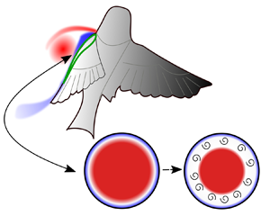
Figure 1. (a) Sketch of an LEV on a bird's wing with an arrow pointing to the position of the vorticity-annihilating boundary layer. (b) Vorticity evolution (colour coded) and (c) the azimuthal velocity profile ( $\left \langle {u_{\varphi }} \right \rangle$) in stages I to III of the spin-down: initial condition (i.c.); laminar stage (I); instabilities and transition to turbulence (II); and sustained turbulence with intact vortex core and a region of constant angular momentum (III).
In the current study, the interaction of a vortex with a wall is abstracted to the canonical flow of a decaying vortex from solid-body rotation (SBR), which in the following is referred to as the spin-down process; see figure 1(b). The vortex in SBR (angular velocity  $\varOmega$) is placed inside an impulsively stopped cylinder of radius $R$ with a cylindrical coordinate system ( $r,\varphi ,z$) placed at its centre. For a fluid of viscosity $\nu$ the temporal evolution of the spin-down process from the initial conditions,
 \begin{equation} u_\varphi(r) = \varOmega r, \quad u_r = u_z = 0, \end{equation}
depends on the Reynolds number
 \begin{equation} Re=\frac{\varOmega R^{2}}{\nu} \end{equation}
and a dimensionless time
 \begin{equation} \theta = \nu t/R^{2}. \end{equation}
Alternatively, the external dimensionless time  $\varOmega t=\theta Re$ can be utilised, where $\varOmega t=2{\rm \pi}$ represents a full revolution of the SBR. For a limited range of $Re<2.8 \times 10^{4}$, Kaiser et al. (Reference Kaiser, Frohnapfel, Kriegseis, Ostilla-Monico, Rival and Gatti2020) identified five successive stages of the spin-down process. Figure 1(b) shows the evolution of vorticity during the early stages, while figure 1(c) presents the spatially averaged azimuthal velocity profile $\left \langle {u_\varphi } \right \rangle =\left \langle {u_\varphi } \right \rangle _{\varphi ,z}(r,t)$. After the formation of a laminar boundary layer (stage I) a primary centrifugal instability mechanism occurs and leads to the formation of streamwise laminar Taylor rolls that subsequently break down owing to secondary instabilities (stage II), initiating the transition to turbulence. During the turbulent stage III, the vortex core is still intact and in SBR. However, between the vortex core (blue in figure 1c) and a turbulent near-wall region (red), a turbulent region is established (purple) that – in spatial average – is vorticity-free ( $\left \langle {\omega _z} \right \rangle =0$). In this vorticity-free region the angular momentum $l(t)=\left \langle {u_{\varphi }} \right \rangle r$ is spatially constant and only a function of time ( $t$, see figure 1c). Eventually the vortex core breaks down (stage IV) and the flow relaminarises (stage V). Kaiser et al. (Reference Kaiser, Frohnapfel, Kriegseis, Ostilla-Monico, Rival and Gatti2020) define the boundary-layer thickness $\delta _{99}$ as the distance from the cylinder wall, where $\left \langle {u_{\varphi }} \right \rangle$ deviates $1\,\%$ from the initial condition; see figure 1(c). The magnitude of $\delta _{99}$ grows continuously during the spin-down until the vortex core breaks down and the complete cylinder contains a turbulent flow ( $\delta _{99}/R=1$).
The effects of curved streamlines, in combination with the oppositely signed vorticity layers, influences all stages starting from the centrifugal instability (Rayleigh Reference Rayleigh1917; Euteneuer Reference Euteneuer1972) over the turbulent statistics (Meroney & Bradshaw Reference Meroney and Bradshaw1975) to the decay of anisotropic turbulence (Ostilla-Mónico et al. Reference Ostilla-Mónico, Zhu, Spandan, Verzicco and Lohse2017). For increasing  $Re$, however, transition to turbulence occurs earlier (Kim & Choi Reference Kim and Choi2006), and therefore the ratio of the boundary-layer thickness ( $\delta _{99}$) to the integral length scale ( $R$), at which transition occurs, decreases ( $\delta _{99}/R\ll 1$). In the related Taylor–Couette problem, the impact of vanishing curvature effects ( $d/R\ll 1$, where $d$ is the gap between inner and outer cylinder) was extensively studied. The flow approaches either the linearly stable plane-Couette problem that usually undergoes a nonlinear instability (Faisst & Eckhardt Reference Faisst and Eckhardt2000) or the rotating plane-Couette flow (Nagata Reference Nagata1990; Nagata, Song & Wall Reference Nagata, Song and Wall2021). For the present spin-down problem, small values of $\delta _{99}/R\ll 1$ lead to a flow that approaches the acceleration of a flat plate relative to a fluid. This so-called Stokes’ first problem is linearly unstable and destabilises owing to Tollmien–Schlichting (TS)-like waves (Luchini & Bottaro Reference Luchini and Bottaro2001). Comparing the stability analyses for centrifugal instability and TS waves, respectively, the critical times $\theta _c$, at which transition is expected, can be retrieved (Luchini & Bottaro Reference Luchini and Bottaro2001; Kim & Choi Reference Kim and Choi2006). As discussed in Appendix A, the critical times scale with $\theta _c^{CI} \propto Re^{-4/3}$ in the case of centrifugal instability and with $\theta _c^{TS} \propto Re^{-2}$ in the case of a TS instability. This is in agreement with the intuition that the TS instability eventually dominates at very large $Re$. As it yet remains unclear whether the centrifugal instability dominates over the entire $Re$ range relevant for animal propulsion, the present study aims to close this gap in the literature.
Furthermore, in stage III and at moderate  $Re$, the region of constant angular momentum ( $\left \langle {\omega _z} \right \rangle =0$) can be explained in terms of curved streamlines (Rayleigh Reference Rayleigh1917). As streamline curvature is expected to be small during the onset of turbulence at high $Re$, the present study also explores whether and when a region of constant angular momentum is established in the investigated $Re$ range.
To assess how a very high  $Re$ influences vorticity annihilation for both the transition-to-turbulence (stage II) and the sustained-turbulence stage (stage III), spin-down experiments up to stage III of the spin-down process were performed for $Re \leq 4 \times 10^{6}$. The experiments explored in the current study increase the $Re$ range significantly in comparison with prior direct numerical simulations (DNS) in Kaiser et al. (Reference Kaiser, Frohnapfel, Kriegseis, Ostilla-Monico, Rival and Gatti2020) ( $Re\leq 2.8\times 10^{4}$) and experimental investigations by Euteneuer (Reference Euteneuer1972), and Mathis & Neitzel (Reference Mathis and Neitzel1985) ( $Re\leq 2.5 \times 10^{4}$). This large advancement in $Re$ becomes possible through the unique combination of a large-scale facility with a novel approach to reduce end-wall effects.
2. Experimental methods
To systematically expand the  $Re$ range from data available in the literature ( ${Re\leq 2.8 \times 10^{4}}$) up to very high $Re$ ( $Re\leq 4 \times 10^{6}$), two experimental campaigns with complementary length scales were performed; see figure 2. A small-scale experiment (SSE; $2R=0.49\ \textrm {m}$, $2.8 \times 10^{4}\leq Re \leq 5.6 \times 10^{5}$) at the Karlsruhe Institute of Technology and a large-scale experiment (LSE; $2R=13.00\ \textrm {m}$ and $5.2 \times 10^{5}< Re<4 \times 10^{6}$) at the CORIOLIS II platform in Grenoble were conducted. In both campaigns the cylindrical containers were filled with water (height $H$, kinematic viscosity $\nu$, density $\rho _w$). Duck & Foster (Reference Duck and Foster2001) provide a comprehensive review of the effects of end-wall boundary layers on the flow in accelerated cylinders. As in the present study only the vorticity annihilation in the side-wall boundary layer is explored, end-wall effects are not of interest and should be minimised. To reduce end-wall effects, the experiments were performed in an open-surface configuration. Furthermore, in some runs (both SSE and LSE) a saturated salt-water layer ( $\rho _s=1.2\ \mathrm {g}\,\mathrm {cm}^{-3}$) of height $H_s$ was placed under the measurement volume at the bottom of the respective cylindrical container. Appendix B provides a detailed description of the experimental design of the salt-water layer approach and a comparison with results without this additional layer. It is shown that the salt-water layer successfully mitigates end-wall effects as long as the interface between the salt-water layer and the fresh-water layer remains stable.

Figure 2. Set-up of the SSE (a) and the LSE (b). Stereo PIV system focused on the near-wall region (red), planar PIV system covering the long-term boundary-layer evolution (blue), and planar PIV to assess the coherence of the vortex core (orange). Filling height  $H$, axial position of the measurement plane $H_m$ and height of the saturated salt-water layer $H_s$.
The spin-down process was captured by means of planar and stereoscopic particle image velocimetry (PIV). Therefore, a horizontal laser light sheet was introduced for both campaigns (SSE and LSE) at height  $H_m=0.5H$ and the water was seeded with polyamide 12 particles. Further details of the respective set-ups and experimental parameters are outlined in the following.
2.1. Small-scale experiments
As depicted in figure 2(a) an acrylic glass cylinder with an inner diameter of  ${2R=0.49\ \mathrm {m}}$ was filled with distilled water ( $\rho _w=997\ \mathrm {kg}\,\mathrm {m}^{-3}$) and mounted to an aluminium framework via ball bearings that allow co-axial rotation of the cylinder. The cylinder was propelled by a closed-loop controlled step motor that allowed for fast deceleration without an additional braking device. Spin-down experiments in the range of ${0.47\,\mathrm {s}^{-1}\leq \varOmega =2{\rm \pi} f \leq 9.42\,\mathrm {s}^{-1}}$ were performed, which corresponds to the aforementioned $Re$ range of $2.8 \times 10^{4}< Re<5.6 \times 10^{5}$. For all angular velocities ( $\varOmega$) tested, the cylinder decelerated to rest within less than one revolution.
A low-speed planar PIV system consisting of a double-frame CCD camera (PCO Pixelfly,  $1392\ \textrm {px} \times 1040\ \textrm {px}$, lens: Nikon AF Nikkor $50\ \textrm {mm}$ $f/1.4D$) and a dual-pulsed Nd:YAG laser (Quantel Evergreen 70) was utilised to provide double-frame images at 5 Hz, leading to a delay of $\Delta t=0.2\ \textrm {s}$ between two consecutive velocity fields. The field of view (FOV) in the image plane resulted in $110\ \textrm {mm}$ $\times$ $82\ \textrm {mm}$ with a resolution of $12.7\ \textrm {px}\,\textrm {mm}^{-1}$. The pulse distance was adapted to the initial condition (i.e. $\varOmega$) of the respective experiments to ensure a maximum displacement of 15 px. Tests at different aspect ratios ( $A$)
$A$)  $0.5\leq A=H/R \leq 2.0$ were performed to examine the influence of $A$ on the end-wall effects.
2.2. Large-scale experiments
The CORIOLIS II platform was filled up to  $H=1\ \textrm {m}$ with a weak saline solution ( $\rho _w= 1004\ \mathrm {kg}\,\mathrm {m}^{-3}$) resulting in $A=2/13$. The slightly higher density of the saline solution compared to the distilled water used in the SSE decreased the density difference between water and polyamide 12 particles ( $\rho _p=1014\ \mathrm {kg}\,\mathrm {m}^{-3}$) and thereby minimised settling of the particles during the extended spin-up times to SBR of 3 h before the start of the spin-downs. Experiments at various revolution times of the initial SBR within the range $120\ \mathrm {s} \leq 1/f \leq 470\ \textrm {s}$ were performed, resulting in a $Re$ range of $0.5 \times 10^{6} \leq Re \leq 4.0 \times 10^{6}$ for the LSE. Figure 2(b) provides an overview of the three PIV setups that were operated simultaneously. All three PIV set-ups utilised the same horizontal laser light sheet produced by a continuous 25 W Spectra Physics Millennia laser. A stereo set-up (red) took advantage of the optical access through the same window as the light sheet. Two Phantom Miro M310 cameras (Nikon AF Micro-Nikkor $60\ \textrm {mm}$ $f/2.8D$) were used to record the near-wall region with a resolution of $14.5\ \textrm {px}\,\textrm {mm}^{-1}$. The long-term evolution of the boundary layer was recorded with a planar, time-resolved three-camera system consisting of two pco.edge 5.5 cameras (lens: Samyang ED AS UMC $35\ \textrm {mm}$) and a Dalsa Falcon 4M camera (lens: Nikon AF Nikkor $28\ \textrm {mm}$ $f/2.8D$). The combined FOV had a radial extent of approximately $75\ \mathrm {cm}$ and a resolution of $10\ \textrm {px}\,\textrm {mm}^{-1}$. The frame rate of the time-resolved measurements was set to achieve a maximum particle displacement of 30 px between two consecutive images. The frame rates varied within the range of 25–400 Hz ( $0.0025\ \mathrm {s} \leq \Delta t \leq 0.04\ \textrm {s}$) dependent on $Re$ and the FOV of the planar and the stereo set-up, respectively. Finally, a pco.1200 HS camera (lens: Nikon AF Nikkor $50\ \textrm {mm}$ $f/1.4D$; orange in figure 2b) was used to record the coherence of the vortex core at an approximate side-wall distance of $1.5\ \textrm {m}$ ( $R_{hs}=5\ \textrm {m}$). A FOV of $25\ \mathrm {cm} \times 20\ \mathrm {cm}$ resulted in a resolution of approximately $5\ \textrm {px}\,\textrm {mm}^{-1}$.
3. Results
The present section discusses the  $Re$ scaling of the vorticity-annihilating boundary layer. In particular, the onset of laminar-to-turbulent transition (§ 3.1) and the turbulent boundary-layer growth (§ 3.2) are investigated. Finally, the findings on the scaling of the transition to turbulence and the scaling of the turbulent boundary-layer growth are combined to examine the $Re$ scaling of vorticity annihilation (§ 3.3).
3.1. Transition
Two aspects of the transition  $Re$ scaling are observed in the present section. First, it is to be validated if at very high $Re$ centrifugal instabilities are still the primary instability mechanism yielding transition to turbulence in the boundary layer. Second, the time instance $\theta _o=\nu t_o/R^{2}$, where $\left \langle {u_{\varphi }} \right \rangle$ first deviates from a stable laminar profile, is captured and compared with analytical, numerical, and experimental studies at smaller $Re$, as reported in the literature.
As mentioned in § 1, a higher  $Re$ causes an earlier onset of the primary instability and therefore a thinner boundary layer ( $\delta _{99}$) when the instability occurs. Therefore, diminishing curvature effects ( $\delta _{99}/R\ll 1$) are expected and the boundary layer asymptotically approaches Stokes’ first problem, which is a boundary layer with TS-like waves rather than Taylor rolls as its primary instability. To identify which instability mechanism dominates at high $Re$, the vorticity distribution is assessed by means of the highly resolved stereo PIV data. In case the centrifugal instability occurs first, characteristic plumes evolve from the wall that lead to rapidly growing laminar Taylor rolls as sketched in figure 3(a). Dependent on the relative position of the PIV laser sheet to the Taylor rolls, the footprint of the Taylor rolls in the captured data varies. In the centre of the plumes (case $i$, in figure 3a) slow fluid is transported from the near-wall region into the flow, while at the outer border of the plumes fast fluid is transported towards the wall (case $ii$). The most unique footprint of the Taylor rolls occurs in the plane where slow fluid engulfs the faster fluid (case $iii$). The resulting inflection points in the azimuthal velocity profile cause wall-parallel layers of axial vorticity $\omega _z$ with opposite signs in the PIV data; see figure 3(b). The relative position of the laser sheet and the Taylor rolls varies from experiment to experiment, and even within a single run as the Taylor rolls grow in size and/or are not perfectly axisymmetric. In approximately $90\,\%$ of the LSEs the characteristic footprint of laminar Taylor rolls (case $iii$) was detected in the PIV data during transition. Thus, it can be concluded that the centrifugal instability dominates even for the very weak streamline curvature in the present $Re$ range.

Figure 3. (a) Sketch of the  $\omega _z$ distribution in the streamwise vortices; (b) footprint of streamwise vortices in the PIV measurements during a spin-down at ${Re=1\times 10^{6}}$; and (c) onset of the centrifugal instability. Comparison of SSE and LSE with numerical data (empty markers), prior experiments (filled markers) and stability theory (lines). For ${Re\geq 2\times 10^{6}}$ (data to the right of the dotted line), the CORIOLIS II platform was not fully at rest at the onset of the instability. The data contained in (c) are also provided in Appendix A.
After the presence of Taylor rolls is confirmed, their onset time ( ${\theta _o=\nu t_o/R^{2}}$) can be compared with prior experiments of smaller $Re$ and predictions from stability analysis. We define the time instant $\theta _o$ as the time where the mean velocity profile ( $\left \langle {u_{\varphi }} \right \rangle$) first deviates from the analytical stable laminar solution given by Neitzel (Reference Neitzel1982). The large scales of the LSE facility ( $R=6.5\ \textrm {m}$), in combination with the time-resolved measurements ( $25-400$ frames per second, dependent on $Re$ and PIV set-up), lead to a high temporal resolution in normalised units ( $\theta =\nu t/R^{2}$) and thereby allow for an accurate estimate of $\theta _o$. The supplementary movies (movie 1 and movie 2) available at https://doi.org/10.1017/jfm.2021.600, show the process to determine $\theta _0$ for two experiments at $Re\approx 1\times 10^{6}$ and $Re\approx 2.6\times 10^{6}$, respectively. In movie 1 case $ii$ occurs first, resulting in a temporally decreasing $\delta _{99}$ before case $iii$ is detected. Eventually, the secondary instability initiates the transition to turbulence. In movie 2 only case $iii$ is observed. Note that owing to the very high $Re$ in movie 2, the centrifugal instability emerged before the CORIOLIS II platform was completely at rest. Therefore, the azimuthal velocity ( $\left \langle {u_{\varphi }} \right \rangle$) was normalised by $\Delta \varOmega (t) R$, where $\Delta \varOmega (t)$ is the instantaneous change of the platform's angular velocity and $\Delta \varOmega =\varOmega$ once the platform is as rest.
Figure 3(c) shows a comparison between the present results with the onset times of prior SSE, numerical simulations, and stability theory. Kim & Choi (Reference Kim and Choi2006) utilised propagation theory to determine the scaling of the critical time  $\theta _c=\nu t_c/R^{2}=9.4 Re^{-4/3}$ at which the linear instability first grows at a faster rate than the mean flow decays. Comparing critical and onset times, Kim & Choi (Reference Kim and Choi2006) observed that $\theta _o \approx 4 \theta _c$. While the present data exceeds the $Re$ range of prior measurements by two orders of magnitude, the experimental results still follow the predicted scaling.
Only for  $Re\geq 2\times 10^{6}$ (right of the dotted line in figure 3c) do the data deviate from the expected behaviour. The deviation can be explained by the significant deceleration times of the CORIOLIS II platform. Owing to its high mass, the platform cannot be stopped instantly. Therefore, even though the platform was decelerated at the fastest possible rate, it was not fully at rest when instabilities occurred for the highest $Re$ experiments.
3.2. Turbulent boundary-layer growth
After the transition to turbulence, stage III of the vortex decay begins. For small  $Re$, the flow during stage III can be partitioned into three regions (see figure 1c): a core in SBR, a turbulent region of, in spatial average, constant angular momentum $l(t)=\left \langle {u_{\varphi }} \right \rangle (t)r$ (equivalent to $\left \langle {\omega _z} \right \rangle =0$), and a turbulent shear layer near the wall. As a result, the region of constant angular momentum represents the marginal case of the Rayleigh criterion (Rayleigh Reference Rayleigh1917). As such, the region of constant angular momentum only exists owing to the curved streamlines of the mean flow. Furthermore, Kaiser et al. (Reference Kaiser, Frohnapfel, Kriegseis, Ostilla-Monico, Rival and Gatti2020) observed that $\delta _{99}$ grows at the same rate ( $\sim \sqrt {\nu t}$) during stage III ( $\delta ^{III}_{99}$) as for the laminar stage (stage I, $\delta ^{I}_{99}$); however, with different coefficients, $a_{turb}(Re)$ and $a_{lam}$, respectively,
 \begin{equation} \delta_{99}^{I}=a_{lam}\sqrt{\nu t}, \quad \delta_{99}^{III}=a_{turb}(Re)\sqrt{\nu t}, \end{equation}
where  $a_{lam} \approx 3.68$ for all $Re$. For the limited range $3\times 10^{3}< Re<2.8 \times 10^{4}$, Kaiser et al. (Reference Kaiser, Frohnapfel, Kriegseis, Ostilla-Monico, Rival and Gatti2020) suggested the empirical scaling law
 \begin{equation} a_{turb}=0.1 Re^{1/3} a_{lam}. \end{equation}
 The present section expands on whether (a) the region of constant angular momentum, and (b) the scaling given by (3.2) prevail for high  $Re$.
$Re$.
To identify if the region of constant angular momentum also exists for large  $Re$, a robust estimate of the mean azimuthal velocity profile ( $\left \langle {u_{\varphi }} \right \rangle =\left \langle {u_{\varphi }} \right \rangle _{\varphi ,z}(r,t$)) is needed. Figure 4 shows PIV data for five time instances throughout the laminar, transitional and turbulent stages for $Re=2.6\times 10^{6}$. To obtain a good approximation of the mean velocity profile ( $\left \langle {u_{\varphi }} \right \rangle$), the data are averaged along the $\varphi$-direction over the azimuthal extent of the PIV–FOV ( $\left \langle {u_{\varphi }} \right \rangle _\varphi$, red lines). During the laminar stage, the azimuthal velocity profile only depends on $r$ and thus $u_{\varphi }=\left \langle {u_{\varphi }} \right \rangle =\left \langle {u_{\varphi }} \right \rangle _\varphi$ for $t< t_o$ (see inlay in figure 4). However, as only a small subset of the flow is captured via the PIV measurements, the spatial average over the FOV does not suffice to provide a converged estimate of the mean velocity once transition to turbulence begins ( $\left \langle {u_{\varphi }} \right \rangle _\varphi \neq \left \langle {u_{\varphi }} \right \rangle$ for $t>t_o$). To further smooth the data during the transitional and the turbulent stage, a moving time average ( $\left \langle {u_{\varphi }} \right \rangle _{\varphi ,t}$, black lines) over a small window $t_{avg}$ is calculated as follows:
 \begin{equation} \left\langle {u_{\varphi}} \right \rangle_{\varphi,t}(r,t)= \frac{1}{(\varphi_{max}-\varphi_{min})t_{avg}}\int_{\varphi=\varphi_{min}}^{\varphi_{max}} \int_{t^{*}=t-t_{avg}/2}^{t+t_{avg}/2}u_{\varphi}(r,\varphi,t^{*}) \,\mathrm{d}t^{*}\,\mathrm{d}\varphi, \end{equation}
where  $\varphi _{min}$ and $\varphi _{max}$ are the limits of the FOV. For the LSE, $t_{avg}$ was set to $2.5\,\%$ of the revolution time ( $t_{avg}=0.025/f$). In the case of the SSE, the data from three subsequent time steps of the low-speed PIV system (5 Hz) were averaged ( $t_{avg}=0.6\ \textrm {s}$).

Figure 4. Fitting techniques for a robust approximation of  $\delta _{99}$ are exemplarily shown for an experiment at ${Re\approx 2.6 \times 10^{6}}$ with a salt-water layer at five arbitrary time instances ${\varOmega t \in \{ 1.1,2.2,4.3,8.7,23.9 \}}$ corresponding to ${\theta =\nu t/R^{2} \in \{ 4.1,8.2,16.4,32.9,90.0 \}}\times 10^{-7}$. The applied fitting functions are: analytical solution of the laminar profile during laminar stage (also shown in inlay); linear fit during transition to turbulence; and a potential vortex during the turbulent stage. The three-camera-FOV of the planar-PIV measurements is shown highlighted in light green.
After the slow boundary-layer growth during stage I ( $\varOmega t=1.1$ in figure 4) the boundary layer grows rapidly once the flow destabilises (stage II). Eventually, once $\delta _{99}/R={O}(10^{-1})$, a region of constant angular momentum is established ( $\varOmega t=8.7$ in figure 4). Thus, independent of $Re$, the ratio $\delta _{99}/R$ is large enough that curvature effects cause the region of constant angular momentum and thereby indicate the onset of stage III. As such, the same consecutive stages of vortex decay (stages I–III) are expected for all $Re$.
$Re$.
In the following, the empirical scaling laws for  $\delta _{99}(t)$ ((3.1a,b), (3.2)) are tested for the present high $Re$. As $\delta _{99}$ is susceptible to measurement noise, further post-processing steps are applied in order to calculate an accurate estimate of $\delta _{99}$. Figure 4 presents the fitting functions (blue lines) that are applied to $\left \langle {u_{\varphi }} \right \rangle _{\varphi ,t}$ (black lines). For the laminar stage, the highly resolved stereo PIV data are fitted with the analytical solution of Neitzel (Reference Neitzel1982) as shown in the inlay of figure 4 (see also movie 1 and movie 2). During the transition to turbulence (stage II), $\delta _{99}$ quickly exceeds the FOV of the stereo-PIV system, which only recorded the near-wall region (see figure 2b). Therefore, the data of the planar three-camera system are utilised. In stage II, a linear fit is applied in the boundary layer (plus-shaped markers). For stage III, $l(t)/R$ is selected as the fitting function (triangular markers). For all stages, the intersection of the fit with the SBR (yellow markers in figure 4) is used to obtain an estimate for $\delta _{99}$. Note that this approach provides the possibility to estimate $\delta _{99}$ even beyond the FOV of the PIV measurements as exemplarily shown for $\left \langle {u_{\varphi }} \right \rangle _\varphi (r,\varOmega t=23.9)$ in figure 4.
Figure 5(a) shows a comparison of the evolution of  $\delta _{99}$ in the SSE and the LSE with the numerical data of Kaiser et al. (Reference Kaiser, Frohnapfel, Kriegseis, Ostilla-Monico, Rival and Gatti2020). The low-speed PIV system of the SSE only allowed us to track the complete transition process for the smaller $Re$; for larger $Re$, the normalised temporal resolution ( $\Delta \theta =\nu \Delta t/R^{2}$) of the SSE is insufficient. In contrast, time-resolved measurements and a large radius ( $R$) during the LSE allowed tracking of $\delta _{99}$ during the laminar and the transitional stage despite the high $Re$. Owing to the finite spin-down times of the large-scale facility used for the LSE, $\delta _{99}$ grows slightly slower during the laminar stage, as compared to an impulsively stopped cylinder (dotted black vs solid orange and blue lines in figure 5a).

Figure 5. (a) Boundary-layer growth  $\delta _{99}$ at various $Re$. The plotted curves correspond to $Re \in \{0.3, 0.6, 1.2, 2.8\}\times 10^{4}$ (DNS, Kaiser et al. Reference Kaiser, Frohnapfel, Kriegseis, Ostilla-Monico, Rival and Gatti2020), $Re \in \{2.8,5.6\}\times 10^{4}$ (SSE, salt, $A=0.5$), $Re \in \{2.8,5.6\}\times 10^{5}$ (SSE, no salt, $A=2.0$), and $Re \in \{2.0,2.7\}\times 10^{6}$ (LSE, salt, $A=2/13$). Dashed lines show the suggested empirical $Re$ scaling of turbulent boundary layers (3.2); and (b) $Re$ scaling of $a_{turb}/a_{lam}$.
As discussed in § 3.1, the onset of transition scales with  $Re$, which leads to small values of $\delta _{99}/R$ at the onset of the centrifugal instability. Once the centrifugal instabilities set in, the boundary layer grows rapidly during stage II for all $Re$ until the region of constant angular momentum is established and stage III (fully turbulent boundary layer with intact vortex core) begins.
As previously observed for the lower  $Re$ DNS data (Kaiser et al. Reference Kaiser, Frohnapfel, Kriegseis, Ostilla-Monico, Rival and Gatti2020), $\delta _{99}$ grows again proportionally to $\sqrt {\nu t}$ during stage III for all $Re$, with a $Re$-dependent proportionality factor $a_{turb}(Re)$. Figure 5(b) shows a comparison between the present experiments and the empirical scaling law given in (3.2) and shows good agreement for the largely extended $Re$ range. Therefore, the flow properties of this particular growth rate of the turbulent boundary layer, combined with the existence of a turbulent-flow region with constant angular momentum, appears characteristic of the spin-down over a wide range of $Re$.
$Re$.
From a turbulence-modelling point of view, the observed similarity between turbulent and laminar boundary-layer growth rate suggests the use of an eddy-viscosity approach. Introducing an effective eddy viscosity  $\overline {\nu _t}$, which is constant across the boundary layer and constant over time during stage III, yields
 \begin{equation} \delta_{99}^{III}=a_{lam}\sqrt{(\nu + \overline{\nu_t}) t} = \underbrace{ a_{lam}\sqrt{1 + \frac{\overline{\nu_t}}{\nu}}}_{a_{turb}} \sqrt{\nu t}. \end{equation}
The Reynolds-number dependency of  $a_{turb}$ is thus fully contained in $\overline {\nu _t}$. The overbar for $\overline {\nu _t}$ is chosen to indicate the surprising fact that the present data suggest the presence of an effective eddy viscosity that remains constant in a statistically unsteady turbulent flow.
While the experimental data do not provide the possibility of a deeper analysis, the lower- $Re$ DNS data of Kaiser et al. (Reference Kaiser, Frohnapfel, Kriegseis, Ostilla-Monico, Rival and Gatti2020) do provide some additional insight, which is summarised in Appendix C. It is found that the observed $Re$ scaling of $a_{turb}/a_{lam}$ can be recovered if one assumes a near-wall plateau of the turbulent Reynolds number, located underneath the region of constant angular momentum, to be the driving force behind $\overline {\nu _t}$.
3.3. Scaling of vorticity annihilation
After scaling laws for the onset of transition (§ 3.1) and the turbulent stage (§ 3.2) are established, the  $Re$ scaling of vorticity annihilation can be discussed. According to Morton (Reference Morton1984) vorticity is only introduced at a wall, when the wall is either accelerated or a streamwise pressure gradient exists. For the spin-down, no more vorticity is introduced when the cylinder is at rest, as no streamwise pressure gradient exists. Assuming an instantaneous deceleration, at $t=0$ all negative vorticity is in an infinitesimally small layer at the wall. As such, the cylinder circulation, written
 \begin{equation} \varGamma=\int_A \omega_z \mathrm{d}A = 2{\rm \pi} \int_{r=0}^{R} \left\langle {\omega_z} \right \rangle r \,\mathrm{d}r = 0, \end{equation}
is zero after the cylinder walls are impulsively stopped. During spin-down, the negative vorticity propagates into the core until eventually  $\left \langle {\omega _z} \right \rangle =0$ for all $r$ when the flow is at rest. This implies that there is a temporally decreasing amount of circulation $\varGamma _c$ in the core of the cylinder:
 \begin{equation} \varGamma_{c}=2{\rm \pi} \int_{r=0}^{R-\delta_{99}} \left\langle {\omega_z} \right \rangle r\,\mathrm{d}r. \end{equation}
The core circulation can further be approximated to be
 \begin{equation} \varGamma_c\approx 2 \varOmega {\rm \pi}(R-\delta_{99})^{2} \end{equation}
as  $\left \langle {\omega _z} \right \rangle =2\varOmega$ is constant in the vortex core while the vortex core is still intact (stages I–III). Combining (3.7) with (3.2) and (3.1a,b) allows us to reconstruct the decay of $\varGamma _c$ during stages I and III for a given $Re$.
$Re$.
In the following, the temporal evolution of vorticity annihilation is captured by comparing the evolution of  $\varGamma _c$ for various $Re$. Figure 6 presents the decay of the core circulation for $3\times 10^{3} \leq Re \leq 2.7 \times 10^{6}$. As $\varGamma _c$ can be approximated as a function of $\delta _{99}$ (see (3.7)), the stages of the boundary-layer growth shown in figure 5 are also visible in the evolution of $\varGamma _c$. During the laminar stage, $\varGamma _c$ decays slowly, before the transition to turbulence increases the decay rate. Eventually, once stage III is entered, the decay rate of $\varGamma _c$ decreases again. In viscous units ( $\theta$), the earlier onset of transition leads to a faster decay of $\varGamma _c$ with increasing $Re$ (figure 6a).

Figure 6. Vortex core circulation ( $\varGamma _c$) for various $Re$. The plotted curves correspond to $Re \in \{0.3, 0.6, 1.2, 2.8\}\times 10^{4}$ (DNS, Kaiser et al. Reference Kaiser, Frohnapfel, Kriegseis, Ostilla-Monico, Rival and Gatti2020), $Re \in \{2.8,5.6\}\times 10^{4}$ (SSE, with salt-water layer, $A=0.5$), $Re \in \{2.8,5.6\}\times 10^{5}$ (SSE, no salt-water layer, $A=2.0$), and $Re \in \{2.0,2.7\}\times 10^{6}$ (LSE, salt-water layer, $A=2/13$). (a) Time normalised in viscous units ( $\theta =\nu t/R^{2}$); and (b) time normalised in outer units ( $\varOmega t$).
Considering vortex–wall interactions on accelerated propulsors (wings or flippers, see § 1), the outer time scale  $\varOmega t$ provides a better comparison of the $Re$ scaling of vorticity annihilation. Observations in nature show that similar propulsors perform similar kinematics over a wide range of $Re$ (Taylor, Nudds & Thomas Reference Taylor, Nudds and Thomas2003; Gazzola et al. Reference Gazzola, Argentina and Mahadevan2014). As such, a relevant metric for comparing the $Re$ scaling would be how much vorticity is annihilated on the time scale of the kinematics, e.g. after a full revolution of the vortex on the propulsor ( $\varOmega t=2{\rm \pi}$). Figure 6(b) compares the decay of $\varGamma _c$ on an outer time scale ( $\varOmega t$). In this scaling, a smaller $Re$ leads to a faster decay of $\varGamma _c$ owing to more pronounced viscous effects during the laminar stage. However, this is (in part) compensated by earlier transition for high $Re$. As such, around a full revolution of the SBR ( $\varOmega t=2{\rm \pi}$, highlighted in figure 6b) multiple lines intersect, suggesting similar $\varGamma _c$ despite significantly different $Re$. The similar amount of annihilated vorticity (similar $\varGamma _c$) after one core revolution ( $\varOmega t=2{\rm \pi}$) could explain why similar kinematics are observed during vortex formation in animal locomotion for a wide range of $Re$. Typically, the formed vortices are shed from the respective propulsor after each stroke. Therefore, the vorticity-annihilating boundary prevails only for a finite time before the stroke ends. Note, however, that if the boundary-layer evolution takes place over an extended period of time ( $\varOmega t>20$), for instance by stabilising a LEV on a propulsor, a $Re$ scaling of the vorticity-annihilation process is likely to become more apparent, as shown in figure 6(b).
4. Concluding remarks
The interaction of vortices with solid boundaries leads to the formation of a unique boundary layer, where layers of oppositely signed vorticity interact. Two complementary experimental campaigns are presented that explore the  $Re$ scaling of an unsteady vorticity-annihilating boundary layer. The interaction of the vorticity from the vortex with the vorticity introduced at the wall is investigated in the canonical flow of a decaying SBR through a rapidly stopped cylinder. Experiments in a small ( $2R=0.49\ \textrm {m}$) and a large ( $2R=13.00\ \textrm {m}$) water-filled cylinder were conducted and captured by means of PIV. As only the side-wall boundary layer was of interest, the influence of the end walls in the experiments was reduced by introducing a layer of saturated salt-water at the bottom of the cylinders.
Thanks to this novel experimental approach, the scales of the present study ( $Re\leq 4\times 10^{6}$) exceed the $Re$ range in the literature by more than two orders of magnitude. The centrifugal instability was shown to persist as the dominant primary instability mechanism over the entire Reynolds-number range relevant for animal propulsion.
The scaling of the onset time ( $\theta _o$) of the primary instability is compared to the literature, and scales as expected ( $\theta _o\propto Re^{-4/3}$). After transition to turbulence a turbulent flow region of constant angular momentum is established. The thickness of the subjacent boundary layer grows proportionally to $\sqrt {\nu t}$ for all investigated $Re$ such that ${\delta _{99}=a_{turb}(Re)\sqrt {\nu t}}$. The proportionality constant $a_{turb}$ is $Re$ dependent and the empirical scaling law ${a_{turb}/a_{lam} = 0.1\times Re^{1/3}}$, that was suggested based on previous DNS studies at smaller $Re$ by Kaiser et al. (Reference Kaiser, Frohnapfel, Kriegseis, Ostilla-Monico, Rival and Gatti2020), is validated for very high $Re$. Based on the DNS data it is shown that this scaling law can be recovered under the assumption that a near-wall plateau of the turbulent Reynolds number, which is constant in time during stage III of this statistically unsteady turbulent flow, governs the turbulent boundary-layer growth through an effective eddy-viscosity approach.
Finally, the observed findings and derived insights from the reported canonical case are elaborated in terms of the transferability from decaying SBR in a rapidly stopped cylinder, to applications of unsteady vortex formation such as LEVs. The centrifugal instabilities during LEV formation reported by Buchner et al. (Reference Buchner, Honnery and Soria2017) could only be shown at medium  $Re={O}(10^{4})$ and it yet remained unclear if at higher $Re$ the centrifugal instability mechanism would prevail and/or have a significant impact on the flow. In the present study, we find that Taylor rolls can also be expected during vortex formation at very high $Re$. Furthermore, the effect of the centrifugal instability on the vorticity annihilation process is significant throughout all $Re$. During the transition to turbulence (triggered by the centrifugal instability), the boundary layer grows rapidly until ${\delta _{99}/R={O}(10^{-1})}$. Thereby, significant amounts of vorticity are annihilated and eventually a region of constant angular momentum ( $\langle \omega _z \rangle =0$) is formed.
The empirical scaling law for the boundary-layer growth rate (3.2) allows us to estimate how quickly the vorticity in the boundary layer cross-annihilates. To quantify the temporal evolution of vorticity annihilation, the decay of the remaining circulation in the vortex core ( $\varGamma _c\approx 2\varOmega {\rm \pi}(R-\delta _{99})^{2}$; (3.7)) is monitored on both a viscous as well as on an outer time scale for a wide range of $Re$. For higher $Re$ the effects of viscosity are smaller and thus the viscous diffusion of oppositely signed vorticity from the laminar boundary layer to the fluid core in SBR is significantly slower. However, the earlier onset of transition ( $\theta _o$) and the rapid vorticity annihilation taking place during the transition to turbulence partially compensate for the reduced effects of viscosity. As such, the amount of annihilated vorticity after one revolution of the vortex core is similar for a wide range of $Re$ (see § 3.3). This similarity in the vorticity-annihilation rate during the early stages could partially explain the similar propulsor kinematics observed in nature across a wide range of scales (Taylor et al. Reference Taylor, Nudds and Thomas2003; Gazzola et al. Reference Gazzola, Argentina and Mahadevan2014). The vortices formed in nature often detach from the propulsor after a few revolutions (end of the stroke), leading to a similar contribution of vorticity annihilation to the circulation budget of the LEV, independent of $Re$. Future work could address the $Re$-scaling effects of permanently stabilised LEVs as for example investigated by Lentink & Dickinson (Reference Lentink and Dickinson2009). It is hypothesised that once the dynamics of the laminar-to-turbulent transition are excluded, $Re$ will have a more significant influence on the circulation budget of the LEV.
Supplementary movies
Supplementary movies are available at https://doi.org/10.1017/jfm.2021.600.
Acknowledgements
The authors would like to thank S. Jakirlić for helpful discussions on the eddy-viscosity concept, which was suggested be introduced by one of the anonymous reviewers.
Funding
This work is supported by the Priority Programme SPP 1881 Turbulent Superstructures of the Deutsche Forschungsgemeinschaft (DFG) and as project ANNI by the European High-Performance Infrastructures in Turbulence Consortium (EuHIT).
Declaration of interests
The authors report no conflict of interest.
Appendix A. Centrifugal instability and TS waves
A.1. Critical time  $\theta _c$

Before the onset of the instability the boundary layer grows as  $\delta _{99}=a_{lam}\sqrt {\nu t}$ (Kaiser et al. Reference Kaiser, Frohnapfel, Kriegseis, Ostilla-Monico, Rival and Gatti2020). At a critical time $\theta _c=\nu t_c/R^{2}$ a linear instability occurs. To estimate if, for a given $Re$, either the centrifugal instability ( $\theta _c^{CI}$, Kim & Choi Reference Kim and Choi2006) or TS waves ( $\theta _c^{TS}$, Luchini & Bottaro Reference Luchini and Bottaro2001) occur first, the present section compares $Re$ scaling of the respective problem based on linear instability analysis. The similarity to the Taylor–Couette problem suggests a Taylor number for the spin-down flow that for small $\delta _{99}$ simplifies to
 \begin{equation} Ta=\frac{\varOmega (R-\delta_{99})^{1/2}\delta_{99}^{3/2}}{\nu}\approx Re \left( \frac{\delta_{99}}{R} \right)^{3/2} =Re \left( \frac{a_{lam}\sqrt{\nu t}}{R} \right)^{3/2}, \end{equation}
where  $Re=\varOmega R^{2}/\nu$. Assuming the onset of transition at a critical time $t_c^{CI}$ and a critical Taylor number $Ta_c$, (A1) leads to
 \begin{equation} \theta_c^{CI}=\frac{\nu t^{Ta}_c}{R^{2}} = \frac{Ta_c^{4/3}}{a_{lam}^{2}}Re^{{-}4/3}=C_1 Re^{{-}4/3}. \end{equation}
Kim & Choi (Reference Kim and Choi2006) found the same scaling with a stability analysis. Based on the growth rate of the kinetic energy of the disturbance, Kim & Choi (Reference Kim and Choi2006) defined  $\theta ^{IC}_c$ and estimated $C_1=9.4$.
For very high  $Re$ and with vanishing curvature effects, the spin-down flow approaches Stokes’ first problem. A boundary-layer Reynolds number $Re_\delta$ can be approximated to
 \begin{equation} Re_\delta=\frac{U\delta_{99}}{\nu}=\frac{\varOmega (R-\delta_{99}) \delta_{99}}{\nu}\approx Re \left( \frac{\delta_{99}}{R} \right)=Re \left( \frac{a_{lam}\sqrt{\nu t}}{R} \right). \end{equation}
Equation (A3) provides the relation of a critical Reynolds number  $Re_\delta ^{c}$ and the critical time
 \begin{equation} \theta_c^{TS}=\frac{\nu t^{TS}_c}{R^{2}} = (Re_\delta^{c}/a_{lam})^{2} Re^{{-}2}\, = C_2 Re^{{-}2}. \end{equation}
For Stokes’ first problem Luchini & Bottaro (Reference Luchini and Bottaro2001) defined  $\theta _c^{TS}$ as the instance in time where disturbances of a critical wavelength first get amplified, leading to $C_2\approx 1485.68^{2}$.
It is apparent that  $\theta _c^{TS} \propto Re^{-2}$, while $\theta _c^{CI} \propto Re^{-4/3}$. As such, for very high $Re$ the TS waves should occur before the centrifugal instabilities. Note, however, that a quantitative comparison of the critical times based on (A2) and (A4) cannot be performed as Luchini & Bottaro (Reference Luchini and Bottaro2001) and Kim & Choi (Reference Kim and Choi2006) use deviating definitions of $\theta _c$. Furthermore, the remaining curvature of the spin-down problem, even at very high $Re$, might influence $\theta _c^{TS}$ and was neglected for the scaling estimates performed in this section.
A.2. Onset time $\theta _0$

The centrifugal instability dominates in the preset  $Re$ range and scales according to the predictions of Kim & Choi (Reference Kim and Choi2006). To allow for the validation of future numerical studies, the data of figure 3(c) are listed in table 1. As $Re$ not only depends on $\varOmega$ and $R$ but also on $\nu$, the temperature changes of the water in between different runs were monitored and explain the slight variations of $Re$ for LSE with the same initial conditions (i.e. $\varOmega$, $R$).
$R$).
Table 1. Onset of the centrifugal instability for the SSE and the LSE. The table contains the data of figure 3.

Appendix B. End-wall effects and their reduction
Duck & Foster (Reference Duck and Foster2001) provide a comprehensive review of the flow in angular-accelerated (enclosed) cylinders of height  $H$ with walls at the top and bottom. The end-wall boundary layer significantly influence all stages of the flow and thereby modifies the behaviour of the side-wall boundary layer. As such, end-wall effects are minimised in the present study. While in numerical investigations end walls can easily be removed by choosing periodic boundary conditions in the axial direction, a more elaborate solution was used for the present experimental implementations of the decaying SBR. Prior small-scale experimental campaigns by Euteneuer (Reference Euteneuer1972), Mathis & Neitzel (Reference Mathis and Neitzel1985) and Burin et al. (Reference Burin, Ji, Schartman, Cutler, Heitzenroeder, Liu, Morris and Raftopolous2006) successfully minimised the end-wall influence through either large-aspect-ratio cylinders ( $A=H/R$) or segmented end walls. However, both aforementioned methods come with high cost, when applied to large scales (large $R$). An alternative approach was suggested by Pedlosky (Reference Pedlosky1967), who used two layers of immiscible fluids with different densities. If the upper layer is confined by a free surface, linear theory predicts a significantly reduced contribution of end-wall effects on the upper layer. The experimental results of O'Donnell & Linden (Reference O'Donnell and Linden1992) on accelerating cylinders validated the theoretical predictions. As expensive and/or hazardous fluids cannot be used for LSEs, a saturated salt-water solution (density $\rho _S$) was chosen as the high-density fluid and fresh water was used for the upper layer. As the two fluids were then miscible, the stability of the interface, as well as the reduction of end-wall effects, were recorded in the SSE and the LSE via a GoPro camera focused on the interface between the two layers.
B.1. Interface stability of the saline-solution-water interface
O'Donnell & Linden (Reference O'Donnell and Linden1992) stated that if the interface between two stratified fluids interacts with the end wall during the spin-down process, the interface destabilises. To avoid end-wall-interface interaction, the minimum required height of the salt-water layer  $H_s^{min}$ was estimated analytically. The conservative (while non-physical) assumption of an instantaneous deceleration to rest of the salt-water layer during the spin-down process, while the top layer remains in SBR, leads to
 \begin{equation} H_s^{min}=\frac{\rho_w}{\rho_s-\rho_w} \frac{\varOmega^{2} R^{2}}{4g}. \end{equation}
For all experiments the height of the salt-water layer was chosen such that  $H_s>H_s^{min}$.
Furthermore, it is hypothesised that the interface stability during spin-down depends on the ratio between the kinetic energy that is dissipated during spin-down ( $\rho _s \varOmega ^{2} R^{2}$) and the stabilising effects of the potential energy $(\rho _s-\rho _w)gH_s$, where $H_s$ is the height of the salt-water layer. The ratio between the destabilising and the stabilising effects yields the interface Froude number
 \begin{equation} Fr_s=\frac{\rho_s \varOmega^{2} R^{2}}{(\rho_s-\rho_w) g H_s}, \end{equation}
where small values of  $Fr_s$ imply a stable interface. The critical Froude number $Fr_s^{c}$ at which the interface destabilises was determined in a series of SSE, before the LSE were designed. Table 2 provides an overview of the experiments that were performed. Despite the large differences in $Re$, the interface destabilised at similar $Fr_s^{c}$ for both the SSE and the LSE.
Table 2. Interface stability between the salt-water layer and the fresh-water layer. Reynolds number ( $Re$), Interface Froude number ( $Fr_{s}$), minimum salt-water level ( $H_s^{min}$) and the height of the salt-water level ( $H_s$).

B.2. Reduction of end-wall effects
The impact of the salt-water layer on the influence of end-wall effects was tested via PIV measurements.
Figure 7(a) shows the influence of  $A$ and the salt-water layer on the evolution of the azimuthal velocity profile for the SSE at $Re=5.6\times 10^{4}$. For $A=0.5$, and without the salt-water layer, the vortex core decays rapidly. A larger aspect ratio ( $A=2.0$) reduces the end-wall influence partially. However, introducing a salt-water layer proves to be even more efficient as the vortex core remains in SBR. For $Re=2.8 \times 10^{4}$ the experimental data show good agreement with the numerical results from Kaiser et al. (Reference Kaiser, Frohnapfel, Kriegseis, Ostilla-Monico, Rival and Gatti2020), as presented in figure 7(b) and thereby further validates the salt-water-layer approach.

Figure 7. Influence of ( $A$) and the presence of a salt-water layer on the flow characteristics during spin-down experiments. Five time instances ${\varOmega t \in \{ 2,8,16,32,64 \}}$ are presented. The SBR and regions of constant angular momentum $l(t)$ are emphasised using dotted and dashed lines, respectively. (a) $Re=5.6\times 10^{4}$ and (b) comparison of experimental results with DNS data from Kaiser et al. (Reference Kaiser, Frohnapfel, Kriegseis, Ostilla-Monico, Rival and Gatti2020) at $Re=2.8\times 10^{4}$.
For the LSE the core flow in SBR is captured by a single camera positioned at  $R_{hs}=5\ \textrm {m}$. The relative velocity of the fluid towards the platform ( $u^{rel}_\varphi$) is evaluated and spatially averaged over the complete FOV ( $\left \langle {u_{\varphi }} \right \rangle _{\varphi ,r}(t$)). Figure 8 presents $\left \langle {u_{\varphi }} \right \rangle _{\varphi ,r}(t)$ for various $Re$. As the CORIOLIS II platform requires a significant spin-down time owing to its large mass, for high $Re$, and without the salt-water layer, the influence from the bottom wall is found to be already present before the platform is completely at rest (see green line in figure 8a). In comparison, figure 8(b) clearly shows that the salt-water layer allows for a stable vortex core in SBR for large $\varOmega t<25$, approximately corresponding to four full revolutions of the vortex core ( $\varOmega t =8{\rm \pi}$).

Figure 8. End-wall effects and their reduction. While  $\langle u^{rel}_\varphi \rangle _{r,\varphi }/\varOmega R_{hs} \approx 1$, the core is still in SBR. The ramp of of the acceleration/deceleration process varies for different $Re$. The experiments where a saturated salt-water layer was introduced are marked with the tag ‘salt’.
Appendix C. Turbulent boundary-layer growth rate
The present experimental data reveal that the empirical scaling law for the turbulent boundary-layer growth rate suggested by Kaiser et al. (Reference Kaiser, Frohnapfel, Kriegseis, Ostilla-Monico, Rival and Gatti2020) based on DNS data in the Reynolds-number range  $3000 \leq Re \leq 28\,000$ is valid up to $Re=4 \times 10^{6}$. During stage III of the spin-down $\delta _{99}$ grows proportionally to $\sqrt {\nu t}$, i.e. similar to the laminar boundary layer, as described by (3.1a,b). The $Re$-dependent proportionality constant of the turbulent boundary-layer growth rate is related to the laminar growth rate by (3.2) throughout the entire investigated $Re$-range. This hints at a peculiar property of the turbulent boundary layer during stage III of the spin-down process.
As already noted by Kaiser et al. (Reference Kaiser, Frohnapfel, Kriegseis, Ostilla-Monico, Rival and Gatti2020) one interesting property of the turbulent boundary layer during this stage is the fact that the growth of  $\delta _{99}$ occurs simultaneous with a reduction of the friction velocity $u_\tau$ such that the friction Reynolds number $Re_{\tau }={u_\tau \delta _{99}}/{\nu }$ remains almost constant. In addition, the strong similarity of the turbulent boundary-layer growth rate with the laminar one enables a very simple modelling approach through a constant effective eddy viscosity $\overline {\nu _t}$ (3.4).
In the following, the DNS data of Kaiser et al. (Reference Kaiser, Frohnapfel, Kriegseis, Ostilla-Monico, Rival and Gatti2020) are used to explore this idea of  $\overline {\nu _t}$ further. In order to gain some insight into the effective viscosity ratio ${\overline {\nu _t}}/{\nu }$ we employ the turbulent Reynolds number $Re_t = {k^{2}}/{\nu \epsilon }$ (where $k$ and $\epsilon$ represent turbulent kinetic energy and viscous dissipation, respectively), which is related to the local viscosity ratio ${\nu _t}/{\nu }$ in the classical $k-\epsilon$ turbulence model through the model constant $C_{\mu }$ (Pope Reference Pope2000).
Figure 9(a) shows  $Re_t$ through stage III as a function of the wall distance in viscous units up to $\delta ^{+}_{99}=Re_\tau$.

Figure 9. The DNS data of Kaiser et al. (Reference Kaiser, Frohnapfel, Kriegseis, Ostilla-Monico, Rival and Gatti2020): (a) turbulent Reynolds number  $Re_t$ during stage III with a time-invariant near-wall plateau, which is described through its peak value $Re_{t,nw}$ at a time-invariant wall-normal location (vertical dotted lines); and (b) temporal evolution of $Re_{t,nw}$ during stages I–III. The dashed horizontal lines indicate proportionality to $Re^{2/3}$.
It can clearly be seen that for all investigated  $Re$ a near-wall plateau-like behaviour of $Re_t$ is present that remains almost constant over time, while far away from the wall (in the vorticity-free region) the peak of $Re_{t,out}$ increases.
Figure 9(b) presents the temporal evolution of the peak  $Re_t$ value within the near-wall plateau, referred to as $Re_{t,nw}$, in stages I-III. After an initial increase during transition, $Re_{t,nw}$ fluctuates around a constant value during stage III.
Interestingly,  $Re_{t,nw}$ appears to scale with $Re_{t,nw} \propto Re^{2/3}$ (dashed horizontal lines in figure 9), which recovers the observed $Re$ dependency of $a_{turb}(Re)$ under the assumptions that ${\overline {\nu _t}}/{\nu }\gg 1$ and ${\overline {\nu _t}}/{\nu } \propto Re_{t,nw}$, we can write
 \begin{equation} \frac{a_{turb}}{a_{lam}} \propto \sqrt{\frac{\overline{\nu_t}}{\nu}} \propto \sqrt{Re_{t,nw}} \propto Re^{1/3}. \end{equation}
The temporally invariant wall-normal location of  $Re_{t,nw}$ (visualised through the vertical dotted lines in figure 9a) is located within the buffer layer between the viscous sublayer and the region of logarithmic behaviour, and thereby outside of the region of constant angular momentum. The outer peak $Re_{t,out}$ is located in the centre of the constant angular momentum region.
The observation that the identified  $Re$ scaling of the turbulent boundary-layer growth can be recovered with $Re_{t,nw}$ hints at a physical relevance of this quantity for the turbulent boundary-layer growth rate under the spin-down conditions of stage III. This issue deserves further attention in future investigations.


 Open access