1. Introduction
The ice sheets have lost mass at an accelerating rate over the past decade, largely due to accelerated flow and drawdown at the margins. Several methods exist for observing surface elevation changes, including repeat laser and radar altimetry and stereoscopic digital elevation models (DEMs) from both airborne and satellite platforms (Reference Howat, Joughin and ScambosHowat and others, 2007; Reference Berthier and ToutinBerthier and Toutin, 2008; Reference Thomas, Frederick, Krabill, Manizade and MartinThomas and others, 2009). Each method has its advantages and disadvantages: imagery-based DEMs provide a continuous surface and therefore wide coverage in both space and time but have relatively large errors; laser altimeters, in contrast, have a high accuracy, but measurements are limited to the flight paths of the satellite or airplane, which in turn are limited by logistics and cost. As the largest surface changes in Greenland are observed at the ice margin, where surface slopes are high and the topography rough, neither of these datasets alone can be used to map the changes with both high spatial coverage and low errors. Such measurements are, however, important, as accurate estimates of elevation changes can be used to infer knowledge of changes in the mass balance and eustatic sea level (Reference SørensenSørensen and others, 2011).
The goal of this work is to make use of the complementary characteristics of stereoscopic DEMs and laser altimeter data to improve the spatial coverage and resolution of surface elevation and elevation change estimates. This is done for two Greenland outlet glaciers, Jakobshavn Isbræ (JI) and Kangerdlugssuaq (KL), for the period 2007–08. We develop a method in which the DEM surface is co-registered to altimeter data by fitting DEM observations to the altimeter point cloud using a least-squares adjustment, thereby minimizing planimetric and elevation-dependent errors and removing biases. We test multiple methods for geostatistically interpolating the residuals between the altimeter and co-registered DEM data to further adjust the final surface and provide confidence intervals for our estimates. This allows the production of corrected DEMs with a high spatial resolution even in areas of rough surface topography. Another important objective of this study is to examine how the confidence in surface elevation varies with distance from the altimeter flight paths, since this is essential information for planning future altimeter surveys. Several analyses have been conducted in which observations from the two sensors are combined: Reference Carabajal and HardingCarabajal and Harding (2005) used the Ice, Cloud and land Elevation Satellite (ICESat) to validate Shuttle Radar Topography Mission (STRM) C-band DEMs of the western United States by bilinear interpolation and comparison of the elevations, while Reference Korona, Berthier, Bernard, Rémy and ThouvenotKorona and others (2009) assumed ICESat data and SPOT 5 (Satellite Pour l’Observation de la Terre) DEMs from the SPIRIT (SPOT 5 stereoscopic survey of the Polar Ice: Reference Images and Topographies) campaign to be co-registered so the quality of the SPOT 5 observations could be tested. As such analyses can only provide reliable results if the co-registration works well, Reference Schenk, Csatho, Van der Veen, Brecher, Ahn and YoonSchenk and others (2005) developed a method in which knowledge of terrain features (e.g. ridge crests and sudden change of slope) and a least-squares approach could be used to shift a DEM in space in order to minimize the Euclidean distance to the altimeter point cloud. Reference Nuth and KääbNuth and Kääb (2011) developed a method similar to ours for glaciated areas, although they did not make use of the information lying in the elevation difference between the altimeter and DEM surfaces, which varies with the topography and changes in the observed area. We thereby take their method one step further by employing geostatistical spatial interpolation techniques.
2. Datasets
The DEMs are derived from SPOT 5 imagery obtained with the High Resolution Stereoscopic (HRS) sensor during the SPIRIT campaign (Reference Korona, Berthier, Bernard, Rémy and ThouvenotKorona and others, 2009). Due to the few repeat tracks from ICESat, these laser altimeter data are used in conjunction with lidar data from NASA’s Airborne Topographic Mapper (ATM) in order to ensure a high data coverage.
2.1. SPOT 5
The HRS sensor on board SPOT 5 is used to acquire stereoscopic pairs that can be combined to produce DEMs. Its two telescopes allow for along-track stereoscopy with a fore and aft view of 20° relative to nadir yielding a base-toheight (B/H) ratio of 0.8. The stereo pair consists of two images taken within a period of 90 s and covering an area of 600 km along-track × 120 km across-track. The short interval between the acquisition times ensures no significant temporal changes of the surface have occurred, while the use of a panchromatic band (0.48–0.7 m) minimizes the effects of shadows in areas of high relief. The resulting images have a pixel size of 5 m along-track × 10 m across-track with horizontal errors of 10–20 m, and elevation errors of 10–25 m depending on whether the surface is ice-covered or ice-free. The errors are caused, for example, by lack of radiometric contrasts in flat regions such as the snow-covered accumulation zone, steep slopes distorting the fore and aft view, or clouds moving and changing during the 90 s acquisition time. All of these break down the image correlation, thereby deteriorating the image quality (Reference Bouillon, Bernard, Gigord, Orsoni, Rudowski and BaudoinBouillon and others, 2006; Reference Berthier and ToutinBerthier and Toutin, 2008; Reference Korona, Berthier, Bernard, Rémy and ThouvenotKorona and others, 2009). Following the fourth International Polar Year (IPY), the French Space Agency (CNES), SPOT Image and LEGOS (Laboratoire d’Etudes en Géophysique et Océanographie Spatiales) initiated the SPIRIT campaign. The goal was to create an archive of HRS images over polar ice and for specific areas to produce DEMs with a spatial resolution of 40 m and elevation errors on the decimeter level. The SPIRIT product consisted of two DEMs (for gentle and steep slopes, respectively), two reliability masks showing the correlation score and identifying interpolated pixels, and an HRS orthoimage with a 5 m resolution. The imagery had an absolute horizontal accuracy of 30 m root-mean-square (RMS), and the campaign resulted in DEMs covering most major ice caps and outlet glaciers (Reference Korona, Berthier, Bernard, Rémy and ThouvenotKorona and others, 2009; Exelis Visual Information Solutions, 2011). The ones used here were acquired on 4 August 2007 and 2 August 2008 for JI and on 27 July 2007 and 21 September 2008 for KL. They were manually edited using ENVI in which cloud and rock masks were applied, and the datum was changed from the Earth Gravitational Model 1996 (EGM96) geoid to the World Geodetic System 1984 (WGS84) ellipsoid. The spatial structure of errors was not accounted for.
2.2. ICESat
The spaceborne laser measurements are conducted using the Geosciences Laser Altimeter System (GLAS) on board ICESat. When the emitted pulses intersect the surface, a circular spot with a diameter of ∼65 m is illuminated, and the along-track distance between two such consecutive footprints is 172 m. The data come from the GLAS/ICESat Antarctic and Greenland Ice Sheet Altimetry Data product (GLA12), release 31, and are downloaded from the US National Snow and Ice Data Center (NSIDC) website (Reference ZwallyZwally and others, 2010). The elevation error is 10–15 cm and the datum is the TOPEX/Poseidon ellipsoid (Reference ZwallyZwally and others, 2002; Reference Schutz, Zwally, Shuman, Hancock and DiMarzioSchutz and others, 2005). A tidal saturation correction has been applied to data, and the reference surface is changed to the WGS84 ellipsoid. In order to use the data acquired closest in time to the SPOT dates, laser campaigns 3I and 3K are selected. They span the periods October–November 2007 and October 2008, respectively.
2.3. ATM
The ATM is a lidar instrument flown on board an aircraft flying at typical altitudes of 400–500 m. The measurements are conducted with a laser altimeter conically scanning the ground below the aircraft. The frequency is 20 Hz, and the off-nadir scan angle of 15° illuminates a cone with a swath width of ∼140 m. The footprint size is 1–3 m and the separation distance between consecutive footprints is ∼2 m. The ATM instrument is mainly flown over coastal areas of high interest such as outlet glaciers known to experience large or rapid surface changes. Ground tracks are often repeated in order to observe intermediate changes, and with the aid of GPS and inertial navigation systems a minimum of 50% overlap with previous ground tracks is ensured (Reference KrabillKrabill and others, 2002; Reference KrabillKrabill, 2010).
The ATM data are referenced to the WGS84 ellipsoid and have an elevation error of 10–15 cm. Slope adjustment is performed using the ICESS (Institute for Computational Earth System Science, Santa Barbara, CA, USA) slopes. Given the SPOT dates for both observation years, 2007 ATM data are from May while the data for 2008 are from June/July at JI and July at KL.
3. Method for Estimating Elevation Changes
When combining stereoscopic DEMs with altimetry, planimetric and elevation-dependent errors make it necessary to co-register the former to the latter in order to ensure that the observations represent the same location on the surface (Reference MillerMiller and others, 2009; Reference Nuth and KääbNuth and Kääb, 2011). By correcting for these offsets, the DEM surface is moved in space to fit the altimeter data, and the high spatial resolution of the imagery can then be used to extrapolate elevations not only along the altimeter flight lines but also in between. Having moved the DEMs from each year to fit the corresponding altimeter data, normally distributed residuals between the DEM and altimeter elevations are found at the altimeter points. As the datasets are not entirely contemporaneous, the residuals will contain information on the possible intermediate surface elevation changes occurring as a result of the different acquisition times. The remaining signal is believed to result from a bias in the SPOT DEMs (Reference Korona, Berthier, Bernard, Rémy and ThouvenotKorona and others, 2009). Applying the linear, unbiased estimators kriging and optimal linear estimation (OLE) to spatially interpolate the residuals to cover the entire observation area, the co-registered DEM surfaces can thus be corrected through information on the elevation difference between the datasets, and updated elevation maps can be produced. The resolution of the interpolation is 100 m, corresponding to the spatial variability of surface changes by shear margins and narrow ice streams such as outlet glaciers. By subtracting the 2007 elevations from those in 2008, the intermediate elevation changes and corresponding error estimates can be derived. Examples of input DEM and altimeter elevations are shown in Figure 1; the 2008 SPOT DEM is not shown due to its similarity with the 2007 image.

Fig. 1. Input DEM and altimeter surface elevations from the outlet of JI: (a) SPOT 5 DEM elevations acquired on 4 August 2007; (b) ICESat and ATM elevations from May and October/November 2007; and (c) ATM elevations from June/July 2008. No ICESat data were available for the latter period.
3.1. Registration and correction
We first downscale the spatial resolution of the DEMs from 40 m to 100 m using bilinear interpolation, after which we co-register the DEM from each year to the corresponding altimeter point cloud using a least-squares approach similar to that employed by Reference Nuth and KääbNuth and Kääb (2011). This minimizes planimetric offsets and elevation-dependent biases, thereby reducing the offsets between the surfaces and making the DEM elevations correspond to the altimeter points. Errors from this assumption are represented by the nugget effect in the kriging semivariogram and an input standard deviation in OLE.
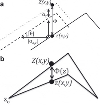
Regarding Figure 2a, the planimetric biases between the DEM and altimeter surfaces, represented by Z(x, y) and z(x, y), respectively, can be described by the offset vector ![]() and the surface slope θ. The offset vector consists of both horizontal (αxy
) and vertical (αz
) contributions, and assuming a constant surface slope over the distance |αxy
|, the total vertical offset between the DEM and altimeter surfaces is
and the surface slope θ. The offset vector consists of both horizontal (αxy
) and vertical (αz
) contributions, and assuming a constant surface slope over the distance |αxy
|, the total vertical offset between the DEM and altimeter surfaces is
where the model residual is given by ϵ.

Fig. 2. Planimetric and elevation-dependent corrections necessaryto apply when combining stereoscopic DEMs (Z(x, y)) with altimeter data (z(x, y)). (a) Planimetric offset. The total positional offset, Φ, is given as the sum of the contributions from the product of the horizontal offset, |αxy |, with the surface slope, θ, and the vertical offset, αz . (b) Principle behind the elevation-dependent offset.
By iteratively minimizing the offsets and discarding outliers greater than 2σ from the mean, the DEM is shifted in space until α reaches a minimum. The minimum value is chosen to be 1 m, and the result is a minimized root-meansquare error (RMSE) between the datasets. Following planimetric correction, we remove any elevation-dependent bias (Fig. 2b), which is assumed linear, through least-squares regression between the elevation and 4). The result is the DEM adjusted to the best fit, in a least-squares sense, with the altimeter data. By subtracting the altimeter elevations from the DEM observations in the points (x, y), the residuals are found to be normally distributed around a mean of 0 m (Fig. 3a and b).

Fig. 3. Input data and results from JI. (a) 2008 residuals given as DEM minus altimeter elevations in the altimeter observation points. The red areas show regions where the DEM elevations are higher, and the blue where they are lower. (b) The residuals’ distribution in a histogram. (c, d) OLE interpolation values (c) and errors (d). (e, f) Using the 2007 and 2008 interpolation values to correct the corresponding DEMs, the intermediate surface elevation changes (e) and error estimates (f) are found.
3.2. Spatial interpolation
Following least-squares adjustment, we expand on the approach of Reference Nuth and KääbNuth and Kääb (2011) in order to further improve the DEM through interpolation and extrapolation of the residual differences with the altimeter elevations. Residuals that exceed the DEM elevation errors of approximately ±12 m are treated as outliers and discarded, while geostatistical techniques are used to spatially interpolate the remaining residuals to cover the entire observation area. This allows one to gain a full overview of the offset introduced due to the different acquisition times of the SPOT image relative to the ATM and ICESat data. The interpolation gives both interpolated residuals, dz est, and error variances. Taking the square root of the latter yields the RMSE, dz sig. Linearly interpolating the adjusted DEM to the prediction points gives Z intp, and the final, corrected, elevations are then found as
By directly differencing the 2007 and 2008 elevations and converting the results to m a−1, the intermediate elevation changes, dH/dt, are found.
Multiple interpolation methods are tested in order to find the one providing the most realistic result, i.e. prediction values that reproduce the residuals as accurately as possible without also producing a too smooth surface between the observation points. The methods are simple and ordinary kriging as well as OLE in the form of least-squares collocation (Reference Hofmann-Wellenhof and MoritzHofmann-Wellenhof and Moritz, 2005). Kriging is performed using the MATLAB toolbox mGstat while OLE is performed with the Fortran-based GRAVSOFT program GEOGRID (Reference Forsberg and TscherningForsberg and Tscherning, 2008; Reference HansenHansen, 2011). A spherical semivariogram or a second-order Markov covariance model, respectively, is applied to the residuals found for each observation area for each year. All methods are linear, unbiased estimators, which minimize the estimation variance and return the input observation values for the observation points. In the case of a second-order stationary system, where the mean, variance and covariance are spatially constant, the methods are linked through the relation
where ![]() is the semi-variance,
is the semi-variance, ![]() the variance,
the variance, ![]() the covariance and
the covariance and ![]() is the distance between two observations, i.e. the lag distance. If two measurements are conducted in close proximity to each other, they are assumed to have similar values. For a small lag, they are thus highly correlated, in which case the covariance is high and the semi-variance low.
is the distance between two observations, i.e. the lag distance. If two measurements are conducted in close proximity to each other, they are assumed to have similar values. For a small lag, they are thus highly correlated, in which case the covariance is high and the semi-variance low.
For both methods, data errors are included by adding a semivariogram or variance–covariance matrix to the observations. We do not, however, create different semivariograms or variance–covariance matrices depending on the surface type as has been suggested by Reference Rolstad, Haug and DenbyRolstad and others (2009). They found different semivariogram parameters for steep and flat blue ice, snow and bedrock, respectively, as the surface type determines the spatial correlation between observations spaced by ![]() . Data clustering is accounted for through a weighting based on the data configuration and their respective covariances/semi-variances rather than the actual observation values. Note that SK and OLE are essentially two ways of performing the same calculations (Reference DermanisDermanis, 1984; Reference Hofmann-Wellenhof and MoritzHofmann-Wellenhof and Moritz, 2005; Reference NielsenNielsen, 2009).
. Data clustering is accounted for through a weighting based on the data configuration and their respective covariances/semi-variances rather than the actual observation values. Note that SK and OLE are essentially two ways of performing the same calculations (Reference DermanisDermanis, 1984; Reference Hofmann-Wellenhof and MoritzHofmann-Wellenhof and Moritz, 2005; Reference NielsenNielsen, 2009).
4. Results
Having spatially interpolated the residuals, similar results are found from the three techniques. A few differences are, however, evident, for example at JI where generally lower OLE errors ranging from ±0.3 to 5.2 m a−1 are obtained compared to the kriging errors, which range from ±3.6 to 7.6 m a−1. Furthermore, kriging yields unrealistically smooth interpolation surfaces, while SK and OLE produce different results in spite of being constructed from the same set of equations. These differences are explained by the covariance model being of better quality than the variogram model, since the former implements the covariances directly while the latter uses a spherical semivariogram model fitted to the empirical values and thus does not include the residuals’ oscillation above and below 0 m. The results presented in the following are therefore based on OLE.
An example of the residuals for the 2008 data at JI is shown in Figure 3a and b, while Figure 3c and d show the OLE interpolation values and RMSE, respectively. Table 1 summarizes the results in numbers. During the registration, the horizontal and vertical offsets are reduced from the decimeter level to the cm level, and during this process observations for which the residuals exceed the DEM errors of ∼12 m are treated as outliers and discarded. This reduces the number of data points (Fig. 3a relative to Fig. 1c) and results in residuals normally distributed around zero. The largest negative offsets are found along the flow channel where the largest surface changes occur. As the August DEM is registered to ATM data from June/July, the intermediate lowering of the surface will yield negative residuals when subtracting the altimeter observations from the DEM. Further inland, the offsets are closer to zero, while some positive values are also found. These can be explained by errors in the DEMs (Reference Korona, Berthier, Bernard, Rémy and ThouvenotKorona and others, 2009). The RMSE ranges from 0.2 to 4.6 m, with the lowest values coinciding with the position of the altimeter points, and the greater the distance to these, the larger the error. It is found that for flights ∼10 km apart, the errors range from 0.2 to 2 m, while when the distance between ground tracks halves, the error approximately halves accordingly. As will become clearer from the elevation change maps presented below, this relation is important when planning the spatial density of airborne flights in order to estimate surface changes in areas of varying topography, such as at outlet glaciers.
Table 1. Statistics on residuals (Φ) and interpolation results after applying optimal linear estimation to obtain dz est and dz sig

The surface elevations and elevation changes are found using Eqn (1), and as data errors are taken into account during the interpolation, Gaussian quadratic summation can be applied to the 2007 and 2008 RMSE values to give the dH/dt error estimates, σ dH/dt. The results are presented in Figures 3e and f andFig 4a and b as well as in Table 2. The data gaps in the figures result from errors as well as the application of cloud and rock masks during the initial manual editing of the DEMs. For JI (Fig. 3e), a large area with dH/dt ≈ −35 m a−1 marks the glacier basin. Surrounding this, the flow channel is distinguishable with dH/dt between −25 and −10 m a−1 and values increasing further inland. This large lowering agrees well with the mass loss reaching a maximum of 34 Gt a−1 by the end of 2007, after which it fluctuates between 25 and 33 Gt a−1 (Reference Howat, Ahn, Joughin, Van den Broeke, Lenaerts and SmithHowat and others, 2011). At higher elevations further east, the pattern of dH/dt changes with values of approximately or slightly above 0 m a−1, indicating a steady or slowly rising surface. The errors (Fig. 3f) range from ±0.3 to 5.2 m a−1, the lowest values being found nearest to the altimeter ground tracks, after which they increase with distance from there.

Fig. 4. Surface elevation changes (a) and error estimates (b) from KL from 2007 to 2008.
Table 2. Surface elevation change (m a−1) results from the two glaciers. The last column gives the elevation change error found by applying quadratic summation to the 2007 and 2008 interpolation errors
At KL (Fig. 4a), negative elevation changes are found throughout most of the observation area, making the flow pattern clearly noticeable. The glacier basin and the area north of it experienced a large lowering of dH/dt between −25 and −10 m a−1 . Higher elevations to the east and southwest are less affected by recent changes in ice flow, so dH/dt ≈ 0 m a−1. The positive values scattered around the flow channel and drainage basin are believed to result from melt lakes on the ice as well as a major retreat ending in 2005–06, after which the front stabilized (Reference Howat, Ahn, Joughin, Van den Broeke, Lenaerts and SmithHowat and others, 2011). The errors span ±0.3–5.1 m a−1 (Fig. 4b). The minimum is found in the vicinity of approximately overlapping altimeter ground tracks, i.e. in the glacier basin with the minimum values depicting the overlap. Unfortunately, there are no observations in the area immediately north/ northwest of the basin where dH/dt < 0 m a−1. This is reflected in generally higher errors, i.e. σ dh / d t = ±12.9–5.1 m a−1. It also explains the greater number of higher errors at KL than at JI where altimeter data cover a larger part of the observation area.
5. Discussion
Both kriging and OLE are linear, unbiased estimators that take data clustering into account when spatially interpolating a set of measurements. Thus, the interpolation depends on the spatial distribution of data rather than their actual values, and the formation of a spatially varying mean of the observation values is allowed. The results indicate a clear relationship between the distribution of altimeter data and the errors: the denser the grid of observations, the more accurate the predictions based on the neighbourhood, and the lower the errors. Figure 5 illustrates this relationship for the OLE interpolation errors, and as these are used to produce the dH/dt errors, this distance dependence translates directly. This observation is crucial in planning future airborne surveys as it can be used to ensure that flights are carried out in grids dense enough to ensure minimum errors. The reason for the low errors relative to the data errors is the referencing of the DEMs to altimeter observations agreeing in time and space, as well as OLE being based on a well-defined covariance model which takes data errors into account. The spatial structure of the DEM errors is not accounted for, however, as we only had point-wise errors in the estimation points. This may explain the positive residuals found at JI when registering the August 2008 DEM to June/July ATM data. Another possible explanation is that we have not accounted for different surface types, such as steep/flat blue ice and snow, giving different semivariograms/variance–covariance matrices (Reference Rolstad, Haug and DenbyRolstad and others, 2009). This changes the parameters in the models used for the interpolation if, for example, steep slopes indicate less spatial correlation between the observation points. In spite of this, our results agree well with those obtained by Reference Howat, Ahn, Joughin, Van den Broeke, Lenaerts and SmithHowat and others (2011), who estimated surface mass-balance changes for the period 2000–10 for Helheim, KL and JI using the Regional Atmospheric Climate MOdel version 2 (RACMO2) as described by Reference EttemaEttema and others (2009, Reference Ettema, Van den Broeke, Van Meijgaard, Van de Berg, Box and Steffen2010). Reference Howat, Ahn, Joughin, Van den Broeke, Lenaerts and SmithHowat and others (2011) found that a major front retreat ended in 2005–06, after which the front stabilized. This supports the patchy thickening of KL’s glacier basin. When considering elevation changes derived from ATM only (Fig. 6), we observe a trend similar to ours: a lowering of JI’s trunk of ∼25 m a−1, ∼10 m a−1 further up the channel, and values of ∼0 m a−1 and below at higher elevations north of the flow channel. We thus have confidence in our results.

Fig. 5. Estimate of accuracy of OLE as a function of the distance to the closest altimeter point. As the accuracy estimates are used to find the surface elevation change errors, this relationship translates directly. (a) JI and (b) KL.

Fig. 6. ATM elevation changes between May 2007 and June/July 2008 for validation purposes: (a) JI and (b) KL.
As the laser data and DEMs are not acquired at exactly the same time of the year, an error is introduced due to the seasonal signal of the ice. However, as the DEMs are co-registered to altimeter ICESat and ATM data, several limitations emerge, which complicate or prevent the acquisition of all the data simultaneously: ICESat’s orbit limited the spatial and temporal distribution of flights, and ATM is flown according to logistics, weather and target priorities. Furthermore, the SPIRIT campaign was of short duration and only focused on certain parts of the Greenland ice sheet. As the JI DEMs are co-registered to altimeter data acquired from April to October and the DEMs from KL are separated by 14 months, it is not valid to assume that the seasonal elevation cycle was eliminated from the difference data. One path to mitigating the effects arising from surface processes is through the use of a coupled surface energy and meteorological reanalysis model such as that by Reference Van den Broeke, Bus, Ettema and SmeetsVan den Broeke and others (2010). By applying such an approach, even sharper Gaussian curves will be found than those from this analysis, (Fig. 3b). In spite of this, part of the information contained in the residuals is exactly the offset resulting from different temporal resolutions. Spatially interpolating the offsets over the entire observation area demonstrates the strength of our model: it provides the ability to identify and correct offsets using geostatistical interpolation, thereby improving the DEM elevations and DEM differences.
The combination of datasets described here may be generally applicable to many other data sources (e.g. Envisat, CryoSat-2 and the Advanced Spaceborne Thermal Emission and Reflection Radiometer (ASTER)). Once airborne and validated, data from ICESat-II can also be employed. CryoSat-2 data are becoming available to the scientific community at the time of writing, while Envisat operated from 2002 until April 2012, yielding a vast number of data from its 35 day repeat track period. Although it is necessary to account for backscattering effects and the radar signal’s penetration into the firn, work is ongoing in order to fully understand the implications, such as through CryoVex, the CryoSat-2 validation campaign carried out using both laser and radar altimetry (Reference Drinkwater and RebhanDrinkwater and Rebhan, 2003). NASA’s Land, Vegetation, and Ice Sensor (LVIS) has been flown over most of Greenland’s west and southeast coasts as part of Operation IceBridge, and GPS receivers are deployed on the ice by outlet glaciers such as JI and Russell Glacier. As they provide continuous and very accurate position and elevation estimates, the inclusion of such data will be beneficial for ensuring consistently high-accuracy estimates (Reference Joughin, Das, King, Smith, Howat and MoonJoughin and others, 2008; Reference Shepherd, Hubbard, Nienow, McMillan and JoughinShepherd and others, 2009; Reference Khan, Wahr, Bevis, Velicogna and KendrickKhan and others, 2010). Satellite imagery is available from, for example, the ASTER sensor on board the Terra satellite. Such data have been available since 1999, and numerous projects aimed at estimating surface changes in ice-covered regions have been conducted (Reference Howat, Joughin and ScambosHowat and others, 2007; Reference KääbKääb, 2008). Thus, although the SPIRIT campaign has finished and ICESat is no longer operating, there is a possibility of continuously constraining DEMs using more accurate data-sets to increase the spatial resolution and decrease the errors of surface elevation maps, particularly in areas of a rough surface topography.
6. Conclusions
This work focused on developing a method for estimating elevation changes with a high spatial resolution in areas with rapid surface changes such as outlet glaciers. This involved a combination of stereoscopic DEMs from SPOT 5 and laser altimeter data from ICESat and ATM, and the test regions were the two Greenlandic outlet glaciers Jakobshavn Isbræ and Kangerdlugssuaq over the period 2007–08. The goal was to co-register the DEMs to altimeter data as they agreed in time and space. The altimeter elevation error was one order of magnitude smaller than that of the DEM, 10–15 cm, thus representing a good approximation of the true surface. By moving the DEM in space until it agreed with the laser data and applying geostatistical interpolation in the form of optimal linear estimation, it became possible to correct the DEMs for the offsets relative to the altimeter surfaces. In this way, elevation maps were produced with a spatial resolution of 100 m and elevation errors no higher than 14.6 m (JI 2007). Simple and ordinary kriging were also applied, but led to significantly poorer results. The method allowed detailed information to be obtained regarding the surface topography throughout the observation areas, i.e. not only along but also between the altimeter flight lines and ground tracks. It also reduced the estimation errors noticeably, particularly in the vicinity of altimeter observations. For flights ∼10 km apart, the errors ranged from ±0.2 to 2 m, and when halving the distance between ground tracks, the error halved accordingly.
By differencing two elevation maps, the temporal surface elevation changes were mapped, and for the given observation period a lowering of the terminus region and flow channel was observed for both glaciers. For JI, the terminus lowered by −35 to −30 m. The flow channel lowered by −25 to −10 m a−1, while the surrounding higher-elevation areas were approximately unchanged. For KL, part of the terminus lowered at rates of 20–25 m a−1 while the flow channel experienced a lowering of approximately −18 to −5 m a−1. The remaining surface rose by a few m a−1. The elevation change errors ranged from ±0.3 to 5.2 m a−1 for JI and ±0.3 to 5.1 m a−1 for KL, and as was the case in the interpolation the smallest errors were found in the vicinity of altimeter observations. A significant result was this strong dependence of the size of the errors on the position of the altimeter data: As the density of altimeter observations increased, the errors decreased significantly. Thus, as satellite orbits cannot be changed, for example, to observe short-term surface changes in specific areas, and because exact repeat tracks are rare, this relationship between flight lines and estimation errors is of great importance for airborne flight planning. Previous ATM ground tracks are often re-flown with a >50% overlap (Reference KrabillKrabill and others, 2002). When combined with knowledge of the error distribution, the combination of stereoscopic imagery and laser altimeter data, particularly acquired during airborne campaigns, enables continuous mapping of both accurate surface elevations and elevation changes in areas of rapidly changing ice surfaces.
Acknowledgements
The ICESat and ATM data were downloaded from the NSIDC website, and the SPOT 5-HRS imagery was obtained as part of the SPIRIT campaign launched by CNES, SPOT Image and LEGOS. J.F. Levinsen acknowledges I.M. Howat for receiving her into his research group at the School of Earth Sciences at The Ohio State University. The stay was made possible through a Fulbright scholarship. We thank the reviewers for constructive comments, which led to a significant improvement of the manuscript.