


1. Introduction
The ocean is a complex physical system due to the interaction of motions of different length and time scales. Nevertheless, long-lived coherent structures in the ocean are discernible in observational data. In particular, mesoscale vortices with typical horizontal scales of the order of 100 km may persist during several weeks or even months. The lifetime of such structures is affected by external forcing mechanisms, interactions with other oceanic features, and their intrinsic stability properties. An example is reported by Dewar (Reference Dewar2002), who discusses the evolution of meddies (i.e. sub-surface vortices of Mediterranean origin), which are affected by the shape of the seafloor. Careful observations of meddies suggest that interactions with topographic features may be disruptive and lead to vortex disintegration (Shapiro, Meschanov & Emelianov Reference Shapiro, Meschanov and Emelianov1995; Richardson & Tychensky Reference Richardson and Tychensky1998). A similar process is observed during the transit of Agulhas eddies over submarine ridges in the south-eastern Atlantic Ocean (Kamenkovich et al. Reference Kamenkovich, Leonov, Nechaev, Byrne and Gordon1996; Schouten et al. Reference Schouten, de Ruijter, van Leeuwen and Lutjeharms2000). The obstruction and eventual destruction of vortices encountering topographic obstacles in a rotating system have been studied in laboratory experiments (Zavala Sansón Reference Zavala Sansón2002; Zavala Sansón, Barbosa Aguiar & van Heijst Reference Zavala Sansón, Barbosa Aguiar and van Heijst2012) and numerical simulations (e.g. van Geffen & Davies Reference van Geffen and Davies2000; Zavala Sansón & Gonzalez Reference Zavala Sansón and Gonzalez2021).
Analytical models of coherent vortices are helpful to understand their general dynamics and stability properties, which can then be compared with realistic conditions. Here, we are interested in nonlinear vortical solutions in a rotating system, which are often used to model persistent structures in the oceans and atmosphere (van Heijst & Clercx Reference van Heijst and Clercx2009). Nonlinearities are a key ingredient that prevents vortex erosion in the form of planetary or topographic Rossby waves, which are generated in the presence of spatial variations of the planetary vorticity ( $\beta$ effect) or bottom topography, respectively. In the quasi-geostrophic (QG) context, a type of dipolar structures is the so-called ‘modon’ (Stern Reference Stern1975). Solutions of frontal oceanic eddies in a reduced-gravity model, known as ‘rodons’, were derived by Cushman-Roisin, Heil & Nof (Reference Cushman-Roisin, Heil and Nof1985). Azimuthal-mode solutions of multipolar, barotropic and baroclinic QG vortices were derived by Viúdez (Reference Viúdez2019a,Reference Viúdezb). Recently, Gonzalez & Zavala Sansón (Reference Gonzalez and Zavala Sansón2021) obtained nonlinear solutions of monopoles and dipoles over an isolated topographic feature. The latter will be considered in this work to study the stability of monopolar vortices trapped over seamounts and valleys.
The stability of monopolar vortices in a rotating system with no topography has been studied from different points of view. Gent & McWilliams (Reference Gent and McWilliams1986) investigated the linear instability of QG circular vortices with zero circulation in the  $f$-plane to azimuthal normal mode perturbations. The authors found that the fastest growing perturbations may be internal (with vertical structure) or external (barotropic) depending on the steepness of the stream function radial profile. A linearised contour dynamics model, used by Flierl (Reference Flierl1988), extended the analysis to baroclinic circular vortices. Rotating tank experiments and three-dimensional numerical simulations have shown that cyclonic and anticyclonic vortices may be subject to both barotropic (two-dimensional) and centrifugal (three-dimensional) instabilities (Kloosterziel & van Heijst Reference Kloosterziel and van Heijst1991; Orlandi & Carnevale Reference Orlandi and Carnevale1999). A necessary criterion for barotropic linear instability is obtained from Rayleigh's inflexion point theorem adapted to swirling flows (Gent & McWilliams Reference Gent and McWilliams1986). The authors found that isolated vortices (circular flows with zero net circulation) may be barotropically unstable and, for sufficiently steep vorticity profiles, develop a wavenumber two azimuthal perturbation transforming into tripolar structures. In rotating tank experiments, unstable cyclonic vortices typically form tripoles (van Heijst & Kloosterziel Reference van Heijst and Kloosterziel1989). Higher wavenumbers leading to multipolar vortices are also possible (Carnevale & Kloosterziel Reference Carnevale and Kloosterziel1994; Trieling, van Heijst & Kizner Reference Trieling, van Heijst and Kizner2010; Cruz Gómez, Zavala Sansón & Pinilla Reference Cruz Gómez, Zavala Sansón and Pinilla2013). Anticyclones, in contrast, are prone to centrifugal instabilities and usually break into dipole pairs (Kloosterziel & van Heijst Reference Kloosterziel and van Heijst1991). The combined effects of barotropic and centrifugal instabilities were discussed thoroughly by Orlandi & Carnevale (Reference Orlandi and Carnevale1999). On the other hand, non-isolated vortices (with monotonic vorticity profiles) are barotropically stable (Kloosterziel & van Heijst Reference Kloosterziel and van Heijst1992).
Topographic features at the solid bottom can affect vortices with finite depth. Numerical and experimental studies have revealed different physical processes involved in the vortex–topography interactions. These include the radiation of topographic waves and the paths that monopolar and dipolar vortices follow around local topographies, such as seamounts and valleys (Carnevale, Kloosterziel & van Heijst Reference Carnevale, Kloosterziel and van Heijst1991). Oceanic eddies are often eroded or divided when encountering a tall seamount (Herbette, Morel & Arhan Reference Herbette, Morel and Arhan2002, Reference Herbette, Morel and Arhan2005; Sutyrin, Herbette & Carton Reference Sutyrin, Herbette and Carton2011) or a submarine ridge (van Geffen & Davies Reference van Geffen and Davies1999; Zavala Sansón Reference Zavala Sansón2002). In some cases, vortical structures can be trapped over the topography (Zavala Sansón et al. Reference Zavala Sansón, Barbosa Aguiar and van Heijst2012; Zavala Sansón & Gonzalez Reference Zavala Sansón and Gonzalez2021), and a natural question concerns the stability of such configurations. Carton & Legras (Reference Carton and Legras1994) studied the stability of shielded circular vortices over an axisymmetric parabolic bottom, and found that if the vortex core is cyclonic, then a compact and stable tripolar structure emerges. In contrast, the tripoles formed from anticyclonic vortices are unstable and break into two dipoles moving in opposite directions. Nycander & Lacasce (Reference Nycander and Lacasce2004) used generalised variational principles to find stable regimes for monopolar barotropic vortices over topography when the potential vorticity profiles are monotonic. In that case, the authors found a large set of stable anticyclonic and cyclonic vortices over a circular seamount. Zhao, Chieusse-Gérard & Flierl (Reference Zhao, Chieusse-Gérard and Flierl2019) studied the stability of a barotropic Rankine vortex over a cylindrical topography and found that anticyclones are destabilised by seamounts and stabilised by depressions. These results were based on the assumption that the potential vorticity is a piecewise constant function. The jumps in the potential vorticity arose from both the cylindrical topography and the relative vorticity profile. The linear stability of another piecewise circular flow around a rigid cylindrical ‘island’ with conical topography was studied by Rabinovich, Kizner & Flierl (Reference Rabinovich, Kizner and Flierl2018), and the resulting nonlinear evolution by Rabinovich, Kizner & Flierl (Reference Rabinovich, Kizner and Flierl2019). In these studies, the authors discuss the stabilising/destabilising role of the bottom slope on clockwise and anticlockwise flows.
This work studies the linear stability of barotropic monopolar vortices over isolated topography. In the first part (§ 2), we pose the problem of a circular flow perturbed by azimuthal normal modes, and derive a generalised eigenvalue problem for the corresponding growth rates. The analysis is carried out for flows under the shallow-water (SW) approximation and extended to the QG dynamics. Then extensions of classical theorems for barotropic and centrifugal instabilities taking topographic effects into account are presented. In the second part (§ 3), we study numerically the stability of circular vortices over axisymmetric topography in the QG limit. The background flow is based on the recent QG solutions obtained by Gonzalez & Zavala Sansón (Reference Gonzalez and Zavala Sansón2021), which represent both cyclones and anticyclones over mountains and valleys, and whose potential vorticity is not uniform. A relevant feature of the solutions is that the bottom topography is arbitrary, subject only to the restriction of being axisymmetric and isolated (the bottom topography becomes flat at large radii). The theoretical results are contrasted with the spectral solution of the corresponding generalised eigenvalue problem. In addition, we perform QG numerical simulations initialised with different vortex–topography configurations. Finally, conclusions are discussed in § 4.
2. Stability of monopolar vortices over axisymmetric topography
2.1. Linear analysis for SW and QG flows
This subsection examines the linear stability problem associated with the SW model on the  $f$-plane, including topographic effects and under the rigid-lid approximation. Using polar coordinates $(r,\theta )$ and assuming an axisymmetric topography, a single fluid layer in this system satisfies the vorticity equation
 \begin{equation} h_{s}\,\frac{\partial q_s}{\partial t} + J(\psi_s,q_s) = 0, \end{equation}
where  $\psi _s$ represents the transport function, and $q_s=h_s^{-1}(\omega _s + f_0)$ is the potential vorticity (PV), with $\omega _s = \boldsymbol {\nabla } \boldsymbol {\cdot } (h_s^{-1}\,\boldsymbol {\nabla } \psi _s)$ the relative vorticity, and $f_0$ the Coriolis parameter. Also, $J(a,b)=(\partial _r a\,\partial _{\theta }b -\partial _{\theta }a\, \partial _r b )/r$ is the Jacobian operator, and $h_s(r) = H_0 - b(r)$ is the fluid layer thickness, where $b(r)$ is the axisymmetric topographic profile with amplitude $b_0$ and horizontal scale $r_t$, and $H_0$ is the average depth of the fluid layer (figure 1). We consider isolated topographies, ${\rm d}b/{\rm d}r\rightarrow 0$ for $r\gg r_t$, which can be mountains ( $b_0>0$) or valleys ( $b_0<0$). Under the rigid-lid approximation, the temporal variations of the layer thickness are ignored in the continuity equation, so surface gravity waves are suppressed. The radial and azimuthal velocity components are defined as $u_s = -(h_s r)^{-1}\,\partial _{\theta }\psi _s$ and $v_s = h_s^{-1}\,\partial _r \psi _s$.

Figure 1. Side view of a fluid layer with mean depth  $H_0$ over bottom topography $b(r)$ defined as an axisymmetric submarine mountain or valley of amplitude $b_0$ and width $r_t$ on an $f$-plane.
A linear stability analysis is used to introduce small, two-dimensional disturbances  $\psi _s'(r,\theta,t)$ on a basic flow $\varPsi _s(r)$, which represents a steady, axisymmetric solution of (2.1):
 \begin{equation} \psi_s(r,\theta,t) = \varPsi_s(r) +\psi_s'(r,\theta,t).\end{equation}
The basic flow can be a circular cyclonic or anticyclonic vortex swirling above the topography, which can be a mountain or a valley. Note that the potential vorticity can be written as
 \begin{equation} q_s(r,\theta,t) = Q_s(r) +q_s'(r,\theta,t),\end{equation}
where  $Q_s=h_s^{-1}[\boldsymbol {\nabla } \boldsymbol {\cdot } (h_s^{-1}\,\boldsymbol {\nabla } \varPsi _s) +f_0]$ is the basic PV, and $q_s'=h_s^{-1}\,\boldsymbol {\nabla } \boldsymbol {\cdot } (h_s^{-1}\,\boldsymbol {\nabla } \psi _s')$ is its perturbation. Inserting (2.2) and (2.3) into the vorticity equation (2.1) and linearising:
 \begin{equation} h_s\,\frac{\partial q_s'}{\partial t} + J(\varPsi_s,q_s') + J(\psi_s',Q_s) = 0. \end{equation}
The disturbance is assumed of the form
 \begin{equation} \left. \begin{array}{c@{}} \psi_s'(r,\theta,t) = \phi(r)\,{\rm e}^{{\rm i}(k\theta - \sigma t)}, \\ q_s'(r,\theta,t) = \dfrac{1}{h_s}\,\mathcal{L}_{s}[\phi(r)] \,{\rm e}^{{\rm i}(k\theta - \sigma t)}, \end{array}\right\} \end{equation}
where  $\mathcal {L}_s[\ ]$ is a differential operator defined by $\mathcal {L}_s = r^{-1}\,\partial _r(rh_s^{-1}\,\partial _r) - r^{-2}h_s^{-1}k^2$, $k$ is the azimuthal wavenumber, $\phi (r)$ is a complex amplitude, and $\sigma =\sigma _r + \textrm {i}\sigma _i$ is a complex number whose real part is the frequency of the disturbance, and the imaginary part represents its growth rate. The condition for instability is that the growth rate $\sigma _i$ is positive.
Applying (2.5) to (2.4) provides the generalised eigenvalue problem
 \begin{equation} \sigma \mathcal{L}_{s}\phi = \frac{k}{r}\left[\frac{\partial_r \varPsi_s}{h_s}\,\mathcal{L}_{s} - \partial_r Q_s \right]\phi. \end{equation}
The matrix representation of this equation is given by
 \begin{equation} \sigma \boldsymbol{\mathsf{A}}\,\phi(r) = \boldsymbol{\mathsf{B}}\,\phi(r),\end{equation}
where  $\boldsymbol{\mathsf{A}}$ and $\boldsymbol{\mathsf{B}}$ are non-Hermitian and real matrices, $\sigma$ is the eigenvalue, and $\phi$ is the eigenfunction. Solutions of (2.6) for different wavenumbers $k$ provide the eigenvalues and, consequently, the growth rate of the corresponding perturbation. However, analytical solutions are often difficult to obtain, so the problem is usually solved numerically, as we will do in § 3.
Now we examine the QG dynamics obtained when the layer thickness is much greater than the amplitude of the topography,  $H_0 \gg b_0$ (Vallis Reference Vallis2017). In this case, the vorticity equation is
 \begin{equation} \frac{\partial}{\partial t}\nabla^2 \psi + J(\psi,q) = 0,\end{equation}
where now  $\psi =\psi _s/H_0$ is the stream function, and $q=\omega +h(r)$ is the QG PV, with $\omega =\nabla ^2\psi$ the relative vorticity, and $h(r)=f_0H_0^{-1}\,b(r)$ the ambient vorticity (Zavala Sansón & van Heijst Reference Zavala Sansón and van Heijst2014). The radial and azimuthal velocity components are now defined as $u = -r^{-1}\,\partial _{\theta }\psi$ and $v =\partial _r \psi$, respectively.
The perturbed flow is of the form
 \begin{equation} \psi(r,\theta,t) = \varPsi(r) +\psi'(r,\theta,t), \end{equation}
where  $\varPsi$ ( $=\varPsi _s/H_0$) is the basic flow, and $\psi '$ is a small perturbation. Applying the same linear analysis used for the SW equations, we obtain the generalised eigenvalue problem
 \begin{equation} \sigma \mathcal{L} \phi = \frac{k}{r}\,[\partial_r \varPsi \mathcal{L} - \partial_r (\nabla^2\varPsi + h)]\phi, \end{equation}
where the linear operator is  $\mathcal {L}=\partial _{rr} + r^{-1}\,\partial _r - r^{-2}k^2$. This expression for QG can be compared with the SW version (2.6).
2.2. Barotropic instability
Barotropic instability refers to growing disturbances that arise on shear flows. A necessary criterion for instability is provided by Rayleigh's inflexion point theorem for either parallel or circular two-dimensional flows (Gent & McWilliams Reference Gent and McWilliams1986). A more restrictive (yet necessary) criterion is given by Fjørtoft's theorem. This subsection presents a new version of these theorems for circular vortices over topography.
2.2.1. Rayleigh's inflexion point theorem with topography
The generalised eigenvalue problem (2.6) in the SW model can provide an equivalent of Rayleigh's inflexion point theorem involving topography effects. First, (2.6) is rewritten as
 \begin{equation} \frac{{\rm d}}{{\rm d}r}\left(\frac{r}{h_s}\,\frac{{\rm d} \phi}{{\rm d}r} \right) - \frac{k^2}{rh_s}\,\phi - \frac{d_rQ_s}{r^{{-}1}h_s^{{-}1}\,d_r\varPsi_s - \sigma/k}\,\phi = 0, \end{equation}
where  $d_r \equiv {\textrm {d}}/{\textrm {d}r}$. Note that (2.11) assumes $r^{-1}h_s^{-1}\,d_r\varPsi _s - \sigma /k \neq 0$ to avoid trivial solutions of $\phi$ (because $d_rQ_s\neq 0$ in general). Multiplying this equation by the complex conjugate $\phi ^*$, integrating each term, and applying the null boundary conditions at $r = 0$ and $r = r_{m} \rightarrow \infty$ (the maximum value in the radial direction), both obtained from the asymptotic analysis for small and large $r$ (Gent & McWilliams Reference Gent and McWilliams1986), yields
 \begin{equation} \int_0^{r_m}\frac{r}{h_s}\,|d_r\phi|^2\, {\rm d} r + \int_0^{r_m}\frac{k^2}{rh_s}\,|\phi|^2\, {\rm d} r + \int_0^{r_m}\frac{(r^{{-}1}h_s^{{-}1}\,d_r\varPsi_s - \sigma^*/k)\,d_rQ_s}{|r^{{-}1}h_s^{{-}1}\,d_r\varPsi_s - \sigma/k|^2}\,|\phi|^2\, {\rm d} r=0.\end{equation}
The imaginary part of (2.12) is
 \begin{equation} \frac{\sigma_i}{k}\int_0^{r_{m}} \frac{ d_rQ_s}{|r^{{-}1}h_s^{{-}1}\,d_r\varPsi_s - \sigma/k|^2}\,|\phi|^2 \, {\rm d} r = 0. \end{equation}
If  $\sigma _i \neq 0$, then the basic flow could be unstable. In this case, to satisfy (2.13), the potential vorticity gradient must be zero at some $r=r_z$, i.e.
 \begin{equation} \left.\frac{{\rm d}}{{\rm d}r} \left[\frac{\boldsymbol{\nabla} \boldsymbol{\cdot} (h_s^{{-}1}\,\boldsymbol{\nabla} \varPsi_s) + f_0 }{h_s} \right] \right|_{r=r_z} =0, \end{equation}
which is a necessary criterion of instability for the SW model. In the QG limit, the result is equivalent but now using the QG PV:
 \begin{equation} \left.\frac{{\rm d}}{{\rm d}r} [\nabla^2 \varPsi + h(r) ] \right|_{r=r_z} =0. \end{equation}
Note that for the flat-bottom case,  $h(r) = 0$, condition (2.15) demands the relative vorticity gradient to be null at some radial distance, as reported by Gent & McWilliams (Reference Gent and McWilliams1986).
2.2.2. Fjørtoft's theorem with topography
Here, we present an equivalent criterion of Fjørtoft's theorem with topography in the SW model. First, note that the real part of (2.12) allows us to find
 \begin{equation} \int_0^{r_m}\frac{d_rQ_s\,(r^{{-}1}h_s^{{-}1}\,d_r\varPsi_s -\sigma_r/k)}{|r^{{-}1}h_s^{{-}1}\,d_r\varPsi_s - \sigma/k|^2}\,|\phi|^2 \, {\rm d} r < 0. \end{equation}
Second, if  $\sigma _i \neq 0$ and condition (2.13) is satisfied, then
 \begin{equation} (r^{{-}1}h_s^{{-}1}\,d_r\varPsi_s|_{r=r_z} - \sigma_r/k)\int_0^{r_m}\frac{d_rQ_s}{|r^{{-}1}h_s^{{-}1}d_r\,\varPsi_s - \sigma/k|^2}\,|\phi|^2 \, {\rm d} r = 0. \end{equation}
Subtracting (2.17) from (2.16), we obtain
 \begin{equation} \int_0^{r_m}\frac{d_rQ_s\,(r^{{-}1}h_s^{{-}1}\,d_r\varPsi_s - r^{{-}1}h_s^{{-}1}\,d_r\varPsi_s|_{r=r_z})}{|r^{{-}1}h_s^{{-}1}\,d_r\varPsi_s - \sigma/k|^2}\,|\phi|^2 \, {\rm d} r < 0, \end{equation}
which, to be satisfied, requires that the numerator of the integrand be negative for some  $r$:
$r$:
 \begin{equation} \frac{{\rm d}}{{\rm d}r}\left[\frac{\boldsymbol{\nabla} \boldsymbol{\cdot} (h_s^{{-}1}\,\boldsymbol{\nabla} \varPsi_s) + f_0}{h_s}\right]\left(\frac{1}{rh_s}\,\frac{{\rm d} \varPsi_s}{{\rm d}r} - \frac{1}{r_z\,h_s(r_z)}\left.\frac{{\rm d} \varPsi_s}{{\rm d}r}\right|_{r=r_z}\right) < 0. \end{equation}
This expression indicates that circular flow over topography could be unstable if the sign of the velocity relative to the inflexion point is opposite to the sign of the potential vorticity derivative somewhere.
In the QG approximation, the instability criterion (2.19) is rewritten as
 \begin{equation} \frac{{\rm d}}{{\rm d}r}[\nabla^2\varPsi + h(r)]\left(\frac{1}{r}\,\frac{{\rm d} \varPsi}{{\rm d}r} - \frac{1}{r_z}\left.\frac{{\rm d} \varPsi}{{\rm d}r}\right|_{r=r_z}\right) < 0.\end{equation}
When there is no topography,  $h(r) = 0$, (2.20) is reduced to the theorem reported by Gent & McWilliams (Reference Gent and McWilliams1986) for circular flow. Notice that Fjørtoft's theorem (2.20) requires that the point $r = r_z$, where Rayleigh's theorem is satisfied, exists.
2.3. Centrifugal instability
Vertical motions in a three-dimensional swirling flow are able to trigger centrifugal instabilities (Orlandi & Carnevale Reference Orlandi and Carnevale1999). Rayleigh's circulation theorem provides a criterion to identify this type of instability (Kloosterziel & van Heijst Reference Kloosterziel and van Heijst1991). The criterion is based on energetic considerations for an axisymmetric flow with an arbitrary azimuthal velocity  $v(r)$ in the absence of viscosity, stratification and rotation, and with a flat bottom. An extension of the theorem including rotation effects was presented in Kloosterziel (Reference Kloosterziel1990) and Kloosterziel & van Heijst (Reference Kloosterziel and van Heijst1991), based on the conservation of angular momentum of fluid elements subjected to infinitesimal displacements. By following a similar analytical procedure, in this subsection we present an extension of the circulation theorem including topography effects. Note that centrifugal instability is inherently three-dimensional, in contrast with the purely two-dimensional barotropic instability examined above.
Consider the momentum equations of a circularly symmetric flow in cylindrical coordinates  $(r,\theta,z)$ on the $f$-plane:
 \begin{gather} \frac{{\rm D}u}{{\rm D}t} - f_0v - \frac{v^2}{r} ={-}\frac{1}{\rho}\,\frac{\partial P}{\partial r}, \end{gather}
 \begin{gather}\frac{{\rm D}v}{{\rm D}t} + f_0 u + \frac{uv}{r} = 0, \end{gather}
 \begin{gather}0 ={-}\frac{1}{\rho}\,\frac{\partial P}{\partial z} - g, \end{gather}
where  $(u,v)$ are the radial and azimuthal velocity components, $P(r,z)$ is the pressure, $g$ is gravity, and $D/Dt = \partial /\partial t + u\,\partial /\partial r + w\,\partial /\partial z$ is the material derivative, with $w$ the vertical velocity. The pressure is $\theta$-independent because the flow maintains its circular shape. The flow is assumed to maintain the hydrostatic balance in the vertical direction (as in the SW approximation).
Now consider the presence of the axisymmetric topography  $b(r)$ shown in figure 1. Integrating (2.23) from an arbitrary level $z$ and the surface, the pressure is
 \begin{equation} P=\rho g[h_s(r) + b(r)] - \rho g z. \end{equation}
The first term,  $p(r)=\rho g\,h_s(r)$, is the pressure associated with the surface elevation (which is neglected only in the continuity equation under the rigid-lid approximation). The horizontal momentum equations are rewritten as
 \begin{gather} \frac{{\rm D}u}{{\rm D}t} = \frac{v^2}{r} + f_0v -\frac{1}{\rho}\,\frac{{\rm d} p}{{\rm d}r} - g\,\frac{{\rm d} b}{{\rm d}r} , \end{gather}
 \begin{gather}\frac{{\rm D}}{{\rm D}t}\left(vr + \frac{1}{2}\,f_0r^2\right) = 0, \end{gather}
where (2.26) represents the conservation of absolute angular momentum.
As a basic flow, we assume a circular monopolar vortex with azimuthal velocity  $v(r)$. Following Kloosterziel & van Heijst (Reference Kloosterziel and van Heijst1991), we consider a fluid element that is displaced from $r = r_0$ to $r' = r_0 + \delta r$ without changing the pressure field $p(r)$ (in this sense the displacement is considered as virtual). The new azimuthal velocity is $v'(r')$. Using the conservation law (2.26) yields
 \begin{equation} v'(r')\,r' + \tfrac{1}{2}\,f_0r'^2 = v(r_0)\,r_0 + \tfrac{1}{2}\,f_0r_0^2.\end{equation}
The radial acceleration due to the virtual displacement is obtained from (2.25) as the variation of the acceleration between both states (disturbed and basic) evaluated at  $r'$:
$r'$:
 \begin{equation} \frac{{\rm D}^2\delta r}{{\rm D}t^2} = \left. \left( \frac{{\rm D}u'}{{\rm D}t} - \frac{{\rm D}u}{{\rm D}t}\right)\right|_{r=r'}. \end{equation}
Using (2.25), and after some manipulations,
 \begin{align} \frac{{\rm D}^2 \delta r}{{\rm D}t^2} &= \left[\frac{v'(r')^2}{r'} + f_0\,v'(r') -\frac{v(r')^2}{r'} - f_0\,v(r')\right] -g\delta\,\frac{{\rm d} b}{{\rm d}r} \nonumber\\ &= \frac{1}{r'^3} \left[ \left(v'(r')\,r' + \frac12\,f_0r'^2\right)^2 - \left(v(r')\,r' + \frac12\,f_0r'^2\right)^2 \right] - g\delta\,\frac{{\rm d} b}{{\rm d}r}. \end{align}
Here,  $\delta \,\textrm {d}b/\textrm {d}r=\textrm {d}b/\textrm {d}r|_{r'} - \textrm {d}b/\textrm {d}r|_{r_0}$ is the variation of the topography gradient as the particle is displaced. Substituting the first term with (2.27) gives
 \begin{equation} \frac{{\rm D}^2 \delta r}{{\rm D}t^2} = \frac{1}{r'^3}\left[\left(v(r_0)\,r_0 + \frac{1}{2}\,f_0r_0^2\right)^2 - \left(v(r')\,r' + \frac{1}{2}\,f_0r'^2\right)^2 \right] - g\delta\,\frac{{\rm d} b}{{\rm d}r}. \end{equation}
A Taylor expansion close to  $r_0$ simplifies this expression to order $\delta r$:
 \begin{equation} \frac{{\rm D}^2 \delta r}{{\rm D}t^2} \sim{-}\delta r\,\frac{{\rm d}}{{\rm d}r}\left[ \frac{1}{r_0^3}\left(v(r)\,r + \frac{1}{2}\,f_0r^2\right)^2 + g\,\frac{{\rm d} }{{\rm d}r} b(r) \right]_{r=r_0}. \end{equation}
 If the fluid element is displaced outwards ( $\delta r>0$), then the acceleration (2.31) in that direction is positive when
 \begin{equation} \frac{{\rm d}}{{\rm d}r}\left[\frac{1}{r_0^3}\left(v(r)\,r + \frac{1}{2}\,f_0r^2\right)^2 + g\,\frac{{\rm d} }{{\rm d}r} b(r)\right]_{r=r_0} < 0. \end{equation}
Or, taking the derivative,
 \begin{equation} \frac{2}{r_0}\left(v(r_0) + \frac{1}{2}\,f_0r_0\right)(\omega(r_0) + f_0) + g\,\frac{{\rm d}^2}{{\rm d} r^2}b(r_0) < 0,\end{equation}
with the vorticity  $\omega (r) = d_r[r\,v(r)]/r$. The same condition applies for an inward displacement $\delta r<0$ and a negative acceleration. Thus (2.33) is a sufficient criterion for centrifugal instability. Scaling (2.33), we obtain the dimensionless criterion
 \begin{equation} \frac{1}{r_a}\,(\epsilon v_a + r_a)(\epsilon \omega_a + 2) + 2 \varDelta \left(\frac{L_D}{L}\right)^2\frac{{\rm d}^2 b_a}{{\rm d} r_a^2} < 0, \end{equation}
where  $(\ )_a$ represents dimensionless variables, $\epsilon = 2U/Lf_0$ is the Rossby number based on the horizontal length $L$, the velocity scale $U$ and the system's angular speed $f_0/2$, $L_D = \sqrt {gH_0}/f_0$ is the deformation radius based on the mean depth, and $\varDelta =b_0/H_0$ is the normalised topographic amplitude (to be used later). Notice that the first term in (2.34) corresponds to the circulation theorem reported by Kloosterziel & van Heijst (Reference Kloosterziel and van Heijst1991) for a flat bottom, $b_0 = 0$. The new condition extends Rayleigh's circulation theorem involving topography effects. The criterion applies for SW flows and also in the QG limit, in which $b_0$ is restricted to be much smaller than the average depth $H_0$.
The stability criterion (2.34) indicates that the shape of the topography and the vortex size are essential. The shape establishes the sign of  $\textrm {d}^2b/\textrm {d}r^2$; for example, a topography without inflexion point in its skirt, as is the case for a hemispherical topography, has a second derivative with only one sign, negative for a mountain or positive for a valley. Thus the hemispherical mountain (valley) tends to destabilise (stabilise) the vortex stable (unstable) over the flat bottom. A more realistic topographic shape would have at least one inflexion point, as in a Gaussian profile, so instabilities may develop depending on the radial distance at which the flow is disturbed. On the other hand, for a ‘small’ vortex in the SW dynamics ( $\varDelta \sim O(1)$ and $L< L_D$ but still within the mesoscale), the topographic contribution is more relevant in the centrifugal instability than for ‘big’ vortices ( $L>L_D$). In QG, $L\sim L_D$ and $\varDelta \ll 1$, so the topographic term is less important.
3. Stability analyses of QG vortices over topography
In this section, we discuss the stability criteria for a special class of QG monopolar vortices over arbitrary axisymmetric topography derived recently by Gonzalez & Zavala Sansón (Reference Gonzalez and Zavala Sansón2021). These nonlinear solutions of (2.8) represent a versatile family of cyclonic and anticyclonic vortices over mountains and valleys on the  $f$-plane. The analytical vortical solutions support the notion that long-lived motions may exist over topographic features, as often occurs in the oceans, rotating tank experiments and numerical simulations (see § 1 and references therein). Despite the strong simplifications (circular flows over axisymmetric topography), the relevance of analytical solutions is that they allow one to test the barotropic instability theorems discussed in § 2. Also, exact solutions are a suitable initial condition in numerical simulations, as we will see below.
3.1. Vortices over an isolated topography: the basic flow
The analytical solutions reported by Gonzalez & Zavala Sansón (Reference Gonzalez and Zavala Sansón2021) are steady structures based on azimuthal modes adapted to the shapes of mountains and valleys. The flows discussed here correspond to monopolar vortices with azimuthal mode  $m = 0$, and stream function amplitude $\hat {\psi }$, whose sign corresponds to either anticyclonic ( $\hat {\psi } >0$) or cyclonic ( $\hat {\psi } <0$) vortices. The arbitrary topographic profile is chosen Gaussian, $b(r) = b_0\,\textrm {e}^{-r^2/r_t^2}$, where $b_0$ is the mountain (valley) height (depth), and $r_t$ is the width of the topography (see figure 1).
The solutions are a family of piecewise functions depending on the topographic parameters. Scaling the radial coordinate as  $s=c_0r$, with $c_0$ a factor with units $1/\textrm {length}$, the non-dimensional forms of the stream function $\varPsi _a(s)$, the azimuthal velocity $v_a(s)=d_s\varPsi _a$, and the relative vorticity $\omega _a(s)=s^{-1}\,d_s(s v_a)$ (where $d_s$ is the dimensionless radial derivative) are
 \begin{gather} \varPsi_a(s)=\frac{\varPsi}{\hat{\psi}} = \begin{cases} \varPsi_I(s;\xi_t,s_t) -a_0(\xi_t,s_t) -a_2(\xi_t,s_t)\,s^2, & s \leq s_l, \\ a_1(\xi_t,s_t)\ln s, & s \geq s_l, \end{cases} \end{gather}
 \begin{gather}v_a(s)=\frac{v}{c_0\hat{\psi}} = \begin{cases} d_s\varPsi_I(s;\xi_t,s_t)-2a_2(\xi_t,s_t)\,s, & s \leq s_l, \\ a_1(\xi_t,s_t)/s, & s \geq s_l, \\ \end{cases} \end{gather}
 \begin{gather}\omega_a(s)=\frac{\omega}{c_0^2\hat{\psi}} = \begin{cases} -\varPsi_I(s;\xi_t,s_t) + \xi_t\,H(s;s_t) - 4a_2(\xi_t,s_t), & s \leq s_l, \\ 0, & s \geq s_l. \\ \end{cases} \end{gather}
The core of the vortex is centred at the topography in a circular interior region of radius  $s_l$, chosen as the first zero of the order 1 Bessel function ( $s_l = 3.8317$). The exterior region $s\geq s_l$ consists of a potential flow. The coefficients $a_i$ ( $i=0,1,2$) are used to guarantee the continuity of the flow variables (see Appendix A). The axisymmetric functions $\varPsi _{I}(s;\xi _t,s_t)$ and $H(s;s_t)$ (defined below), as well as the constants $a_i$, depend on the dimensionless parameters
 \begin{equation} \xi_t=\frac{h_0}{c_0^2 \hat{\psi}} \equiv \frac{\varDelta}{Ro}, \quad s_t={c_0r_t}.\end{equation}
The first is the ratio between the ambient vorticity at the origin,  $h_0\equiv h(0)=f_0b_0/H_0$, and the vorticity scale, $c_0^2 \hat {\psi }$. Note that $\xi _t$ is equivalent to the ratio between the relative topographic amplitude $\varDelta =b_0/H_0$ and the Rossby number based on the Coriolis parameter, $Ro=c_0^2\hat {\psi }/f_0$ (and hence $\epsilon =2\,Ro$ in the circulation theorem (2.34)). The second parameter, $s_t$, is the dimensionless horizontal scale of the topography. Hereafter we will refer to ‘narrow’ topographies when $s_t< s_l$, that is, the horizontal scale of the mountain or valley is shorter than the vortex scale. Similarly, a ‘wide’ topography means $s_t>s_l$.
The explicit expression for the topographic function  $H$ is
 \begin{equation} H(s;s_t) = 1 - {\rm e}^{-(s^2/s_t^2)},\end{equation}
while the stream function  $\varPsi _I$, and $d_s\varPsi _I$ in the interior region, are given by
 \begin{align} &\varPsi_{I}(s;\xi_t,s_t) = J_0(s) \nonumber\\ &\quad + \xi_t \left(\frac{\rm \pi}{2}\,Y_0(s)\int_0^sH(s';s_t)\,J_0(s')\,s'\,{\rm d}s' -\frac{\rm \pi}{2}\,J_0(s)\int_0^s H(s';s_t)\,Y_0(s')\,s'\, {\rm d} s'\right), \end{align}
 \begin{align} &d_s\varPsi_I(s;\xi_t,s_t) \equiv v_I(s;\xi_t,s_t) ={-}J_1(s) \nonumber\\ &\quad + \xi_t\left(- \frac{\rm \pi}{2}\,Y_1(s) \int_0^{s}H(s';s_t)\,J_0(s')\,s'\, {\rm d} s' + \frac{\rm \pi}{2}\,J_1(s) \int_0^{s}H(s';s_t)\,Y_0(s')\,s'\, {\rm d} s' \right), \end{align}
where  $J_0$ and $Y_0$ are the order 0 Bessel functions of the first and second kind, respectively. Note that the divergence of $Y_m$ is avoided because $H(s)\rightarrow 0$ at $s\rightarrow 0$. Function $v_I(s)$ defined in (3.7) will be used later. After some calculations, it is verified that the potential vorticity is proportional to $\varPsi _I$, so that $q_a\equiv \omega _a+\xi _t \,\textrm {e}^{-(s^2/s_t^2)}=-\varPsi _I + \xi _t - 4a_2$.
A special feature of the QG solutions (3.1) is the symmetry between the signs of the vortex and topography amplitudes, both contained in parameter  $\xi _t$. Specifically, an anticyclone ( $\hat {\psi }>0$) over a mountain ( $b_0>0$) is equivalent to a cyclone ( $\hat {\psi }<0$) over a valley ( $b_0<0$). Analogously, the case of a cyclone over a mountain is equivalent to an anticyclone over a valley. For quick reference, the flow/topography configurations are summarised in table 1.
Table 1. Outline of the flow/topography configurations in the analytical solutions of circular vortices (with cyclonic or anticyclonic amplitude  $\hat {\psi }$) over topography (with height or depth $b_0$).

Figure 2 presents several velocity and vorticity radial profiles of the anticyclone/mountain case,  $\xi _t > 0$. When the topography is narrow (figures 2a,b), both profiles change sign at a certain radius (except for the flat topography $\xi _t=0$). The vorticity profiles indicate that the negative core of the vortex is shielded by a ring of opposite vorticity that becomes zero at $s_l$. In general, the vortices are not isolated because the total circulation (the area integral of the vorticity) is evidently different from zero. For a wide topography (figures 2c,d), the azimuthal velocity reaches a maximum at a certain radius and then decays slowly, as in typical vortex models (see e.g. van Heijst & Clercx Reference van Heijst and Clercx2009). In addition, there is also a weak opposite-sign vorticity ring surrounding the vortex core (figure 2d).

Figure 2. (a) Azimuthal velocity and (b) relative vorticity profiles, for several antyciclone/mountain (A/M) cases over a narrow topography,  $s_t=2$. (c,d) Corresponding profiles for a wide topography, $s_t=5$. The blue curves indicate the flat-bottom cases, $\xi _t = 0$.
Figure 3 shows the velocity and vorticity profiles obtained for the cyclone/mountain case  $\xi _t < 0$ (equivalent to the anticyclone/valley system). Panels ( $a$) and ( $c$) indicate no changes in the azimuthal velocity sign for narrow and wide topographies. The signs of the vorticity profiles do not change either (panels b,d). However, with the increase of $\xi _t$, the vorticity at the periphery is more intense than at the origin.

Figure 3. Same as in figure 2, but now for cyclone/mountain (C/M) cases.
We will now evaluate the theorems obtained in subsections §§ 2.2 and 2.3 for the basic flow presented in this subsection.
3.2. Conditions for barotropic instability: Rayleigh's theorem
Using solutions (3.1)–(3.3), the dimensionless form of Rayleigh's theorem (2.15) can be rewritten as
 \begin{equation} d_s[ \omega_a(s;\xi_t,s_t) + \xi_t(1-H(s;s_t))] \equiv \begin{cases} -v_I(s;\xi_t,s_t)=0, & s \leq s_l, \\ -\xi_t\,d_sH(s,s_t)=0, & s \geq s_l, \end{cases} \end{equation}
where  $v_I=d_s\varPsi _I$ was defined in (3.7). Consider the following cases for narrow and wide topographies. If the topography becomes flat at the outer region, $d_sH(s;s_t)\equiv 0$ (narrow topography), then the theorem requires that
 \begin{equation} v_I |_{s_{in}}= 0 \end{equation}
at some  $s_{in}< s_l$ in the interior region. Figures 4(a,b) present the radial profiles of $v_I(s)$ for positive and negative $\xi _t$ values with $s_t=2$. Vortices with $\xi _t > 0$ (figure 4(a) satisfy (3.9) because the sign of $v_I(s)$ changes somewhere in the interior region. Therefore, the A/M and C/V configurations may be barotropically unstable. Conversely, the velocity fields, corresponding to the cases where $\xi _t < 0$ (figure 4(b), do not satisfy (3.9) because $v_I(s)>0$ everywhere. Thus the C/M and A/V cases are neutrally stable.

Figure 4. Profiles of the radial function  $v_I$ used to evaluate Rayleigh's inflexion point theorem for narrow topography $s_t=2$: (a) $\xi _t>0$, and (b) $\xi _t<0$. (c,d) Corresponding profiles for a wide topography $s_t=5$.
When  $d_sH(s;s_t) \neq 0$ in the outer region (wide topographies), the vortex might be unstable for the following situation. If $d_sH(s;s_t)$ is of definite sign, then (3.8) is satisfied if $v_I(s;\xi _t,s_t)$ is of opposite sign to $\xi _t\,d_sH(s;s_t)$ in some region, that is,
 \begin{equation} v_I|_{s_{in}} \begin{cases} > 0 & \mbox{if} \ \xi_t\,d_sH(s;s_t) < 0,\\ < 0 & \mbox{if}\ \xi_t\,d_sH(s;s_t) > 0,\end{cases}\end{equation}
where  $s_{in}< s_l$. In the particular case of Gaussian topography, these relations apply because $d_sH(s;s_t) > 0$ ( $<0$) for a mountain (valley). Figures 4(c,d) present the radial profile of $v_I(s)$ for positive and negative $\xi _t$ values with $s_t=5$. The A/M and C/V configurations in figure 4(c) may be unstable because they satisfy the second inequality in (3.10). In contrast, the C/M and A/V cases shown in figure 4(d) do not satisfy the first inequality in (3.10), and hence are stable.
Summarising, configurations with  $\xi _t > 0$ may be unstable, and those with $\xi _t < 0$ are stable for any topography.
3.3. Conditions for barotropic instability: Fjørtoft's theorem
Now we will evaluate criterion (2.20) for our basic flow. We consider only configurations with  $\xi _t > 0$ and narrow topographies where Rayleigh's criterion (3.9) is satisfied, that is, $d_sH(s;s_t) = 0$ at the outer region (see figure 4a). In these cases, the dimensionless Fjørtoft's theorem (2.20) states that the following inequality should be satisfied simultaneously with Rayleigh's theorem for some $s$:
$s$:
 \begin{equation} \gamma_F \equiv v_I(s;\xi_t,s_t)\left(\frac{1}{s}\,v_I(s;\xi_t,s_t) - \frac{1}{s_{in}}\,v_I(s_{in};\xi_t,s_t)\right) > 0 \quad \mbox{for} \ s < s_l, \end{equation}
where we have used the fact that  $d_sq_a = -d_s\psi _I = -v_I$. From (3.9), we know that $v_I(s_{in};\xi _t,s_t)=0$, so we can conclude that $\gamma _F$ satisfies Fjørtoft's theorem because
 \begin{equation} \gamma_F = v_I^2(s;\xi_t,s_t)/s \end{equation}
is always definite positive.
3.4. Conditions for centrifugal instability
Finally, the circulation theorem (2.34) is evaluated for our circular vortices over topography. Recalling that  $\epsilon =2\,Ro=2\varDelta /\xi _t$, we obtain the necessary instability criterion if, for some $s$,
$s$,
 \begin{equation} \frac{2}{s} \left(\frac{\varDelta}{\xi_t}\,v_a(s;\xi_t,s_t) + \frac{s}2 \right) \left(\frac{\varDelta}{\xi_t}\,\omega_a(s;\xi_t,s_t) + 1 \right) + \varDelta \left(\frac{L_D}{L}\right)^2 \frac{{\rm d}^2}{{\rm d}s^2}b_a(s;s_t) < 0. \end{equation}
 Figure 5 shows a set of parameter space maps  $Ro$ versus $\varDelta$ for different Gaussian topographies with horizontal scale $s_t$. The colours represent logical values for the condition (3.13), where blue indicates false (the configuration does not satisfy Rayleigh's circulation theorem), and red means true values (the configuration does satisfy the theorem, therefore the flow is unstable). In general, the configurations with anticyclones shown in the upper quadrants tend to be centrifugally unstable (red areas).

Figure 5. Dimensionless parameter space  $Ro=c_0^2\hat {\psi }/f_0$ versus $\varDelta =b_0/H_0$ for different width topographies $s_t$. The red (blue) colour indicates the vortex/topography configuration that satisfies (does not satisfy) Rayleigh's circulation criterion (3.13) for centrifugal instability.
3.5. Numerical solution of the generalised eigenvalue problem
The linear stability analysis for monopolar vortices over topography presented in § 2 led us to obtain the generalised eigenvalue problem (see (2.7) and (2.10)) involving the real matrixes  $\boldsymbol{\mathsf{A}}$ (without dependence on physical parameters) and $\boldsymbol{\mathsf{B}}$ (depending on all physical parameters and the properties of the basic flow). The non-dimensional form of the eigenvalue problem for the circular vortices introduced in 3.1 is given by
 \begin{equation} \frac{\sigma_a}{k}\,\nabla_{ka}^2\zeta_a = \left[\frac{1}{s}\,v_a\,\nabla_{ka}^2 + \mathcal{H}_{1}\,\frac{1}{s}\,d_s\varPsi_I - \mathcal{H}_{2}\,\frac{\xi_t}{s}\,d_s({\rm e}^{{-}s^2/s_t^2}) \right]\zeta_a,\end{equation}
with  $\sigma _a = \sigma /c_0^2\hat {\psi }$, $\nabla _{ka}^2 = d_{ss} +s^{-1}\,d_s -s^{-2}k^2$, and the piecewise form of the basic flow is
 \begin{equation} \mathcal{H}_1=\begin{cases}1 & s, < s_l,\\ 0, & s > s_l,\end{cases} \quad \mathcal{H}_2 = \begin{cases} 0, & s < s_l,\\ 1, & s > s_l. \end{cases} \end{equation}
The numerical solution to this eigenvalue problem is based on a spectral method, which is of great accuracy and computationally economic due to exponential convergence (Orszag Reference Orszag1971; Yuhong Reference Yuhong1998). Here, we will use a spectral collocation method because it is much easier to implement than the Galerkin and Tau schemes (Yuhong Reference Yuhong1998; Trefethen Reference Trefethen2000). The radial direction is non-uniformly discretised from 0 to 32 dimensionless units with sufficient resolution to obtain convergence. The eigenfunction is set to zero at the outer boundary. Some results were confirmed by solving the eigenvalue problem with a finite difference method. More importantly, the stability curves obtained in the study of Gent & McWilliams (Reference Gent and McWilliams1986) (their figures 2 and 5) for five different profiles of two-dimensional circular vortices were reproduced with great accuracy.
Solutions are obtained for anticyclones over mountains (A/M equivalent to C/V) and cyclones over mountains (C/M equivalent to A/V), for both  $s_t = 2$ (narrow topography) and $s_t = 5$ (wide topography). The A/M configurations are chosen with integer values of parameter $\xi _t$, $\{\xi _t \in \mathcal {Z}\mid 1 \leq \xi _t \leq 10\}$, and the C/M with $\{\xi _t \in \mathcal {Z}\mid {-10} \leq \xi _t \leq -1\}$. The solutions identify the growth rate $\sigma _i$ of perturbations (2.5) with a given wavenumber $k$. These numbers have physical meaning only when they are integers, guaranteeing that the perturbation is azimuthally periodic. The aim is to find the wavenumber $k_c$ with the fastest growth rate, hereafter called the characteristic wavenumber.
Figure 6 presents the stability profiles for the A/M configurations ( $\xi _t > 0$). The C/M solutions ( $\xi _t < 0$) are not presented because they have a zero growth rate (neutrally stable configurations). In the case of narrow topographies (figure 6a), the fastest growth rates have $k_c=1$ and correspond to $\xi _t=1$ and 2, that is, intense vortices or weak topographies. The instability with $k_c=1$ can be associated with a slight displacement of the vortex off the centre of the topography. Dominant perturbations in vortices with $\xi _t > 2$ may have a wavenumber $k_c=2$ but the growth rate is too small. These instability profiles are obtained with $1200$ Chebyshev points. In the case of wide topographies (figure 6b), the characteristic wavenumbers are $k_c = 1$ for $\xi _t=\{1,2,8- 10\}$ and $k_c = 2$ for $\xi _t =\{3- 7\}$, using $2500$ Chebyshev points. Again, the fastest growth rate corresponds to $k_c = 1$ for $\xi _t=1$, although other vortices show high values for $k_c=2$.

Figure 6. Instability profiles  $\sigma _{ai}$ (imaginary part of $\sigma _a$) versus $k$ for cases with $\xi _t > 0$ (A/M and C/V configurations) for (a) narrow and (b) wide topographies.
Overall, the results from the solution of the generalised eigenvalue problem indicate that cases with  $\xi _t > 0$ are unstable, whereas the cases with $\xi _t < 0$ are stable, which is in accordance with the theorems found in §§ 3.2 and 3.3 from the linear analysis.
3.6. Numerical simulations of vortices over topography
The evolution of circular vortices over topography is simulated numerically by solving the QG model (2.8). The numerical experiments are initialised with the circular vortices over isolated topography introduced in § 3.1. We examine the instability of A/M and C/M configurations, equivalent to the C/V and A/V cases, respectively. The vortices are liable to disturbances owing to the numerical error. We aim to detect whether the vortices are stable or unstable in long-term simulations, and in the latter case, to identify the wavenumber of the growing disturbance.
The numerical method is based on finite differences in a square grid with  $513 \times 513$ points, an Arakawa scheme to discretise the nonlinear terms, and a third-order Runge–Kutta for time advancement. The non-dimensional length side of the domain is $L=64$ or about 16 times the vortex size ( ${\sim }3.86$), so the lateral walls are sufficiently far from the vortex. The boundary conditions are free-slip. The topography is assumed to be Gaussian. The time step is 1 % of the system's rotation period, so 100 time steps are one ‘day’. The scheme has been used in numerous previous studies on vortices over a flat bottom or involving topography effects (Zavala Sansón & van Heijst Reference Zavala Sansón and van Heijst2002, Reference Zavala Sansón and van Heijst2014).
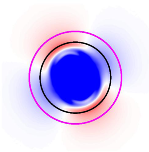
Figures 7(a,b) show the vorticity distributions at  $t=0$ and several days later for an anticyclone (bounded by the black circumference) over a narrow Gaussian mountain (magenta circumference). The vorticity profile is shown in figure 2(b). The results indicate that the disturbance grows and misaligns the vortex core from the origin. Hence the characteristic wavenumber is $k_c = 1$, which agrees with that predicted by the spectral method (black curve in figure 6a). The new structure can be characterised as an asymmetric dipolar vortex trapped over the mountain, as discussed in Gonzalez & Zavala Sansón (Reference Gonzalez and Zavala Sansón2021). To verify that the fastest growing mode has $k_c=1$, we calculate the time evolution of the perturbations amplitude as done by Carton & Legras (Reference Carton and Legras1994). First, the vorticity perturbation is defined as
 \begin{equation} \omega'(r,\theta,t)=\omega(r,\theta,t)-\nabla^2\varPsi(r). \end{equation}
Second, this field is decomposed in angular modes
 \begin{equation} \{C_k(r,t),S_k(r,t)\}=\frac{1}{\rm \pi}\int_0^{2{\rm \pi}} \omega'(r,\theta,t)\,\{\cos(k\theta), \sin(k\theta) \}\,{\rm d}\theta, \end{equation}
whose amplitudes are
 \begin{equation} A_k(t) =\frac{1}{r_{max}}\int_0^{r_{max}}[C_k^2(r,t) + S_k^2(r,t)]\, {\rm d} r, \end{equation}
with  $r_{max}\sim 4s_l$. Figure 7(c) presents the amplitudes time evolution for modes $k=1- 5$. After a brief initial period of adjustment, the amplitudes remain small and constant during 120 days, approximately. Afterwards, amplitude $A_1$ grows faster than the others, in agreement with the prediction of the stability analysis.

Figure 7. Numerically calculated vorticity distributions of an anticyclone over a narrow mountain  $(\xi _t,s_t)=(1,2)$ at (a) $t = 0$ days, and (b) $t= 160$ days. The limits of the colour bars are set by the peak vorticity $\omega _{min}=\min \{\omega _a\}$. (c) Time evolution of five azimuthal mode amplitudes $A_k$ (see text). The fastest growth is for $k=1$.
Figures 8(a) and 8(b) presents the vorticity distributions for an anticyclone over a wide Gaussian mountain (the vorticity profile is shown in figure 2d). Note that the external ring of positive vorticity is very weak in comparison to the anticyclonic centre. The simulation indicates that the anticyclonic core is displaced from the origin, yielding a weak dipolar structure over the topography. This result agrees with the corresponding instability profile in figure 6(b) (black curve), which predicts that the fastest growing mode has a characteristic wavenumber  $k_c = 1$ for this configuration. The dipole-like vortices emerging from this and the previous simulation have very different structures because of the radical differences in their initial vorticity profiles. Figure 8(c) presents the perturbations amplitude evolution, where it is verified that the most unstable mode is $k_c = 1$.

Figure 8. Numerically calculated vorticity distributions of an anticyclone over a wide mountain  $(\xi _t,s_t)=(1,5)$ at (a) $t = 0$ days, and (b) $t= 143$ days. (c) Time evolution of five azimuthal mode amplitudes $A_k$. The fastest growth is for $k=1$.
In figure 9, we present a case similar to that shown in figure 8, but now with  $\xi _t = 3$ (a higher mountain or weaker vortex). In this case, the dominant mode has wavenumber $2$, yielding an anticyclonic core with two positive vorticity satellites. The spectral solution also points out that the characteristic wavenumber is $k_c = 2$ (see the blue curve in figure 6b). The vortex evolution during an extended period is shown in supplementary movie 1, available at https://doi.org/10.1017/jfm.2023.153. The structure rotates as a whole in the clockwise direction around the mountain. This new vortex resembles the well-known tripolar vortices observed in laboratory experiments, which have a cyclonic core and two negative satellites, and rotate anticlockwise (Kloosterziel & van Heijst Reference Kloosterziel and van Heijst1991). However, the vorticity distribution is notoriously different to the typical tripoles because here the core is anticyclonic, and the cyclonic satellites are very weak. Furthermore, the vortex motion is affected by the topography. The amplitudes shown in figure 9(c) verify that the most unstable mode is $k_c=2$.

Figure 9. Numerically calculated vorticity distributions of an anticyclone over a wide mountain  $(\xi _t,s_t)=(3,5)$ at (a) $t = 0$ days, and (b) $t= 500$ days. (c) Time evolution of five azimuthal mode amplitudes $A_k$. The fastest growth is for $k=2$.
Overall, the numerical experiments indicate that most of the A/M and C/V configurations are unstable. We performed additional simulations for C/M and A/V cases, which showed that the initial vorticity distributions remained stable during very long time integrations in all cases. As an example, the evolution of a cyclone over a mountain (with  $s_t=2$, $\xi _t=-4$) during an extended period is shown in supplementary movie 2. These results are in agreement with the stability analysis, which yields a zero growth rate in these configurations, and also with the barotropic instability theorems found in §§ 3.2 and 3.3 because the necessary instability criteria are not met.
Table 2 compares the wavenumber of the fastest growing mode calculated from the eigenvalue problem and that observed in the numerical simulations. We consider narrow and wide topographies with  $1\le \xi _t\le 4$ (A/M or C/V) and $-4\le \xi _t\le -1$ (C/M or A/V). In almost all configurations, the wavenumber obtained with both methods is the same, which suggests that the linear analysis provides reliable results. However, there are a few discrepancies, such as the two configurations with $\xi _t=3,4$ and $s_t=2$ (A/M or C/V over narrow topography). The instability analysis predicts $k_c=1$ and 2, respectively, but the numerically calculated vortices remained stable during about 600 days of simulation. The reason may be due to the small growth rate of the perturbation, as observed in figure 6(a). Probably, more simulation days would be necessary to appreciate the expected instability. Another discrepancy is the configuration with $\xi _t=2$ and $s_t=5$ (A/M or C/V over a wide topography), for which the predicted wavenumber is $k_c=1$ but the simulated vortex indicates $k_c=2$. In this case, the difference may be due to the almost equal growth rate values for both wavenumbers, as shown in figure 6(b) (light grey curve).
Table 2. Comparison of the characteristic wavenumber  $k_c$ predicted by the spectral solution of the generalised eigenvalue problem (§ 3.5) and that found in the numerical simulations for different vortex/topography configurations $(\xi _t,s_t)$.

4. Discussion and conclusions
We investigated the stability of cyclonic and anticyclonic circular vortices over isolated topographies, which can be either mountains or valleys. The results include: (i) a linear stability analysis that led to the generalised eigenvalue problem and to the incorporation of finite topography effects in classical instability theorems in the SW dynamics (§ 2); and (ii) the application of these results to QG analytical vortices over low-amplitude topography (§ 3). The latter analysis includes the spectral solution of the eigenvalue problem, and numerical simulations showing the long-term evolution of the vortices.
As a basic flow in § 3, we considered stationary, nonlinear analytical vortices over a Gaussian topography (Gonzalez & Zavala Sansón Reference Gonzalez and Zavala Sansón2021). The flow/topography configurations are characterised by the dimensionless number  $\xi _t$, which is the ratio between the relative height of the topography (whose sign indicates whether it is a mountain or a valley) and the Rossby number (also signed to distinguish cyclones and anticyclones). Thus the two dynamical configurations are comprised in cases with $\xi _t>0$ (A/M and C/V), and $\xi _t<0$ (A/V and C/M). The flat-bottom case is $\xi _t=0$. A second parameter is the horizontal scale of the topography $s_t$.
According to the spectral solution of the generalised eigenvalue problem, the configurations A/M and C/V are unstable. The characteristic wavenumbers of the fastest growing modes are  $k_c = 1$ and 2 in the range $1\le \xi _t\le 10$. The largest growth rates were found for smaller $\xi _t$ (figure 6), which indicates that the intense vortices are more unstable. In contrast, the growth rate is very small for $\xi _t\ge 3$ with narrow topography, and also for $\xi _t\ge 7$ with wide topography. This is an indication that the height of the topography may be a stabilising factor in these $\xi _t$ ranges. On the other hand, configurations A/V and C/M ( $\xi _t<0$) are linearly stable in all cases. These results agree with the analytical and numerical study of Zhao et al. (Reference Zhao, Chieusse-Gérard and Flierl2019) for the case of a Rankine vortex over a cylindrical mountain, which concluded that anticyclones are destabilised by seamounts while they are stabilised by depressions. Recently, numerical simulations carried out by Solodoch, Stewart & McWilliams (Reference Solodoch, Stewart and McWilliams2021) showed the formation and persistence of anticyclonic eddies over topographic depressions under a wide range of parameters, which is in agreement with the present result regarding the stability of the A/V configuration.
Long-term numerical simulations of vortices over topography agree well with the conclusions obtained from the eigenvalue problem. An aspect that stands out is that the new vortical structures emerging from unstable cases remain trapped and rotating around the topography. This behaviour resembles the asymmetric dipolar solutions obtained in Gonzalez & Zavala Sansón (Reference Gonzalez and Zavala Sansón2021), which rotate steadily around a seamount or valley. In Zavala Sansón & Gonzalez (Reference Zavala Sansón and Gonzalez2021), we reported that the residual flow over a submarine mountain after the passage of a travelling vortex is a dipolar structure that remains trapped around the tip of the mountain. A similar structure was found in laboratory experiments in a large rotating tank (Zavala Sansón et al. Reference Zavala Sansón, Barbosa Aguiar and van Heijst2012).
Let us discuss the stability properties in terms of the vorticity profiles of the different vortex solutions used here. In general, the vortices have non-zero circulation,  $\varGamma \ne 0$. For cases with $\xi _t > 0$ (A/M and C/V), the vorticity profiles have a core shielded by a ring with opposite vorticity (figure 2). We found that the potential vorticity gradient is zero somewhere (figure 4), so the vortices meet the modified Rayleigh and Fjørtoft instability criteria (2.15) and (2.20), respectively. Shielded vortices with $\varGamma =0$ on a flat bottom are also barotropically unstable (Carton & McWilliams Reference Carton and McWilliams1989; Kloosterziel & van Heijst Reference Kloosterziel and van Heijst1991). However, in the present cases with topography and $\varGamma \ne 0$, the external ring can have much more or much less vorticity than the vortex core. As a result, the emerging ‘tripolar’ vortex may have a very different aspect in comparison to the traditional, flat-bottom tripoles. An example with a very weak external ring was presented in figure 9.
For cases with  $\xi _t < 0$ (C/M and A/V), the vorticity profiles have definite sign, as shown in figure 3. The vorticity maximum might be either at the centre (unshielded monopoles) or at a certain radius off the origin (unshielded annuli, a vortex class that has been studied rarely). It was found that in all cases, the vorticity profiles do not meet the instability criteria, so the vortices are sufficiently stable. This result is in agreement with the well-known stable behaviour of unshielded, circular vortices found typically in laboratory experiments (Kloosterziel & van Heijst Reference Kloosterziel and van Heijst1992). However, the stable evolution over topography contrasts with that observed for a flat bottom by Carton & McWilliams (Reference Carton and McWilliams1989), who indicated that unshielded annuli with non-zero circulation exhibit a breaking behaviour.
Finally, we discussed centrifugal instability in the presence of topography, which can be contrasted with that obtained by Kloosterziel & van Heijst (Reference Kloosterziel and van Heijst1991) for rotating flows over a flat bottom. The new criterion depends on the second radial derivative of the topographic profile and is weighted by the factor  $\varDelta (L_D/L)^2$; see (2.34). Roughly, we found that cyclones tend to be centrifugally stable and anticyclones unstable when seated on mountains or valleys (figure 5). Laboratory experiments or additional three-dimensional simulations would be required to test these predictions.
Supplementary movies
Supplementary movies are available at https://doi.org/10.1017/jfm.2023.153.
Acknowledgements
Comments and helpful indications from the anonymous reviewers are gratefully acknowledged. In particular, suggestions from one reviewer led us to the formulation of the instability criteria for shallow-water flows.
Funding
J.F.G. thanks the Consejo Nacional de Ciencia y Tecnología (CONACYT, México) and the Secretaría de Educación de Bogotá (Colombia) for their support.
Declaration of interests
The authors report no conflict of interest.
Appendix A. Exterior field coefficients
The coefficients of the solution (3.1) are given by
 \begin{equation} \left. \begin{array}{c} a_{0} = \dfrac{1}{4}\{ f_{00}(4+s_l^2) + [4s_lf_{01} + 2s_l^2 (\xi_t\,H(s_l) - f_{00})]\ln s_l - \xi_t\,H(s_l)\,s_l^2 \},\\ a_{1} =\dfrac{1}{2}s_l[s_l(f_{00} - \xi_t\,H(s_l)) - 2f_{01}],\\ a_{2} = \dfrac{1}{4}(\xi_t\,H(s_l) - f_{00}), \end{array}\right\} \end{equation}
where  $f_{00}$ and $f_{01}$ are
 \begin{equation} \left. \begin{array}{c} f_{00} = J_0(s_l) -\xi_t \left( \dfrac{\rm \pi}{2}\,I_2(s_l)\,J_0(s_l) - \dfrac{\rm \pi}{2}\,Y_0(s_l)\,I_1(s_l)\right), \\ f_{01} = \xi_t\,\dfrac{\rm \pi}{2}\,Y_1(s_l)\,I_1(s_l), \end{array}\right\} \end{equation}
and  $I_1(s_l)$ and $I_2(s_l)$ are integrals involving the topography:
 \begin{equation} I_1(s_l) = \int_0^{s_l} H(s')\,J_0(s')\,s'\, {\rm d} s', \quad I_2(s_l) = \int_0^{s_l} H(s')\,Y_0(s')\,s'\, {\rm d} s'. \end{equation}
Further details about these coefficients and the properties of the background flow can be consulted in Gonzalez & Zavala Sansón (Reference Gonzalez and Zavala Sansón2021).


