


1. Introduction
Mass loss from the Antarctic ice sheet will lead to a significant rise in the global sea level under the influence of climate warming (e.g. Rignot and others, Reference Rignot, Velicogna, Den Broeke, Monaghan and Lenaerts2011, Reference Rignot2019). The mass of the Antarctic ice sheet is currently decreasing (Gardner and others, Reference Gardner2018), and some ice shelves have suffered large-scale collapse and increased basal melting (e.g. Rignot and others, Reference Rignot, Jacobs, Mouginot and Scheuchl2013; Liu and others, Reference Liu2015; Hogg and others, Reference Hogg2017). The entire Antarctic ice sheet has contributed to a sea level rise of 14.0 ± 2.0 mm since 1979, including 4.4 ± 0.9 mm from East Antarctica, making this sector a major contributor to the overall loss of ice-sheet mass (Rignot and others, Reference Rignot2019).
Ice-sheet mass balance can be estimated using three remote-sensing methods: mass budget method, satellite altimetry and satellite gravimetry (e.g. Shepherd and others, Reference Shepherd2012; Sasgen and others, Reference Sasgen, Konrad, Helm and Grosfeld2019). Shepherd and others (Reference Shepherd2018) estimated the mass balance of the Antarctic ice sheet during 1992–2017 through the above three methods and found considerable uncertainty among these methods for East Antarctica; hence, further observations or improvements to observation methods are needed. The mass budget method relies on a surface mass balance (SMB) model. The uncertainty of satellite gravimeter estimates mainly comes from the Glacial Isostatic Adjustment contribution, whereas the satellite altimetry is subject to both deviations (Zhou and others, Reference Zhou2019); therefore, continental scales are essential for mass-balance observations. Observations of accumulation rates and firn densification processes can be used to validate and improve SMB estimates from regional climate models and coupled firn models, as well as capture behaviours at scales below the resolution of numerical models.
On-site ground observation methods, such as stakes in farms and lines, snow pits, snow micropens and firn/ice cores, can provide point measurements accumulation rate data with low spatial resolution (e.g. Eisen and others, Reference Eisen2008; Kameda and others, Reference Kameda, Motoyama, Fujita and Takahashi2008; Ding and others, Reference Ding2011; Shepherd and others, Reference Shepherd2012; Proksch and others, Reference Proksch, Löwe and Schneebeli2015), whereas airborne or vehicle-mounted ground-penetrating radar can continuously detect the internal structure of the ice sheet (Medley and others, Reference Medley2014).
Yang and others (Reference Yang2020) used frequency-modulated continuous wave (FMCW) radar observations of the internal reflecting horizons (IRHs) of the ice sheet to estimate the accumulation rate. The two-way travel time (TWTT) of the reflected signal is converted to depth with an accurate density measurement and then to the equivalent ice mass in order to estimate the accumulation between two reflectors. This process requires firn/ice cores along a transect to obtain the density–age–depth data of the IRHs on the vertical profile. Due to the existence of isochronous layers, the ages of IRHs can be obtained over hundreds of kilometres from ice cores (Eisen and others, Reference Eisen2008). The density of multiple firn cores should be averaged to obtain the regional representative density profile (Laepple and others, Reference Laepple2016). However, it is very difficult to drill a sufficient number of cores to obtain a representative sample of the depth–density relationship along the transect. Therefore, a method for obtaining a continuous density profile is very important for accurately estimating accumulation by radar data. Van den Broeke (Reference Van den Broeke2008) combined the firn densification empirical model of Herron and Langway (Reference Herron and Langway1980) with a regional climate model to simulate the depth–density relationship of the entire Antarctic ice sheet with a spatial resolution of 55 km. Although this method has been improved by Ligtenberg and others (Reference Ligtenberg, Helsen and Van den Broeke2011) to achieve a resolution of 27 km, this is still much lower than the radar resolution, and cannot be used to effectively improve the estimation accuracy of accumulation rates. Therefore, the direct inversion of the density profile by radar is useful for understanding small scale variations in accumulation rate.
The purpose of this study is to establish an inversion method for determining the ice sheet density within the upper 100 m of the ice sheet. By analysing FMCW monostatic reflection signals, a vertical profile of the density–depth relationship can be obtained that can be used to analyse the densification mechanism and improve the accuracy of radar estimation of accumulation (Herron and Langway, Reference Herron and Langway1980; Verfaillie and others, Reference Verfaillie2012). The theoretical basis is that the amplitude of the reflection signal is related to the permittivity, which depends on the density.
At present, the main method of inverting for ice-sheet density profiles from radar is based on the reflection travel times measured during common midpoint surveys. Then methods including Dix inversion (Dix, Reference Dix1955), semblance analysis (e.g. Booth and others, Reference Booth, Clark and Murray2010, Reference Booth, Clark and Murray2011), interferometry (Arthern and others, Reference Arthern, Corr, Gillet-Chaulet, Hawley and Morris2013) or IRH propagation time (e.g. Brown and others, Reference Brown2012) are used to estimate the reflector depth and wave speed, which can, in turn, be used to estimate the layer permittivity and converted to density. Drews and others (Reference Drews2016) also used a similar method to estimate the thickness and air content of the firn. However, few papers have obtained continuous inversion density profiles. This shortcoming may exist because the distance between the transmitting and receiving antennas needs to be constantly changed, which makes the data collection process cumbersome. When data acquisition and density inversion are performed on monostatic reflection signals, the vehicle or aircraft can be equipped with both transmitting and receiving antennas to efficiently obtain the internal structure and density profile of the ice sheet, which is essential for understanding accumulation rate variability and analysing the densification mechanism along hundreds of kilometres of radar lines.
At present, few papers use monostatic reflection signals to invert for the ice-sheet density profiles. Grima and others (Reference Grima, Blankenship, Young and Schroeder2014) used radar statistical reconnaissance to invert for the surface density of Thwaites Glacier. Srinivasamurthy and others (Reference Srinivasamurthy, Gogineni, Dawood and Kanagaratnam2005) inverted FMCW radar data for the density and thickness of Arctic sea ice. In contrast, the density profile of the Antarctic ice sheet increased exponentially (e.g. Cuffey and Paterson, Reference Cuffey and Paterson2010), showing completely different characteristics from sea ice. Therefore, a new inversion method is needed to estimate depth–density profiles from monostatic radar measurements over grounded ice.
In this study, the theoretical bases of the inversion method are described. Then, radar waveform simulation and inversion are performed for the high-resolution ice core data. In order to validate the inversion method, results are compared to measurements from four ice cores selected from regions with different topographic, climatic and densification characteristics. Finally, radar data taken from within 88 km of ice core DT401 are inverted to obtain a continuous density profile.
2. Radar theory and data
2.1 Data
2.1.1 Radar data
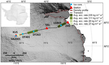
The 32nd Chinese National Antarctic Research Expedition (CHINARE) inland team surveyed the Antarctic ice sheet using FMCW radar (15–30 December 2015). The transect passed from Zhongshan Station through Taishan Station to Dome A, covering a total distance of 1280 km (black line in Fig. 1). The radar was mounted on a vehicle with antennas placed parallel to each other and separated by 2 m on the left side of the cabin. The vehicle moved at a constant speed of 14 km h−1 and the transmitter, receiver and controller performed continuous measurements.
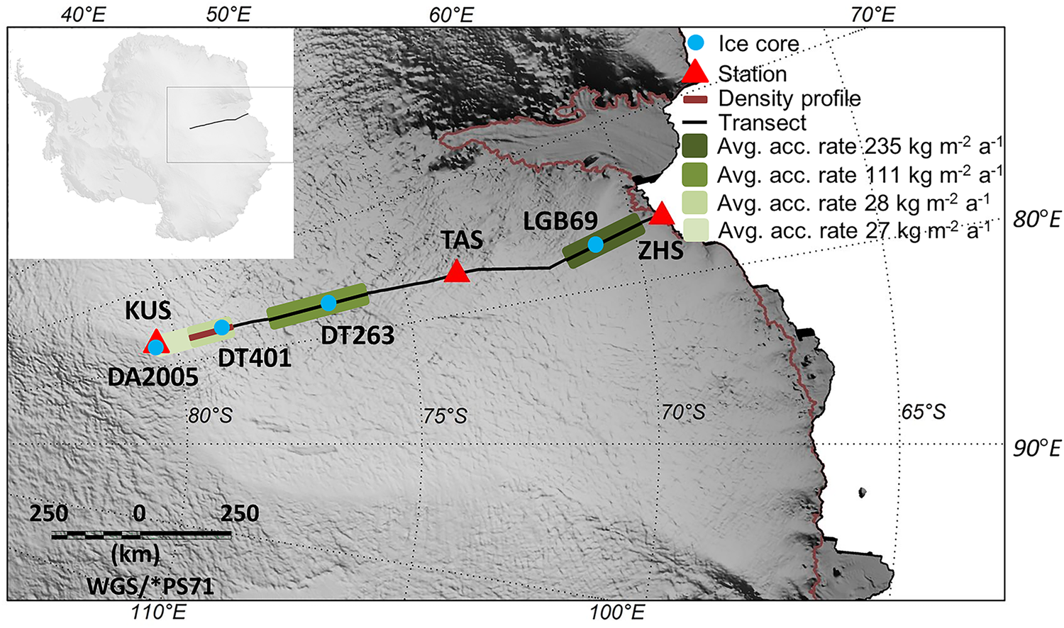
Fig. 1. Map of the radar traverse route from Zhongshan Station to Dome A shown by a black line. The blue dots indicate the positions of the ice cores (LGB69, DT263, DT401 and DA2005) used for the density inversion. The brown line indicates the 88 km density profile near ice core DT401, and the red triangles show the locations of Zhongshan Station (ZHS), Taishan Station (TAS) and Kunlun Station (KUS). The four green shades indicate the average accumulation rate (avg. acc. rate) from radar along the transect (Guo and others, Reference Guo2020).
A number of studies have shown that there are differences in the densification rate across East Antarctica regions, which are related to factors such as accumulation rate and temperature (e.g. Herron and Langway, Reference Herron and Langway1980; Van den Broeke, Reference Van den Broeke2008). To verify the applicability of the inversion algorithm, we selected four ice cores along the transect (LGB69, DT263, DT401 and DA2005 in Fig. 1), performed density inversion of the nearby radar data, and compared the results with the ice core density for error analysis. Finally, we estimated the continuous density distribution along an 88 km transect that crosses the location of ice core DT401 (brown line in Fig. 1) (Table 1).
Table 1. GPS, depth, elevation, drilling time, average temperature, average attenuation rate and references for density inversion of the ice cores

2.1.2 High-resolution density profile data
In order to verify the density inversion algorithm in this paper, we studied high-resolution density profiles of ten different locations (Table 2). These ice cores come from Greenland and the Antarctic Plateau regions and Antarctic coastal regions. The density is measured using a non-destructive logging system, and the measured intensity of the attenuated gamma-ray beam through the ice core is converted into a density signal. Wilhelms (Reference Wilhelms1996) gives the details and background of the method.
Table 2. Ten firn core sites with position, mean annual temperature, elevation and density characteristics

Note: RMSE and correlation: fitting result between densification rate and density std dev..
2.2 FMCW radar
The upper part of the Antarctic ice sheet is a mixture of air and ice called firn, where the density varies between 300 and 900 kg m−3. The path, electromagnetic field strength and waveform of electromagnetic waves vary with the dielectric properties and geometry of the medium, and reflections occur where the dielectric properties are discontinuous (Cui and others, Reference Cui2010). Dall and others (Reference Dall2010) did not find anisotropy within the upper 200 m of the ice sheet, so ice anisotropy is ignored in the density inversion algorithm. In this paper, the internal structure of the ice sheet is assumed to be parallel snow stratifications with different dielectric properties. The transmitting antenna produces an electromagnetic wave with a sweep period of 4 ms. The wave propagates vertically downwards, and part of the wave is reflected each time it passes through the interface between stratifications. These reflected signals are detected by the receiving antenna and combined with the reference signal generated by a voltage-controlled oscillator to generate a beat signal.
The time-domain beat signal is represented by the following formula (e.g. Srinivasamurthy and others, Reference Srinivasamurthy, Gogineni, Dawood and Kanagaratnam2005), and the parameters are presented in Table 3:


where f 0 represents the starting frequency (0.5 GHz), B represents the bandwidth (1.5 GHz) and t swp is the frequency sweep period of 4 ms. The amplitude of the reflection signal at the kth interface is related to the amount of attenuation A k, the reflection coefficient $\Gamma _k$ and the transmission coefficient T j of the jth layer above the kth interface; f k represents the frequency component of the kth interface reflection in the beat signal and φ k is the phase information, and it is not related to the initial phase of the transmitted signal (e.g. Stove and others, Reference Stove1992).
Table 3. Properties of beat signal and ice-sheet parameters

In view of the frequency sweep period, the bandwidth in the GHz range and f k in the kHz range, the second term in Eqn (2) can be omitted, and the phase difference δ k is ~180° (reflection from interface between high permittivity and low permittivity) or 0° (reflection from interface between low permittivity and high permittivity). The TWTT of the signal, τ k, is proportional to f k and can be expressed as follows:

Each frequency f k in the beat signal corresponds to a reflection from a subsurface interface. The determinant of the reflection interface in the beat signal is the frequency f k, which can be used to obtain the TWTT of the reflection interface by Eqn (3). The beat signal is sampled at a rate of 6.25 MS s−1 to obtain N = 25 000 samples. To reduce the spectrum leakage and improve the frequency resolution of spectrum transformation, the length of the beat signal is zero-padded to mN (additional (m − 1)N zeros, m integer), and then a fast Fourier transform (FFT) is performed (e.g. Okorn and others, Reference Okorn2014). The resulting spectrogram has many peaks (red line in Fig. 2), and each peak represents a reflection from an interface.
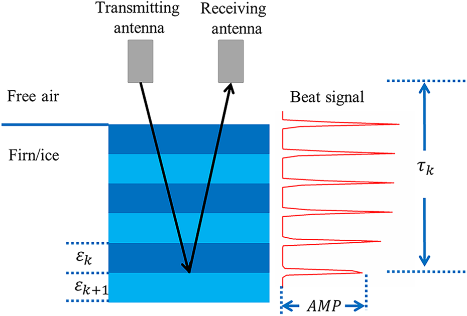
Fig. 2. Density is inverted from the amplitude (AMP) and TWTT (τ k) of the spectral peak of the beat signal. The spectrum amplitude of the beat signal is related to the permittivity difference between layers, and the permittivity depends on the density.
The location of the kth peak represents the TWTT from the antenna to the depth d k, and the amplitude AMP of the peak corresponds to the amount of attenuation A k and the transmission/reflection coefficient (Eqns (6), (7) and (11)). These parameters can be expressed by the following formulas:


where ɛ eff is the effective permittivity between the antenna and the kth interface and c represents the vacuum electromagnetic wave velocity. The definitions of the reflection coefficient $\Gamma _k$ and transmission coefficient T j are as follows (e.g. Okorn and others, Reference Okorn2014):


An analysis of Eqns (4–7) reveals that the amplitude of each peak in the beat signal spectrum is directly related to the dielectric behaviour between layers (ɛ k+1 and ɛ k). Landau and Lifschitz (Reference Landau and Lifschitz1982) addressed the dielectric behaviour of firn/ice in the form of a complex-valued relative permittivity ɛ in Eqn (8):

where the real part ɛ′ is the relative permittivity. Kovacs and others (Reference Kovacs, Gow and Morey1995) proposed an empirical formula between the density ρ (kg m−3) and the real permittivity ɛ′ as follows:

According to Fujita and others (Reference Fujita, Matsuoka, Ishida, Matsuoka, Mae and Takeo2000) and Matsuoka and others (Reference Matsuoka, Macgregor and Pattyn2010), the real part of the relative permittivity is also a function of the ice temperature, although it only causes a difference of <1%, which is much smaller than the crystal structure change during the densification process. Therefore, we do not consider the effect of temperature on the real part.
In this paper, we consider reflections in the upper 100 m of the ice sheet where density is the main cause of reflection, and the imaginary part can be ignored (i.e. Miners and others, Reference Miners1997, Reference Miners, Wolff, Moore, Jacobel and Hempel2002; Eisen and others, Reference Eisen, Wilhelms, Nixdorf and Miller2003; Arcone and others, Reference Arcone, Spikes, Hamilton and Mayewski2004). The density tends to be constant when below 200 m, although some layers in the ice sheet are rich in volcanic aerosols due to snowfall and volcanic eruptions, which will cause abrupt changes in the imaginary part ɛ′′ and generate reflections (Millar and others, Reference Millar1982). Since the imaginary part is much smaller than the real part in the upper 100 m, ice is a low-loss medium (Zirizzotti and others, Reference Zirizzotti, Cafarella, Urbini and Baskaradas2014). The attenuation constant α k and the amount of attenuation A k are given as follows (e.g. Ulaby and others, Reference Ulaby, Michielssen and Ravaioli2010):


Since ice is a non-magnetic material, the vacuum permeability is μ = 4π × 10−7 H m−1. Equation (10) shows that the attenuation constant α k depends on the conductivity.
Acidity and salinity have linear effects on conductivity (MacGregor and others, Reference MacGregor2007) and affect the attenuation constant. In coastal areas, wind carried salt from the ocean will increase the conductivity of the ice sheet with new snow accumulation, whereas the oceanic effect in inland areas (>100 km from the coast) can basically be ignored (Gow, Reference Gow1968). The study area in this paper is >160 km from the coast; therefore, we ignore the spatial variability of acidity and salinity along the transect.
Given the ~30°C surface temperature difference along the transect, we calculate the temperature-induced variation in conductivity (Table 1; MacGregor and others, Reference MacGregor2007; Zirizzotti and others, Reference Zirizzotti, Cafarella, Urbini and Baskaradas2014):

where E 0 = 0.33 ± 0.03 eV represents the mean activation energy (MacGregor and others, Reference MacGregor2007), k is Boltzmann's constant and T r is the temperature 258 K. Using Eqn (12), we can calculate the effect of temperature change on the attenuation rate. We find that there is a significant difference in the attenuation rate within the firn column (Table 1), so the attenuation coefficient must be corrected before inverting for density.
Since the available conductivity measurements along this transect are non-existent, we use the average conductivity (σ 0 = 23.16 μS m−1) of the DML cores B31, B32 and B33 collected by Oerter and others (Reference Oerter2000) with similar atmosphere and accumulation rate to calculate the attenuation coefficient. The conductivity must be recalibrated to the average temperature at each site in order to calculate the local attenuation rate, which is needed to compensate the radar power for attenuation losses.
In summary, we establish the density inversion algorithm based on the following assumptions: (1) the signal reflection is only caused by the permittivity difference, whereas conductivity differences in the vertical profile caused by snowfall and other sources (e.g. salt and ash) are ignored. (2) The conductivity is assumed to be constant and not a function of either depth or distance along the transect. (3) As an ice sheet is composed of layers of differing permittivity and birefringence (Fujita and others, Reference Fujita, Maeno and Matsuoka2006), we can simulate the FMCW radar reflections of upper 100 m ice sheets using horizontal layered structures (Eisen and others, Reference Eisen, Wilhelms, Nixdorf and Miller2003).
2.3 Radar processing
2.3.1 Radar trace processing
The amplitude of each peak in the beat signal spectrum has a direct relationship with the permittivity. The permittivity of the next layer ɛk+1 can be estimated by combining the reflected signal amplitude, the permittivity of the upper layer ɛk and Eqns (4, 6 and 7). When the surface permittivity of the ice sheet is known, we can extract the peak of the spectrum and obtain the permittivity along the entire vertical profile through continuous recursion and convert the permittivity to density using Eqn (9).
However, the peak of the radar record is not a reflection caused by the sudden change in permittivity; since the firn can be divided into many thin layers, the peaks are formed by the interference among many weak reflections caused by tiny permittivity differences (e.g. Harrison, Reference Harrison1973; Clough and others, Reference Clough1977). According to the high-resolution (5 mm) ice core data (Oerter and others, Reference Oerter2000), the density of adjacent thin layers also shows obvious differences in permittivity. Since the permittivity varies within the ice sheet, a reflected wave will be generated when the wave propagates from a low to high permittivity or a high to low permittivity layer, although the phase difference δ k (Eqn (2)) will differ by 180°. Okorn and others (Reference Okorn2014) proposed using δ k to determine whether the peak is caused by the permittivity increase or decrease. We found that the amplitude and phase is affected by spectrum leakage, which leads to uncertainty of δ k and incorrect permittivity trends. However, if we assume that density increases monotonically with depth, then the permittivity and hence density trend can be extracted from a smooth fit to the radar reflectivity, eliminating the influence of permittivity variability.
Since the permittivity contrast between air and firn massively exceeds the ice-sheet surface density variability (Grima and others, Reference Grima, Blankenship, Young and Schroeder2014), the maximum spectral peak amplitude at the surface is normalised to 1. According to Eqn (1), the amplitude generated by the ice-sheet surface only requires the reflection coefficient. Therefore, we use the surface density to estimate the reflection coefficient at the surface, which is used for inverse renormalised transformation, convert the amplitude of the radar record into the reflection coefficient that can be used to recursively invert the density profile.
2.3.2 Verification processing method
The radar trace actually reflects the std dev. of density within a given depth interval, rather than densification rate, where the latter is used to express the change of density with depth in this paper (Lewis and others, Reference Lewis2015). We have not found enough evidence to show a direct link between the density variability and the densification rate. However, both variables show similar patterns, that is, they rapidly decrease with depth, and this rate of change gradually slows with depth (Freitag and others, Reference Freitag, Wilhelms and Kipfstuhl2004; Hörhold and others, Reference Hörhold, Kipfstuhl, Wilhelms, Freitag and Frenzel2011). Therefore, we show that the two are correlated, and we fit and compare the ice core density std dev. with the average densification rate (the first derivative of density–depth relationship) across a moving average of 0.1 m to test this hypothesis.
Taking ice core B16 as an example, the densification rate and std dev. of the ice core density are normalised to [0,1] and fitted, which the fitting residual of the fourth-order polynomial function is the lowest. We used the same method to analyse the remaining ice cores, and the minimum residual function was used to fit the densification rate and the density std dev..
The root mean square error (RMSE) and correlation of the fitting results of the densification rate and the density density standard deviation is shown in Table 2, most of which have similar fitting results. The profiles present similar characteristics ‘cross-over’ (green and blue lines in Fig. 3a), which gradually decreasing with depth and increasing again in the middle of the firn column (Freitag and others, Reference Freitag, Wilhelms and Kipfstuhl2004). The cross-over characteristic of density variability leads to the lowest fitting residuals of fourth-order polynomials at most sites, but the exponential function has the lowest fitting residuals in B33 (red line in Fig. 3b).

Fig. 3. Densification rate and density std dev. of the ice core. (a) The densification rate and density density standard deviation of ice core B16 and the fourth-order polynomial fitting results and (b) the fitting densification rate and density density standard deviation of ice cores B21 and B33.
However, the green and blue lines in Figure 3a are not completely consistent: the densification rate is lower at 0–25 m and higher at 25–70 m. If we input the std dev. instead of the densification rate of ice core B16 into the density inversion algorithm in Section 3, the density above 25 m will be overestimated, but the error will decrease as the depth increases.
The average densification rate of B21 within the upper 30 m is only 0.18, which is much lower than the average density std dev. (0.34), resulting in an RMSE between the fitted densification rate and density std dev. of 52.2%, and the correlation is only 0.612. In Table 2, the RMSE of the ice cores except for B21 is within 20% and the correlation is >0.9, which can be used to judge whether the density std dev. is similar to the densification rate. According to the statistical data in Table 2, the density std dev. can be used as a proxy for the normalised densification rate in parts of Greenland and Antarctica. It is best to confirm the feasibility of this proxy in the study area through the above criteria before density inversion, and choose the polynomial or exponential function formula with the lowest residual for fitting.
3. Inversion
The density profile is obtained from the radar data by the following process:
1. Obtain the surface density and permittivity.
2. Convert the original radar data into a frequency spectrum by a zero-padded FFT; record the amplitude and TWTT of the spectrum peaks, which is fitted by the function with the smallest residual error (exponential or polynomial function).
3. Renormalise the fitted spectrum to the reflection coefficient profile, and record the reflection coefficient at the TWTT of each peak.
4. Calculate the average permittivity of the next layer from the reflection coefficient profile by Eqns (6–7, 11) and obtain the thickness of the layer by multiplying the TWTT between the peaks with the wave velocity of the next layer.
5. Recursively obtain the permittivity of the entire vertical section.
6. Convert the permittivity to density by Eqn (9).
4. Simulation, sensitivity tests and ice core inversion
Before analysing the FMCW radar data collected on a site in East Antarctica, we establish a theoretical model and verify the inversion algorithm through simulated radar data. Accounting for the change in density with depth, we input the ice core permittivity data with high depth resolution (5 mm) into the beat signal model and then perform the density inversion based on the generated waveform spectrum to verify the effectiveness of the inversion method.
4.1 Simulation
4.1.1 Modelling the radio-echo reflection
We will simulate the radar waveform at ice core LGB69 and compare it with the radar record to demonstrate that the beat signal simulation method is feasible. We model the ice sheet as a 1-D layered structure, the anisotropy of ice is ignored and only the variability of permittivity are considered.
The beat signal is simulated using Eqn (1) and the radar parameters in described in Section 2.2, including radar operating frequency (0.5–2 GHz), bandwidth (1.5 GHz) and sweep period (4 ms), and does not consider the characteristics of the radar system such as transmit power or antenna gain. For first-order simulations, layers are flat and stacked on top of one another (Leuschen, Reference Leuschen2001). We determine the reflection coefficient, transmission coefficient and attenuation of each interface according to the permittivity profile of the ice core LGB69 and use Eqn (5) to calculate the TWTT. The parameters are input into Eqn (1) to simulate the reflected signal of each interface and sum it to obtain the beat signal. Due to the lack of the permittivity measurements of ice core LGB69, we use Eqn (9) to estimate permittivity from the measured density. Therefore, we use cubic spline interpolation to improve the depth and permittivity sampling of LGB69. Finally, the permittivity profile and radar parameters are input into the simulator to generate beat signal time-domain waveforms. To perform a comparison with radar records, the simulated beat signal is also subjected to low-pass filtering and discrete sampling to simulate the influence of electronic equipment, and we use FFT to convert the simulated beat signal to the frequency domain.
We normalised the amplitude of the model and radar profile as shown in Figure 4. The ice core was drilled in 2001, and the radar detection time was 2015, and the 2001 surface was covered by ~5.02 ± 0.24 m in the 14 year period (Guo and others, Reference Guo2020). We choose the average surface density of 470 kg m−3 within 5 m of the ice core, and use Eqn (9) to estimate the average relative permittivity is 1.95, and the electromagnetic wave speed is ~0.21 m ns−1, so the TWTT in the increased snow is ~48 ns, and we remove the radar waveform in this range (Fig. 4b).

Fig. 4. Comparison of the beat signal simulation model and radar record. (a) Density profile of ice core LGB69; the pink dots are the measured density of the ice core and the black line is the cubic spline interpolation result. (b) Simulation frequency domain waveform (red line) based on the interpolated density; radar record around LGB69 (blue line). The radar records generated by the snowfall during the time period from the drilling of the ice core to the radar detection are excluded. Five green dashed lines are randomly selected to compare the peaks of the two beat signals, and the age of the layer is marked on the right (Li and others, Reference Li, Xiao, Sneed and Yan2012). (c) The frequency domain waveform of the shaded area in (b).
The features of the model and radar are similar, with many large-amplitude reflections occur at the top of the ice sheet (within the upper 10 m). The green dashed line in Figure 4b indicates several typical peaks that are dated, indicating that the beat signal simulation model can indeed reproduce the reflection inside the ice sheet via density and permittivity. However, the amplitude of some peaks is different (e.g. the layer formed by 1970 and 1941), and some sharp peaks in the radar record are not shown in the simulated track (e.g. 45–65 m). We believe that the reason is that the depth resolution of LGB69 is only 0.5 m, resulting in a relatively smooth density profile produced by cubic spline interpolation, and the actual ice core density fluctuates more severely, resulting in the underestimation of the peak amplitude. The underestimated amplitude will affect the inversion; therefore, we test our inversion algorithm against simulations from high-resolution ice core data to ensure that our method is robust against small-scale variability in the depth–density profile.
4.1.2 Density profile inversion algorithm
Hörhold and others (Reference Hörhold, Kipfstuhl, Wilhelms, Freitag and Frenzel2011) showed that the statistical microstructural properties and the densification of the density profiles in the regions where they collected ice cores in Antarctica are similar; therefore, we selected DML cores B31 and B33, which have similar temperature and accumulation conditions to those of ice core DT263, and DT263 is the ice core closest to the transect and was inverted in Section 4.3. We input the permittivity data of two DML cores (5 mm depth resolution) into the beat signal model to simulate the spectrum waveform for density inversion and analyse the influence of the spatial resolution, surface density and bandwidth on the inversion algorithm.
Using the different fitting functions (i.e. exponential or polynomial function), we build a 1-D layered model with a resolution of 5 mm based on the measured permittivity at ice cores B31 and B33 and use the method in Section 4.1.1 to simulate the beat signal, the lack of near-surface data for ice core B31 is set to the permittivity of the closest layer. The length of the signal is zero-padded to mN (m = 40; N = 25 000) using FFT, and the result is normalised as shown by the black line in Figures 5a, c.

Fig. 5. Simulated radar trajectory and density inversion results at ice cores B31 (a, b) and B33 (c, d). (a, c) The black line is the spectrogram of the beat signal model; red dots are peaks of the spectrum; the green line is the reflection coefficient of the ice core and the blue line is the fitting result of the peak. (b, d) Measured density (grey line), 1000-point moving average density profile (red line) and inversion density (blue line).
The fitting result with the minimum residual of the spectral peak is shown as the blue line in Figure 5. We input the ice core permittivity measurements to Eqn (6), and then smoothing the results using a 1 m moving average to calculate the reflection coefficient, and compare it with the fitted peaks. It is found that there is a correlation between them (the correlation coefficient of B31 is 0.83, and B33 is 0.97), which shows that it is feasible for the fitted radar trace peaks to represent the reflection coefficient. Because ice core B31 lacks a near-surface section of the original data, the correlation coefficient is reduced.
The fitted peak is directly related to the reflection coefficient, which depends on the density std dev. (Lewis and others, Reference Lewis2015). It can be seen from Section 2.2 that the density std dev. corresponds to the densification rate at ice cores B31 and B33. Therefore, the peak fitting function can be converted into an average reflection coefficient through the renormalisation of the surface reflection coefficient, and represent the densification rate for density inversion.
A polynomial and an exponential function are used to fit the peak of ice cores B31 and B33, respectively (blue line in Figs 5a, c). After discretisation, this value is combined with the average surface permittivity (1.61 at B31, 1.66 at B33) and the fitted peak to estimate the permittivity of the next layer through Eqns (4, 6 and 7); the permittivity along the entire vertical profile can be obtained through continuous recursion and converted to density by Eqn (9), resulting in RMSEs of 3.68% at B31 and 1.69% at B33 with the moving average ice core density of 5 m window. We believe that the larger error of ice core B31 is due to the incomplete permittivity data (within 5–10 m) published by Oerter and others (Reference Oerter2000).
4.2 Sensitivity test
4.2.1 Influence of small-scale fluctuations in density
To study the sensitivity of the inversion to the small-scale fluctuations in the density profile, we test a range of density profiles moving averaged using windows of size 0.07, 0.15 and 0.3 m, and invert the simulated radar trace for the density profile. The results are shown in Figure 6.
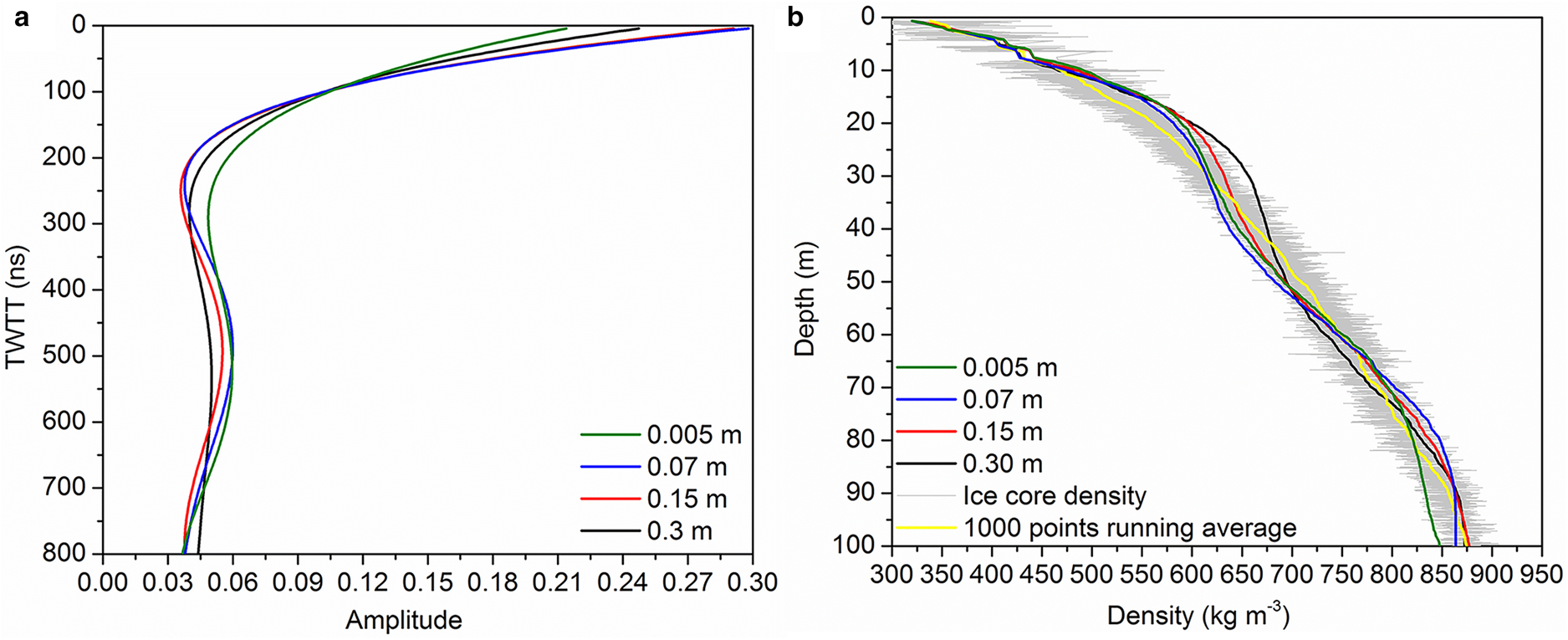
Fig. 6. Inverted density and peak fitting results of the original ice core data (green line) and the moving average of 0.07 m (blue line), 0.15 m (red line) and 0.3 m (black line). (a) The fitted spectral peak of the beat signal; (b) inverted density, ice core density (grey line) and 1000-point moving average density (yellow line).
A larger size of moving average window can reduce the std dev. and increase the depth of local minimum/maximum points without changing the average density. In the inversion algorithm, the spectrum is renormalised to the reflection coefficient and then recursively inverted to obtain the density profile, so the amplitude spectrum determines the densification rate. Since the frequency spectrum has been normalised in the inversion algorithm, so the absolute level difference between the beat signals can be eliminated. Therefore, the average amplitude of the 0.005–0.3 m window is similar (0.062, 0.060, 0.059 and 0.058, respectively), causing the inversion results of moving average at different depth intervals are similar.
The first local minimum point of the fitted peak of the 0.3 m window is deeper (black line in Fig. 6a), resulting in a higher densification rate between the ice-sheet surface and the local minimum point, and overestimating the inverted density within the upper 30 m.
The inversion algorithm is sensitive to small-scale fluctuations in the density profile, which will cause density errors at local depths, but still show the average density distribution along the vertical profile.
4.2.2 Influence of radar bandwidth
Radar bandwidth is an important factor related to resolution. Kanagaratnam and others (Reference Kanagaratnam, Gogineni, Gundestrup and Larsen2001) found that the FMCW radar has the strongest response in the 0.5–2 GHz frequency band, so we tested 0.3, 0.5, 0.8 and 1 GHz bandwidths to simulate the beat signal and invert for the density at ice core B31. The results are shown in Figure 7.

Fig. 7. Inverted density of 0.3 GHz (green line), 0.5 GHz (red line), 0.8 GHz (blue line) and 1 GHz (black line) bandwidths at ice core B31.
The depth resolution of the radar will decrease as the bandwidth decreases. And the bandwidth does not affect the depth of the local minimum/maximum of the density std dev., so the density inflection point does not shift compared with that shown in Figure 6b.
We found that due to the low radar resolution in the 0.3 GHz bandwidth, the local maximum/minimum in the spectrum cannot be distinguished, so the fitting residual of the exponential function is the smallest, resulting in a relatively smooth density profile without obvious inflection points, and the density near 60 m is overestimated.
The amplitude of the simulated radar traces varies with bandwidth. Although the density profiles in 0.5–1 GHz bandwidths are not completely consistent, the absolute level difference between the beat signals is eliminated by the normalisation in the inversion algorithm, and as a result, the inverted density still reflects the average density trend of ice core.
Based on the above simulation, we believe that the inversion method does not have strict bandwidth constraints, but the bandwidth alone can cause significant changes in the inverted profile. Therefore, it is necessary to be cautious when comparing the results of different radar systems, and choose the function with the smallest residual error to fit the peak of the spectrum.
4.2.3 Influence of surface density
The surface density or surface permittivity of the ice sheet is necessary for inversion and is the beginning of the recursion, which determines the inverted average density. To understand the sensitivity of the inversion to this parameter, we inverted the density profile in the surface density range between 280 and 380 kg m−3. The results are shown in Figure 8. The surface density strongly impacts the inverted density profile, but the densification profile (rate of change of density with depth) remains similar. Since Ding and others (Reference Ding2011) measured the surface density along the same transect used in this paper, we continue to use the measured surface density for inversion. However, it is clear that the quality absolute density measurements obtained by this method depend heavily on the reliability and representativeness of the surface density measurements to which they have normalised.
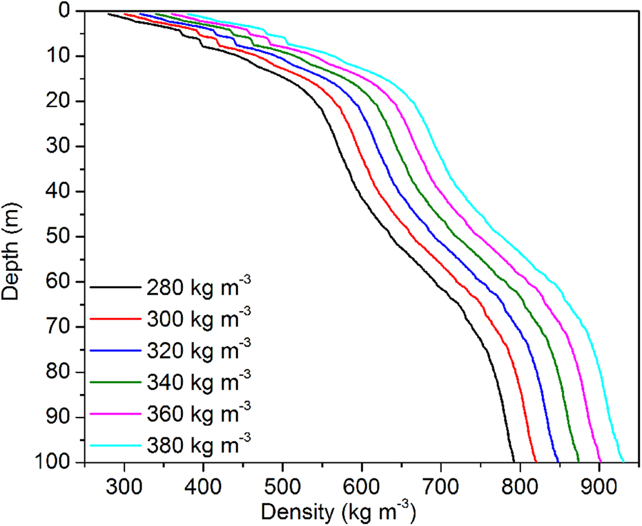
Fig. 8. Density inversion results using surface density of 280–380 kg m−3.
4.3 Density inversion around ice cores
The densification rates vary across the Antarctic ice sheet (e.g. Herron and Langway, Reference Herron and Langway1980; Van den Broeke, Reference Van den Broeke2008). In general, as the distance from the coast increases, the depth of the firn/ice transition increases and the surface density decreases (e.g. Van den Broeke, Reference Van den Broeke2008). This trend is related to factors such as the accumulation rate, redistribution of snow and surface temperature (e.g. Herron and Langway, Reference Herron and Langway1980; Van den Broeke, Reference Van den Broeke2008; Ligtenberg and others, Reference Ligtenberg, Helsen and Van den Broeke2011). Guo and others (Reference Guo2020) divided the transect from Zhongshan Station to Dome A into four areas based on the surface topography and meteorological characteristics. We selected ice cores from each area and compared the measured densities with the inversion results to evaluate the performance of the inversion method in this study.
The received signal has been amplified, mixed and sampled inside the radar system. Since we do not know the radar parameters such as transmit RF power, antenna gain, etc., it is difficult to directly calibrate the received power to the absolute level of the reflection coefficient. Therefore, the length of the signal is zero-padded to mN (m = 40) using FFT, and we normalise the spectrum to [0, 1]. As shown in Section 2.3, we use the ice core density to estimate the surface reflection coefficient of the ice sheet to renormalise the fitted spectral peak of the beat signal.
We performed coherent superposition and incoherent superposition in order to reduce the incoherent noise. After experimenting with the number of traces, we need to use at least 40 traces of data for coherent averaging. The density profile is unlikely to change suddenly over the course of densification, the radar data near ice core DA2005 are taken as an example; only the last trace among every ten traces is retained to reduce the data volume and calculation time, and test the effect of averaging between 40 and 200 traces. The theoretical maximum width of firn sampled by a trace can reach 0.278 m. The results show that the influence of width on the density RMSE is <1%, and a width of 180 traces (resolution: 0.278 × 180 × 10 = 500 m) produces the inversion with the least RMSE. Theoretically, the inversion result from a set of coherently averaged radar traces is the average density within 500 m (Arthern and others, Reference Arthern, Corr, Gillet-Chaulet, Hawley and Morris2013). Therefore, we select 500 m long segments radar data near the four ice cores to invert for the average density profile.
The above methods are used to invert the radar data near the four ice cores in Section 2.1 for density. The density profile (black line) and the densification rate (red and green line) are shown in Figure 9. The ice core density is fitted by smoothing spline and interpolated to increase the sampling. Finally, the densification rate of the ice core is obtained by calculating the first derivative of the density–depth relationship.

Fig. 9. Comparison of density profiles of ice cores LGB69 (a), DT263 (b), DT401 (c) and DA2005 (d) and inversion results. The blue dots are the ice core density, the black line is the density inversion result, the red line is the densification rate of the inverted density (first derivative of the density–depth relationship), the green line is the ice core densification rate and the grey dashed line is the inflection point of the density variability and the location of 830 kg m−3.
The firn/ice within the upper 100 m is divided into three areas according to the rate of change of density with depth, and these areas are separated by the grey lines in Figure 9. Herron and Langway (Reference Herron and Langway1980), Breton (Reference Breton2011) and Hörhold and others (Reference Hörhold, Kipfstuhl, Wilhelms, Freitag and Frenzel2011) used different division methods for the first area.
Herron and Langway (Reference Herron and Langway1980) and Breton (Reference Breton2011) reported that the first area (densification I) is between the ice-sheet surface and 550 kg m−3, whereas Hörhold and others (Reference Hörhold, Kipfstuhl, Wilhelms, Freitag and Frenzel2011) reported that it is between the surface and the density std dev. inflection point, which has a density of 600–650 kg m−3 (grey line in Fig. 9). The rapid compression of low-density layers results in the highest densification rate near surface of the ice sheet.
The second area (densification II) lies between the end of densification I and 830 kg m−3; here, the densification rate increases first and then decreases, and the main densification mechanism of the former is interparticle bond growth and particle deformation, whereas the latter is only particle deformation (Breton, Reference Breton2011).
The third area (densification III) is the area with density below 830 kg m−3, where the pores are closed off from the atmosphere and each other. The main densification factor in this zone is air pore compression, and the densification rate decreases rapidly (Herron and Langway, Reference Herron and Langway1980).
The critical density values of the four ice cores are shown in Table 4. They present similar characteristics: (1) we did not observe a sharp change in the densification rate at the density of 550 kg m−3; (2) the density–depth rate of change near the surface is high, with a rapid drop to a local minimum in the change rate at a density of 600–700 kg m−3, followed by a second relative maximum. The density of the inflection point in LGB69 and DT401 is greater than that of Hörhold and others (Reference Hörhold, Kipfstuhl, Wilhelms, Freitag and Frenzel2011) and (3) the firn/ice transition depth increases with the distance from the coast except in ice core DT401. The anomaly of DT401 is caused by the snow redistribution by wind, which will be discussed in detail in Section 5. These characteristics correspond to the conclusions of Hörhold and others (Reference Hörhold, Kipfstuhl, Wilhelms, Freitag and Frenzel2011), so we regard the inflection point as the end of the first densification zone.
Table 4. Critical values in the inversion density profiles for the ice cores

Note: First avg. densification rate: the average densification rate from the ice-sheet surface to inflection point in density std dev.; second avg. densification rate: the average densification rate at the depths between the inflection point in density std dev. and 830 kg m−3; and density RMSE: root mean square error between the inverted density and the ice core.
The inversion densification rate reflects the trend of the ice core density std dev., which decreases with depth and increases again in the middle of the firn column. And each ice core has unique regional characteristics, which are related to factors such as the accumulation rate, redistribution of snow and temperature (e.g. Herron and Langway, Reference Herron and Langway1980).
(1) LGB69: the difference between density std dev. and the densification rate may lead to the overestimation of density deeper than 60 m, and the densification rate of the ice core within 35–60 m only experienced a small increase far less than the inverted density, making the RMSE reach 2.24%. This ice core is located near the coast, resulting in a relatively high-accumulation rate (235 kg m−2 a−1; i.e. Fujita and others, Reference Fujita2011; Verfaillie and others, Reference Verfaillie2012); thus, the fresh snow is quickly buried and experienced higher overburden pressure, which increased the densification rate during the densification I stage (Ligtenberg and others, Reference Ligtenberg, Helsen and Van den Broeke2011). Moreover, firn sinters rapidly in densification II due to the relatively warm climate (Van Den Broeke, Reference Van den Broeke2008).
(2) DT263: the inversion result is consistent with the density characteristics and the inflection point depth of the ice core. The concavity of the densification profile flips between 47 and 65 m is completely opposite, the average inversion densification rate below the inflection point is 3.8 kg m−4, whereas that of the ice core is 4.0 kg m−4, resulting in a similar density–depth relationship between the inverted density and ice core. As noted in field surveys, the annual accumulation rate is low (111 kg m−2 a−1), a strong wind crust develops, and mass volatilisation occurs (Frezzotti and others, Reference Frezzotti2005; Ding and others, Reference Ding2011). The wind densifies the surface and the effect of grain settling is small (Sugiyama and others, Reference Sugiyama2012); as a result, the average densification rate in densification I is the lowest at only 5.92 kg m−4.
(3) DT401: the inversion result is similar to the trend of densification rate and the average densification rate (5.7 and 5.5 kg m−4, respectively) of the ice core, but the density RMSE is the highest due to the large variability in the ice core density. In the densification III stage, similar to the ice core density, the inverted density exceeds the theoretical pure ice density of 917 kg m−3 at depths >90 m (Qin and others, Reference Qin2000). Chemical species and solid dust particles may affect the structure, mechanical properties and sintering behaviour of ice, leading to a density increase.
(4) DA2005: this ice core is located in Dome A and shows good inversion results. This is one of the lowest accumulation rate regions in Antarctica, and the climate is cold (−58.5°C; Hou and others, Reference Hou, Li, Xiao and Ren2007), resulting in a relatively stable and slow densification process. The densification rate of the ice core does not have an obvious inflection point, and the inversion result reflects the densification process, and the RMSE is the smallest.
5. Density profile around Dome A
In Section 4, we mentioned that surface density measurements are needed to infer the surface reflection coefficient. The distance between ice cores DT401 and DA2005 is 150 km, and the reflection coefficient profiles obtained by renormalisation of the radar data are similar (std dev.: 2.8%), probably because both are high-altitude locations with low-accumulation rates. We use the surface reflection coefficient of DA2005 to begin the density inversion for DT401, which results in a density RMSE of <1%. Therefore, the surface properties of the two ice cores are similar, and we do not need continuous surface reflection coefficient data when inverting the continuous density profile between two ice cores, although this only holds where environmental conditions remain consistent.
Ding and others (Reference Ding2011) measured the vertical average density of the upper 0.2 m ice sheet along the same transect, which can be used for the density inversion of ice core DT401 and the transect 88 km to the southwest. The density profile within the upper 100 m obtained by inversion of radar data collected on this transect is shown in Figure 10.

Fig. 10. Comparison of the ice-sheet density profile, elevation (black line) and average accumulation rate (red line) within ice core DT401 and along radar transect 88 km to the southwest. (a) The green line is the position of ice core DT401, the black line is the critical density of 550 kg m−3 and the black dashed line is show the critical density of 830 kg m−3. (b) The average accumulation rate for 1350–2016 comes from Guo and others (Reference Guo2020); the blue line is the average densification rate from the ice-sheet surface to the depth of 830 kg m−3 along the transect.
Several studies have suggested that the critical densities of 550 kg m−3 and 830 kg m−3 can be used to analyse the densification process (e.g. Herron and Langway, Reference Herron and Langway1980), which are shown as black solid lines and black dotted lines in Figure 10a. We find that the trend of the depth of the 550 kg m−3 critical density is the same as that of the ice-sheet surface density along the transect, that is, deeper critical depth occurs with lower surface densities. The std dev. of the depth of the 830 kg m−3 critical density is 5.37 m, which is larger than that of 550 kg m−3 (1.04 m), so we focus on the depth variability of 830 kg m−3, which can more obviously reflect the trend of densification rate along the transect.
Guo and others (Reference Guo2020) divided the transect from Zhongshan Station to Dome A into four different regions, and the present study area falls within zone 3, which is 1080 km from the coast, with the highest elevation and one of the lowest accumulation rates in Antarctica (Ma and others, Reference Ma, Bian, Xiao, Allison and Zhou2010). The slope of zone 3 is steep, the elevation changes in the range of 3728–4000 m, with an average slope of 3.09 m km−1, and is affected by southwest winds (from right to left in Fig. 10). The strong katabatic winds redistribute snow, which leads to large fluctuations in accumulation rate, and affect the snow densification rate (Frezzotti and others, Reference Frezzotti2004; Ding and others, Reference Ding2011). The densification rate will increase with the accumulation rate (e.g. Lundin and others, Reference Lundin2017), which can be compared with the average densification rate from the ice-sheet surface to the depth of the 830 kg m−3 to verify the feasibility of the inversion algorithm. We believe that it is necessary to input parameters such as wind speed and surface slope to quantitatively analyse the spatial variability of the densification rate, but this is not the focus of this paper, so we only make a qualitative comparison here.
The densification rate and accumulation rate show a similar trend at the first 73 km transect in Figure 10b (correlation: 0.48). In general, the densification rate increases at the accumulation rate peak and decreases at the accumulation rate trough (e.g. ~4 and 6 km in Fig. 10b), which is consistent with Hörhold and others (Reference Hörhold, Kipfstuhl, Wilhelms, Freitag and Frenzel2011). This finding demonstrates that our density inversion retrieves profiles consistent with what we would expect from the physical conditions on the ice sheet.
The depth of the second critical density (830 kg m−3) significantly increases due to the proximity to Dome A (after 73 km), which is consistent with the climate models of Van den Broeke (Reference Van den Broeke2008) and Ligtenberg and others (Reference Ligtenberg, Helsen and Van den Broeke2011). We speculate that as the transect approaches Dome A, that is, closer to the ice divide, and the wind speed and the slope of the ice-sheet surface both drop, resulting in a lower densification rate (Fujita and others, Reference Fujita2015).
Guo and others (Reference Guo2020) reported the correlation between accumulation and surface topography in this region. We suggest that the spatial variability of the densification rate can also show a similar pattern; that is, the low densification rate typically occurs leeward of large slopes, and the high densification rate tends to appear downwind of surface depressions with relatively low slopes.
6. Conclusions
This paper describes a method for the inversion of ice-sheet density profiles using FMCW radar data. We first simulate and verify the inversion algorithm through the following four tests:
(1) The beat signal simulation model is compared with the radar record around ice core LGB69. The radar signal at ice core LGB69 is simulated, which shows that the reflection profile of the ice sheet can be reproduced using profiles of density and permittivity.
(2) The simulation and inversion of beat signals based on the high-resolution (5 mm) ice cores B31 and B33 show that it is feasible for the fitted radar trace peaks to represent the reflection coefficient. Therefore, we propose a renormalisation method based on the surface reflection coefficient to convert the fitted peak into an average reflection coefficient and represent the densification rate for density inversion.
(3) To study the sensitivity of the inversion method to radar bandwidth and small-scale density variability, we use the moving average of the ice core permittivity and different bandwidths to simulate beat signal and inversion density, and we obtain a similar density–depth relationship.
(4) We show that the surface density is a necessary prior parameter for the inversion, and is the beginning of the recursion, which determines the inverted average density.
The depth–density relationship is related to factors such as the accumulation rate, temperature and wind. Therefore, four ice cores from regions with different climate characteristics were selected along the transect from Zhongshan Station to Dome A, and the closest 500 m of radar data was used to validate the density inversion.
The average densities of the areas around the four ice cores were inverted by radar, and the density profiles were divided into three sections by inflection points in the densification rates which seem to correspond strongly with different modes of densification. Due to the warm climate and high-accumulation rate, the densification rate is high in ice core LGB69. Due to the influence of the wind crust and mass volatilisation around ice core DT263, grain settling is not obvious, resulting in the smallest average densification rate. The RMSE is the largest in ice core DT401 due to the fluctuation in the measured density. Ice core DA2005 at Dome A has a stable and slow compaction process.
We also analysed the radar data in the area with a low temperature and low-accumulation rate within 88 km southwest of DT401 and found that the strong katabatic winds erode the snow, causing snow redistribution, which leads to large fluctuations in the accumulation rate and densification rate along the transect. Moreover, the densification rate increases at the accumulation rate peak but decreases at the accumulation rate trough.
The entire inversion process is dependent on the surface density, surface reflection coefficient and the correlation between density std dev. and densification rate. A representative snow core can meet the demand of reflection coefficients within at least 150 km for the specific region we analysed. The radar density inversion method can achieve better results at high altitudes and low-accumulation rate areas. A small amount of liquid water will cause strong reflections and signal attenuation; therefore, it is difficult to perform this inversion in wet snow zones. The size and distribution of the percolation zone are annually transient in Antarctica and some high-altitude areas of Greenland (Brown and others, Reference Brown2012). The infiltration and refreezing of surface meltwater into the snow layer will cause a temporary increase in ice-sheet density variability and average density, which is not a severe concern in most of East Antarctica, although it cannot be ignored on the Greenland coast.
The maximum inversion RMSE of the four ice cores is 5.54%, which is similar to the accuracy of the common midpoint method (5%, Brown and others, Reference Brown2012; 6%, Arthern and others, Reference Arthern, Corr, Gillet-Chaulet, Hawley and Morris2013). It is best to confirm the correlation between the density std dev. and the densification rate before density inversion, which limits the study area of the inversion algorithm, but the obvious advantage is the efficient data collection process. Data extraction, analysis, inversion and imaging operations do not require manual intervention; therefore, a corresponding data analysis system can be established to automatically process the dataset.
The inverted density can be combined with the densification model (e.g. Herron and Langway, Reference Herron and Langway1980; Arthern and others, Reference Arthern, Vaughan, Rankin, Mulvaney and Thomas2010) to estimate the expected shape of the depth density distribution to further constrain the inversion results. With the introduction of radar parameters to the simulation, the received power can be calibrated to an absolute level for echo power comparison to invert the reflection coefficient for the density of the ice-sheet surface. In the modelling process, the anisotropy of ice is not considered; therefore, more factors can be considered to build a more complex inversion algorithm and fully utilise the information contained in the monostatic reflection signals.
After the algorithm is improved in future research, all radar data from Zhongshan Station to Dome A will be inverted to analyse the spatial variability of compaction along the transect. This study can be combined with on-site observations to further study the densification mechanism and effectively improve the estimation accuracy of accumulation rates from radar (Yang and others, Reference Yang2020). By analysing airborne FMCW radar data, continuous profiles of density and IRHs can be generated for hundreds of kilometres, which can improve our understanding of local accumulation rate variability.
Data
All the data presented in the paper are available for scientific purposes upon request to the corresponding author (douyk8888cn@126.com).
Acknowledgements
This study was funded by the National Natural Science Foundation of China (41776199, 41776204, 41876227, 41876230 and 41941006) and the National Key R&D Program of China (2018YFB1307504). The fieldwork was supported by the 32nd Chinese National Antarctic Research Expedition, especially the inland expedition team. We also thank the anonymous reviewers for many helpful edits and comments.
Author contributions
Y. Dou supervised the project. W. Yang, G. Zuo and Y. Wang conducted the fieldwork and processed the data under Y. Dou's supervision. Y. Wang performed all calculations and wrote most of the paper. B. Zhao, J. Guo and X. Tang studied the densification mechanism. Y. Chen and Y. Zhang provided the calculation method of the FFT. All authors contributed to the development of the analyses, interpretation of the results and extensive editing of the manuscript.


 Open access