2. Theoretical framework based on two-point Navier–Stokes equations

Interscale turbulence transfers for incompressible turbulence can be studied in the presence of all other co-existing turbulence transfer/transport mechanisms in terms of two-point equations exactly derived from the incompressible Navier–Stokes equations (see Hill Reference Hill2001, Reference Hill2002; Germano Reference Germano2007) without any hypotheses or assumptions, in particular no assumptions of homogeneity or periodicity. The incompressible Navier–Stokes equation is written at two points $\boldsymbol {\zeta } ^- =\boldsymbol {X}-\boldsymbol {r}$ and $\boldsymbol {\zeta ^+} =\boldsymbol {X}+\boldsymbol {r}$ in physical space (see figure 1), where $\boldsymbol {X}$ is the centroid and $\boldsymbol {2r}$ is the two-point separation vector. One defines the two-point velocity half-difference $\boldsymbol {\delta }\boldsymbol {u}(\boldsymbol {X},\boldsymbol {r},t)\equiv ({\boldsymbol {u}^+-\boldsymbol {u}^{-}})/{2}$, where $\boldsymbol {u}^+ \equiv \boldsymbol {u}(\boldsymbol {\zeta ^+})$ and $\boldsymbol {u}^{-} \equiv \boldsymbol {u}(\boldsymbol {\zeta ^-})$ are the fluid velocities at each of the two points, and the two-point pressure half-difference $\delta p (\boldsymbol {X},\boldsymbol {r},t) \equiv ({p^+- p^{-}})/{2}$, where $p^+ \equiv p(\boldsymbol {\zeta ^+})$ and $p^{-} \equiv p (\boldsymbol {\zeta ^-})$ are the pressure over density ratios at each of the two points. Incompressibility immediately imposes $\boldsymbol {\nabla _X}\boldsymbol {\cdot }\boldsymbol {\delta }\boldsymbol {u}=\boldsymbol {\nabla _r}\boldsymbol {\cdot }\boldsymbol {\delta } \boldsymbol {u}=0$ and the Navier–Stokes equation implies (Hill Reference Hill2001, Reference Hill2002)

(2.1)\begin{equation} \frac{\partial \boldsymbol{\delta} \boldsymbol{u}}{\partial t} + \left(\boldsymbol{u}_{\boldsymbol{X}}\boldsymbol{\cdot} \boldsymbol{\nabla}_{\boldsymbol{X}} \right) \boldsymbol{\delta} \boldsymbol{u} + \left(\boldsymbol{\delta}\boldsymbol{u}\boldsymbol{\cdot} \boldsymbol{\nabla}_{\boldsymbol{r}} \right) \boldsymbol{\delta}\boldsymbol{u} ={-}\boldsymbol{\nabla}_{\boldsymbol{X}} \delta p + \frac{\nu}{2}{\boldsymbol{\nabla}_{\boldsymbol{X}}}^2 \boldsymbol{\delta}\boldsymbol{u} +\frac{\nu}{2} {\boldsymbol{\nabla}_{\boldsymbol{r}}}^2 \boldsymbol{\delta}\boldsymbol{u}, \end{equation}

where $\boldsymbol {u_X} (\boldsymbol {X},\boldsymbol {r},t)\equiv ({\boldsymbol {u}^+ + \boldsymbol {u}^{-}})/{2}$; $\boldsymbol {\nabla }_{\boldsymbol {X}}$ and ${\boldsymbol {\nabla }_{\boldsymbol {X}}}^2$ are the gradient and Laplacian in $\boldsymbol {X}$ space; $\boldsymbol {\nabla }_{\boldsymbol {r}}$ and ${\boldsymbol {\nabla }_{\boldsymbol {r}}}^2$ are the gradient and Laplacian in $\boldsymbol {r}$ space; and $\nu$ is the kinematic viscosity.

Figure 1. Schematic of fluid velocities at points $\boldsymbol {\zeta } ^- =\boldsymbol {X}-\boldsymbol {r}$ and $\boldsymbol {\zeta ^+} =\boldsymbol {X}+\boldsymbol {r}$.

An energy equation is readily obtained by multiplying (2.1) with $2\boldsymbol {\delta }\boldsymbol {u}$:

(2.2)\begin{align} &\frac{\partial |\boldsymbol{\delta}\boldsymbol{u}|^2}{\partial t} + \boldsymbol{\nabla}_{\boldsymbol{X}}\boldsymbol{\cdot}(\boldsymbol{u_X} |\boldsymbol{\delta}\boldsymbol{u}|^2 ) + \boldsymbol{\nabla_r}\boldsymbol{\cdot}(\boldsymbol{\delta}\boldsymbol{u} |\boldsymbol{\delta} \boldsymbol{u}|^2 ) \nonumber\\ &\quad ={-} 2\boldsymbol{\nabla_X}\boldsymbol{\cdot}(\boldsymbol{\delta}\boldsymbol{u} \delta p) + \frac{\nu}{2}\boldsymbol{\nabla_X}^2 |\boldsymbol{\delta}\boldsymbol{u}|^2 + \frac{\nu}{2} \boldsymbol{\nabla_r}^2 |\boldsymbol{\delta}\boldsymbol{u}|^2 - \frac{1}{2}\epsilon^+- \frac{1}{2}\epsilon^-, \end{align}

where $\epsilon ^+ \,{=}\, \nu ({\partial u_i ^+}/{\partial \zeta ^+ _k})({\partial u_i ^+}/{\partial \zeta ^+ _k})$ and $\epsilon ^- \,{=}\, \nu ({\partial u_i ^-}/{\partial \zeta ^- _k})( {\partial u_i ^-}/{\partial \zeta ^- _k})$. With a Reynolds decomposition $\boldsymbol {\delta }\boldsymbol {u} =\overline {\boldsymbol {\delta }\boldsymbol {u}}+\boldsymbol {\delta }\boldsymbol {u}^{\prime }$, $\boldsymbol {u_X} = \overline {\boldsymbol {u_X}} + \boldsymbol {u_X}^{\prime }$, $\delta p = \delta \bar {p} + \delta p^{\prime }$ where the overline signifies an average over time under the assumption of statistical stationarity, this general two-point energy equation leads to the following pair of two-point energy equations:

(2.3)\begin{align} &\left(\overline{\boldsymbol{u_X}}\boldsymbol{\cdot}\boldsymbol{\nabla_X} +\boldsymbol{\delta}\boldsymbol{\bar{u}}\boldsymbol{\cdot}\boldsymbol{\nabla_r} \right)\frac{1}{2} |\boldsymbol{\delta}\boldsymbol{\bar{u}}|^2 + P_r + P_{Xr}^s + \frac{\partial}{\partial x_j} (\delta \overline{u_i}\overline{u_{Xj}^\prime\delta u_i^\prime}) + \frac{\partial}{\partial r_j} (\delta \overline{u_i}\overline{\delta u_j^\prime\delta u_i^\prime})\nonumber\\ &\quad={-} \boldsymbol{\nabla_X}\boldsymbol{\cdot}(\boldsymbol{\delta} \boldsymbol{\bar{u}}\delta \bar{p}) + \frac{\nu}{2}\boldsymbol{\nabla_X}^2 \frac{1}{2}|\boldsymbol{\delta} \boldsymbol{\bar{u}}|^2 +\frac{\nu}{2}\boldsymbol{\nabla_r}^2 \frac{1}{2}|\boldsymbol{\delta} \boldsymbol{\bar{u}}|^2 -\frac{\nu}{4} \frac{\partial \bar{u}_i ^+}{\partial \zeta ^+ _k} \frac{\partial \bar{u}_i ^+}{\partial \zeta ^+ _k} - \frac{\nu}{4} \frac{\partial \bar{u}_i^-} {\partial \zeta ^- _k} \frac{\partial \bar{u}_i ^-}{\partial \zeta ^- _k}, \end{align}

(2.4)\begin{align} &\left(\overline{\boldsymbol{u_X}}\boldsymbol{\cdot}\boldsymbol{\nabla_X} +\boldsymbol{\delta}\boldsymbol{\bar{u}}\boldsymbol{\cdot}\boldsymbol{\nabla_r} \right)\frac{1}{2} \overline{|\boldsymbol{\delta} \boldsymbol{u}^{\boldsymbol{\prime}}|^2} - P_r - P_{Xr}^s + \boldsymbol{\nabla_X}\boldsymbol{\cdot}\left(\overline{\boldsymbol{u_X}^\prime \frac{1}{2}|\boldsymbol{\delta} \boldsymbol{u}^\prime|^2}\right) + \boldsymbol{\nabla_r} \boldsymbol{\cdot}\left(\overline{\boldsymbol{\delta} \boldsymbol{u}^\prime \frac{1}{2}| \boldsymbol{\delta} \boldsymbol{u}^\prime|^2}\right) \nonumber\\ &\quad ={-} \boldsymbol{\nabla_X}\boldsymbol{\cdot}\overline{(\boldsymbol{\delta} \boldsymbol{u}^{\boldsymbol{\prime}} \delta p^\prime)} + \frac{\nu}{2}\boldsymbol{\nabla_X}^2 \frac{1}{2}\overline{|\boldsymbol{\delta} \boldsymbol{u}^{\boldsymbol{\prime}}|^2} +\frac{\nu}{2}\boldsymbol{\nabla_r}^2 \frac{1}{2}\overline{|\boldsymbol{\delta} \boldsymbol{u}^{\boldsymbol{\prime}}|^2} -\frac{\nu}{4} \overline{\frac{\partial u_i ^{\prime +}}{\partial \zeta ^+ _k} \frac{\partial u_i ^{\prime +}}{\partial \zeta ^+ _k}} - \frac{\nu}{4} \overline{\frac{\partial u_i ^{\prime -}}{\partial \zeta ^- _k} \frac{\partial u_i ^{\prime -}}{\partial \zeta ^- _k}} , \end{align}

where $P_r={-}\overline{\delta u_j ^\prime \delta u_i ^\prime}\frac{\partial \delta \overline{u_i}}{\partial r_j} ={-}\overline{\delta u_j ^\prime \delta u_i ^\prime}\frac{1}{2}[\varSigma_{ij}(\boldsymbol{X}+\boldsymbol{r}) + \varSigma_{ij} (\boldsymbol{X}-\boldsymbol{r})]$ and $P_{Xr}^s=-\overline {u_{Xj} ^\prime \delta u_i ^\prime } ({\partial \delta \overline {u_i}}/{\partial X_j})$, with $\varSigma _{ij} \equiv \frac {1}{2}({\partial \overline {u_i}}/{\partial X_j} + {\partial \overline {u_j}}/{\partial X_i})$, are two-point turbulence production rates. Indeed, being proportional to mean flow gradient terms and to averages of products of fluctuating velocities, they represent linear turbulence fluctuation processes and they exchange energy between $|\boldsymbol {\delta } \bar {\boldsymbol {u}}|^2$ and $\overline {|\boldsymbol {\delta } \boldsymbol {u}^{\boldsymbol {\prime }}|^2}$ because they appear with opposite signs in (2.3) and (2.4) as already noted by Alves Portela, Papadakis & Vassilicos (Reference Alves Portela, Papadakis and Vassilicos2017).

A complete two-point description also requires the evolution equation for the two-point velocity half-sum $\boldsymbol {u_X} (\boldsymbol {X},\boldsymbol {r},t)$. This equation was first obtained by Germano (Reference Germano2007):

(2.5)\begin{equation} \frac{\partial \boldsymbol{u_X}}{\partial t} + \left(\boldsymbol{u_X}\boldsymbol{\cdot}\boldsymbol{\nabla_X} \right) \boldsymbol{u_X} + \left(\boldsymbol{\delta} \boldsymbol{u}\boldsymbol{\cdot}\boldsymbol{\nabla_r} \right) \boldsymbol{u_X} ={-}\boldsymbol{\nabla_X} p_X + \frac{\nu}{2}\boldsymbol{\nabla_X}^2 \boldsymbol{u_X} +\frac{\nu}{2} \boldsymbol{\nabla_r} ^2 \boldsymbol{u_X}, \end{equation}

where $p_{X}\equiv ({p^++ p^{-}})/{2}$, and note that $\boldsymbol {u_X}$ is incompressible, i.e. $\boldsymbol {\nabla _X}\boldsymbol {\cdot }\boldsymbol {u_X}=\boldsymbol {\nabla _r}\boldsymbol {\cdot }\boldsymbol {u_X}=0$. An energy equation, also first derived by Germano (Reference Germano2007), is readily obtained by multiplying (2.5) with $2\boldsymbol {u_X}$:

(2.6)\begin{align} \frac{\partial |\boldsymbol{u_X}|^2}{\partial t} + \boldsymbol{\nabla_X}\boldsymbol{\cdot}(\boldsymbol{u_X} |\boldsymbol{u_X}|^2) + \boldsymbol{\nabla_r}\boldsymbol{\cdot}(\boldsymbol{\delta}\boldsymbol{u} |\boldsymbol{u_X}|^2) &={-} 2\boldsymbol{\nabla_X}\boldsymbol{\cdot}(\boldsymbol{u_X}p_X ) +\frac{\nu}{2} \boldsymbol{\nabla_X} ^2 |\boldsymbol{u_X}| ^2 \nonumber\\ &\quad + \frac{\nu}{2} \boldsymbol{\nabla_r} ^2 |\boldsymbol{u_X}| ^2-\frac{1}{2}\epsilon^+-\frac{1}{2}\epsilon^-. \end{align}

A pair of Reynolds-averaged two-point energy equations follows (using $p_{X} = \overline {p_X}+p_{X}^{\prime }$):

(2.7)\begin{align} &\left(\overline{\boldsymbol{u_X}}\boldsymbol{\cdot}\boldsymbol{\nabla_X} +\boldsymbol{\delta} \boldsymbol{\bar{u}}\boldsymbol{\cdot}\boldsymbol{\nabla_r} \right)\frac{1}{2} |\boldsymbol{\overline{u_X}}|^2 +P_X +P_{Xr}^l + \frac{\partial}{\partial x_j} (\overline{u_{Xi}}\overline{u_{Xi}^\prime u_{Xj}^\prime}) + \frac{\partial}{\partial r_j} (\overline{u_{Xi}}\overline{\delta u_j^\prime u_{Xi}^\prime})\nonumber\\ &\quad ={-} \boldsymbol{\nabla_X}\boldsymbol{\cdot}(\boldsymbol{\overline{u_X}} \overline{p_X}) + \frac{\nu}{2}\boldsymbol{\nabla_X}^2 \frac{1}{2} |\boldsymbol{\overline{u_X}}|^2 +\frac{\nu}{2}\boldsymbol{\nabla_r}^2 \frac{1}{2} |\boldsymbol{\overline{u_X}}|^2 -\frac{\nu}{4} \frac{\partial \bar{u}_i ^+}{\partial \zeta ^+ _k} \frac{\partial \bar{u}_i ^+}{\partial \zeta ^+ _k} - \frac{\nu}{4} \frac{\partial \bar{u}_i ^-}{\partial \zeta ^- _k} \frac{\partial \bar{u}_i ^-}{\partial \zeta ^- _k}, \end{align}

(2.8)\begin{align} &\left(\overline{\boldsymbol{u_X}}\boldsymbol{\cdot}\boldsymbol{\nabla_X} +\boldsymbol{\delta}\boldsymbol{\bar{u}}\boldsymbol{\cdot}\boldsymbol{\nabla_r} \right)\frac{1}{2}\overline{|\boldsymbol{u_X}^{\boldsymbol{\prime}}|^2} -P_X - P_{Xr}^l + \boldsymbol{\nabla_X}\boldsymbol{\cdot}\left(\overline{\boldsymbol{u_X}^\prime \frac{1}{2}|\boldsymbol{u_X}^\prime|^2}\right) + \boldsymbol{\nabla_r}\boldsymbol{\cdot}\left(\overline{\boldsymbol{\delta u}^\prime \frac{1}{2}| \boldsymbol{u_X}^\prime|^2}\right)\nonumber\\ &\quad ={-} \boldsymbol{\nabla_X}\boldsymbol{\cdot}(\overline{\boldsymbol{u_X}^\prime p_X^\prime}) + \frac{\nu}{2}\boldsymbol{\nabla_X}^2 \frac{1}{2}\overline{|\boldsymbol{u_X}^{\boldsymbol{\prime}}|^2} +\frac{\nu}{2}\boldsymbol{\nabla_r}^2 \frac{1}{2}\overline{|\boldsymbol{u_X}^{\boldsymbol{\prime}}|^2} -\frac{\nu}{4} \overline{\frac{\partial u_i ^{\prime +}}{\partial \zeta ^+ _k} \frac{\partial u_i ^{\prime +}}{\partial \zeta ^+ _k}} - \frac{\nu}{4} \overline{\frac{\partial u_i ^{\prime -}}{\partial \zeta ^- _k} \frac{\partial u_i ^{\prime -}}{\partial \zeta ^- _k}}, \end{align}

where $P_X={-}\overline{u_{Xj} ^\prime u_{Xi}^\prime}\frac{\partial \overline{u_{Xi}}}{\partial X_j} ={-}\overline{u_{Xj} ^\prime u_{Xi} ^\prime} \frac{1}{2}[\varSigma_{ij}(\boldsymbol{X}+\boldsymbol{r}) + \varSigma_{ij}(\boldsymbol{X}-\boldsymbol{r})]$ and $P_{Xr}^l=-\overline { \delta u_j ^\prime u_{Xi}^\prime } ({\partial \delta \overline {u_i}}/{\partial X_j})$. These two-point turbulence production rates represent linear turbulence fluctuation processes and an exchange of energy between $|\boldsymbol {\overline {u_X}}|^2$ and $\overline {|\boldsymbol {u_X^\prime }|^2}$ because they appear with opposite signs in (2.7) and (2.8).

Equations (2.3), (2.4) and (2.7), (2.8) offer a powerful and complete set of tools for the analysis of any turbulent flow and can be used to develop two-point turbulence theory and models which do not have to rely on homogeneity. In particular, (2.4) and (2.8) govern, respectively, the smaller-scale and the larger-scale fluctuating energy contributions to the total turbulent kinetic energy $\frac {1}{2} \overline {\vert \boldsymbol {u}^{\prime +}\vert ^{2}} + \frac {1}{2}\overline {\vert \boldsymbol {u}^{\prime -}\vert ^{2}}$. All physical processes are clearly represented: various turbulent production rates are present as already stated (and the total production rate $P_X + P_r + P_{Xr}^{s} + P_{Xr}^{l}$ transfers energy between $\frac {1}{2}\vert \bar {\boldsymbol {u}}^+\vert ^{2} + \frac {1}{2}\vert \bar {\boldsymbol {u}}^{-}\vert ^{2}$ and $\frac {1}{2} \overline {\vert \boldsymbol {u}^{\prime +}\vert ^{2}} + \frac {1}{2}\overline {\vert \boldsymbol {u}^{\prime +}\vert ^{2}}$); interspace turbulent transport and interscale turbulent transfer rates are represented by conservative terms in $\boldsymbol {X}$ and $\boldsymbol {r}$ spaces, respectively; pressure–velocity terms are also included as are viscous diffusion rates in both $\boldsymbol {X}$ and ${\boldsymbol {r}}$ spaces and turbulence dissipation rates. In the limit $\boldsymbol {r}\to \boldsymbol {0}$, $P_r$, $P_{Xr}^{s}$ and $P_{Xr}^{l}$ tend to $0$ and so do all the terms in (2.3) and (2.4) except the viscous diffusion and dissipation terms which balance by trivial mathematical identity at $\boldsymbol {r}=0$. However, $P_X$ tends to the one-point turbulence production rate in that limit, and (2.7) and (2.8) tend, respectively, to the one-point mean flow energy and the one-point turbulent kinetic energy equations at $\boldsymbol {X}$. For more details see Hill (Reference Hill2001, Reference Hill2002), Germano (Reference Germano2007) and Chen & Vassilicos (Reference Chen and Vassilicos2022).

3. Interscale turbulent energy transfers

Besides two-point turbulent production terms, the two-point energy equations of the previous section involve important interscale and interspace transport terms. Germano (Reference Germano2007) interpreted his (2.5) and (2.6) in the context of large-eddy simulations. He showed that the term $(\boldsymbol {\delta } \boldsymbol {u}\boldsymbol {\cdot }\boldsymbol {\nabla }_{\boldsymbol {r}}) \boldsymbol {u_X}$ in (2.5) can be interpreted as the gradient of a subgrid stress. This term gives rise to the term $\boldsymbol {\nabla _r}\boldsymbol {\cdot }(\boldsymbol {\delta } \boldsymbol {u} |\boldsymbol {u_X}|^2)$ in (2.6) which is therefore an energy transfer rate between large-scale velocities (velocity half-sum) and small-scale velocities (velocity half-difference). Germano (Reference Germano2007) also derived the kinematic equation

(3.1)\begin{equation} \boldsymbol{\nabla_r}\boldsymbol{\cdot}(\boldsymbol{\delta}\boldsymbol{u} |\boldsymbol{u_X}|^2) + \boldsymbol{\nabla_r}\boldsymbol{\cdot}(\boldsymbol{\delta}\boldsymbol{u} |\boldsymbol{\delta} \boldsymbol{u}|^2) = 2\boldsymbol{\nabla_X}\boldsymbol{\cdot}(\boldsymbol{\delta}\boldsymbol{u} (\boldsymbol{\delta} \boldsymbol{u} \boldsymbol{\cdot} \boldsymbol{u_X})) \end{equation}

which relates $\boldsymbol {\nabla _r}\boldsymbol {\cdot }(\boldsymbol {\delta } \boldsymbol {u} |\boldsymbol {u_X}|^2)$ to $\boldsymbol {\nabla _r}\boldsymbol {\cdot }(\boldsymbol {\delta } \boldsymbol {u} |\boldsymbol {\delta } \boldsymbol {u}|^2)$ in (2.2), where $\boldsymbol {\nabla _r}\boldsymbol {\cdot }(\boldsymbol {\delta } \boldsymbol {u} |\boldsymbol {\delta } \boldsymbol {u}|^2)$ accounts for nonlinear interscale energy transfer and the turbulence cascade (see e.g. Chen & Vassilicos Reference Chen and Vassilicos2022).

It must be stressed, however, that the term $\boldsymbol {\nabla _r}\boldsymbol {\cdot }(\boldsymbol {\delta }\boldsymbol {u} |\boldsymbol {\delta } \boldsymbol {u}|^2)$ in (2.2) does not only include nonlinear interscale transfer responsible for the turbulence cascade, it also includes two-point turbulence production and interscale energy transfer by mean flow differences. Indeed, it gives rise in (2.4) to the two-point turbulence production rate $P_r$, to the linear average interscale turbulent energy transfer rate by mean flow differences $\boldsymbol {\delta } \bar {\boldsymbol {u}}\boldsymbol {\cdot }\boldsymbol {\nabla _r} \overline {|\boldsymbol {\delta u^\prime }|^2}$ and to the nonlinear average interscale turbulent energy transfer rate $\boldsymbol {\nabla _r}\boldsymbol {\cdot }(\overline {\boldsymbol {\delta }\boldsymbol {u}^\prime |\boldsymbol {\delta u}^\prime |^2})$ relating to the turbulence cascade. The other terms in the energy equation (2.4) arise from the pressure gradient, the viscous terms and the advection of small-scale velocity $\boldsymbol {\delta }\boldsymbol {u}$ by the large-scale velocity $\boldsymbol {u_X}$ in (2.1). In particular, this advection term gives rise to $P_{Xr}^{s}$ and to the interspace turbulent transport rate of smaller-scale turbulence energy, i.e. $\boldsymbol {\nabla _X}\boldsymbol {\cdot }(\overline {\boldsymbol {u_X}^\prime |\boldsymbol {\delta } \boldsymbol {u}^\prime |^2})$.

Similar observations can be made for the large-scale energy equations (2.6) and (2.8) where $\boldsymbol {\nabla _r}\boldsymbol {\cdot }(\boldsymbol {\delta } \boldsymbol {u} |\boldsymbol {u_X}|^2)$ in (2.6) gives rise in (2.8) to the two-point production rate $P_{Xr}^l$ (not $P_X$), to the linear average turbulent energy transfer rate by mean flow differences $\boldsymbol {\delta } \bar {\boldsymbol {u}}\boldsymbol {\cdot }\boldsymbol {\nabla _r} \overline {|\boldsymbol {u_X^{\prime }}|^2}$ and to the fully nonlinear average turbulent energy transfer rate $\boldsymbol {\nabla _r}\boldsymbol {\cdot }(\overline {\boldsymbol {\delta } \boldsymbol {u}^\prime |\boldsymbol {u_X^{\prime }}|^2})$. The other terms in the energy equation (2.8) arise from the pressure gradient, the viscous terms and the self-advection of large-scale velocity $\boldsymbol {u_X}$ in (2.5). In particular, this self-advection term gives rise to $P_{X}$ (not $P_{Xr}^{l}$) and to the interspace turbulent transport rate of larger-scale turbulence energy, i.e. $\boldsymbol {\nabla _X}\boldsymbol {\cdot }(\overline {\boldsymbol {u_X}^\prime |\boldsymbol {u_X}^\prime |^2})$.

Returning to the two-point turbulence production terms, $P_r$ and $P_{Xr}^{s}$ appear in the small-scale energy equation (2.4) whereas $P_X$ and $P_{Xr}^{l}$ appear in the large-scale energy equation (2.8). All four terms vanish if the mean flow is homogeneous, but $P_r$ represents turbulence production by mean flow non-homogeneities at small scales whereas $P_X$ represents turbulence production by mean flow non-homogeneities at large scales. It is worth noting that $P_X$ tends to the usual one-point turbulence production rate $-\overline {u_{j}^\prime u_{i}^\prime }\varSigma _{ij}$ in the limit $\boldsymbol {r} \to \boldsymbol {0}$ ($\boldsymbol {u^{\prime }}$ is the fluctuating turbulent velocity at one point) whereas $P_{r}$ tends to zero in that limit. Terms $P_{Xr}^{l}$ and $P_{Xr}^{s}$ also tend to zero in that limit but they represent turbulence production by mean flow non-homogeneities that is cross-scale as they involve correlations between the fluctuating velocity half-differences and fluctuating velocity half-sums. The hypothesis that large and small scales may be uncorrelated leads to the suggestion that $P_{Xr}^{l}$ and $P_{Xr}^{s}$ may be increasingly negligible for decreasing $\vert \boldsymbol {r}\vert$, as indeed found for $P_{Xr}^{s}$ in the intermediate layer of fully developed turbulent channel flow by Apostolidis, Laval & Vassilicos (Reference Apostolidis, Laval and Vassilicos2023).

Applying Reynolds averaging to the kinematic identity (3.1) we obtain

(3.2)\begin{align} &\boldsymbol{\nabla_r}\boldsymbol{\cdot}(\overline{\boldsymbol{\delta} \boldsymbol{u}} |\overline{\boldsymbol{\delta} \boldsymbol{u}}|^2) +\boldsymbol{\nabla_r}\boldsymbol{\cdot}(\overline{\boldsymbol{\delta}\boldsymbol{u}} \overline{|\boldsymbol{\delta} \boldsymbol{u}^\prime|^2}) +\boldsymbol{\nabla_r}\boldsymbol{\cdot} (\overline{\boldsymbol{\delta} \boldsymbol{u}^\prime |\boldsymbol{\delta} \boldsymbol{u}^\prime|^2}) +2\boldsymbol{\nabla_r}\boldsymbol{\cdot}(\overline{\boldsymbol{\delta} \boldsymbol{u}^\prime (\boldsymbol{\delta} \boldsymbol{u}^\prime \overline{\boldsymbol{\delta} \boldsymbol{u}})})\nonumber\\ &\qquad + \boldsymbol{\nabla_r}\boldsymbol{\cdot}(\overline{\boldsymbol{\delta} \boldsymbol{u}} |\overline{\boldsymbol{u_X}}|^2) +\boldsymbol{\nabla_r}\boldsymbol{\cdot}(\overline{\boldsymbol{\delta} \boldsymbol{u}} \overline{|\boldsymbol{u_X}^\prime|^2})+\boldsymbol{\nabla_r}\boldsymbol{\cdot} (\overline{\boldsymbol{\delta} \boldsymbol{u}^\prime |\boldsymbol{u_X}^\prime|^2}) -2P_{Xr}^l \nonumber\\ &\quad =2\boldsymbol{\nabla_X}\boldsymbol{\cdot}(\overline{\boldsymbol{\delta} \boldsymbol{u}} (\overline{\boldsymbol{\delta} \boldsymbol{u}} \boldsymbol{\cdot} \overline{\boldsymbol{u_X}})) +2\boldsymbol{\nabla_X}\boldsymbol{\cdot}(\overline{\overline{\boldsymbol{\delta} \boldsymbol{u}} (\boldsymbol{\delta} \boldsymbol{u}^{\boldsymbol{\prime}} \boldsymbol{\cdot} \boldsymbol{u_X^\prime} )} )\nonumber\\ &\qquad +2\boldsymbol{\nabla_X}\boldsymbol{\cdot}(\overline{\boldsymbol{\delta} \boldsymbol{u}^{\boldsymbol{\prime}} (\boldsymbol{\delta}\boldsymbol{u}^{\boldsymbol{\prime}}\boldsymbol{\cdot} \boldsymbol{u_X^\prime}) }) +2\boldsymbol{\nabla_X}\boldsymbol{\cdot}(\overline{\boldsymbol{\delta} \boldsymbol{u}^\prime (\overline{\boldsymbol{\delta} \boldsymbol{u}} \boldsymbol{\cdot} \boldsymbol{u_X^\prime})}) -2P_r , \end{align}

which demonstrates that, in general, the average interscale turbulent energy transfer rate $\boldsymbol {\nabla _r}\boldsymbol {\cdot }(\overline {\boldsymbol {\delta } \boldsymbol {u}^\prime |\boldsymbol {\delta } \boldsymbol {u}^\prime |^2})$ reflecting the turbulence cascade does not trivially relate to the average turbulent energy transfer $\boldsymbol {\nabla _r}\boldsymbol {\cdot }(\overline {\boldsymbol {\delta } \boldsymbol {u}^\prime |\boldsymbol {u_X}^\prime |^2})$ reflecting work by subgrid stresses (see Germano Reference Germano2007).

A notable exception is statistically homogeneous turbulence where $\boldsymbol {\overline {\delta u}} = \boldsymbol {0}$, $P_r = 0$, $P_{Xr}^l=0$ and $\boldsymbol {\nabla _X}\boldsymbol {\cdot }(\overline {\boldsymbol {\delta } \boldsymbol {u}^{\boldsymbol {\prime }} (\boldsymbol {\delta u^\prime } \boldsymbol {\cdot } \boldsymbol {u_X^\prime })}=0$ so that (3.2) reduces to

(3.3)\begin{equation} \boldsymbol{\nabla_r}\boldsymbol{\cdot}\overline{\boldsymbol{\delta} \boldsymbol{u}^{\boldsymbol{\prime}} |\boldsymbol{u_X^{\prime}}|^2} ={-}\boldsymbol{\nabla_r}\boldsymbol{\cdot}\overline{\boldsymbol{\delta} \boldsymbol{u}^{\boldsymbol{\prime}} |\boldsymbol{\delta u^{\prime}}|^2}. \end{equation}

If unforced, homogeneous turbulence decays in time. For the past 80 years, grid-generated turbulence has been an attempt to simulate decaying homogeneous turbulence in a wind tunnel (see e.g. Tennekes & Lumley Reference Tennekes and Lumley1972; Pope Reference Pope2000). In its idealised conception, grid-generated turbulence is such that $\overline {\boldsymbol {u_X}}\boldsymbol {\cdot }\boldsymbol {\nabla _X} \overline {|\boldsymbol {\delta u^\prime }|^2} = \bar {\boldsymbol {u}}\boldsymbol {\cdot }\boldsymbol {\nabla _X} \overline {|\boldsymbol {\delta u^\prime }|^2}$ and $\overline {\boldsymbol {u_X}}\boldsymbol {\cdot }\boldsymbol {\nabla _X} \overline {|\boldsymbol {u_X^\prime }|^2} = \bar {\boldsymbol {u}}\boldsymbol {\cdot }\boldsymbol {\nabla _X} \overline {|\boldsymbol {u_X^\prime }|^2}$ represent turbulence decay following a uniform mean flow ($\boldsymbol {\overline {\delta u}} = \boldsymbol {0}$, $P_r = P_X = P_{Xr}^l= P_{Xr}^s = 0$) and do not vanish, whereas all other terms in (2.4) and (2.8) which are divergences with respect to $\boldsymbol {X}$ do vanish. Under such conditions, and by considering scales $\vert \boldsymbol {r}\vert$ large enough to neglect viscous diffusion in $\boldsymbol {r}$ space, fluctuating energy equations (2.4) and (2.8) become, respectively,

(3.4)\begin{equation} \overline{\boldsymbol{u_X}}\boldsymbol{\cdot}\boldsymbol{\nabla_X} \overline{|\boldsymbol{\delta u^\prime}|^2} + \boldsymbol{\nabla_r}\boldsymbol{\cdot}(\overline{\boldsymbol{\delta u}^\prime |\boldsymbol{\delta u}^\prime|^2}) \approx{-}\overline{\epsilon^{\prime}} \end{equation}

and

(3.5)\begin{equation} \overline{\boldsymbol{u_X}}\boldsymbol{\cdot}\boldsymbol{\nabla_X} \overline{|\boldsymbol{u_X^\prime}|^2} + \boldsymbol{\nabla_r}\boldsymbol{\cdot}(\overline{\boldsymbol{\delta u}^\prime |\boldsymbol{u_X^\prime}|^2}) \approx{-}\overline{\epsilon^{\prime}} , \end{equation}

where $\overline {\epsilon ^{\prime }}$ is the average turbulence dissipation rate. Kolmogorov's small-scale stationarity hypothesis adapted to these equations states that $\overline {\boldsymbol {u_X}}\boldsymbol {\cdot }\boldsymbol {\nabla _X} \overline {|\boldsymbol {\delta u^\prime }|^2}$ is much smaller in magnitude than $\overline {\epsilon ^{\prime }}$ at small enough scales $\vert \boldsymbol {r}\vert$. With this hypothesis and (3.3) it follows that

(3.6)\begin{gather} \boldsymbol{\nabla_r}\boldsymbol{\cdot}\overline{\boldsymbol{\delta u^{\prime}} | \boldsymbol{\delta u^{\prime}}|^2}\approx{-}\overline{\epsilon^{\prime}}, \end{gather}

(3.7)\begin{gather}\boldsymbol{\nabla_r}\boldsymbol{\cdot}\overline{\boldsymbol{\delta u^{\prime}} |\boldsymbol{u_X^{\prime}}|^2} \approx \overline{\epsilon^{\prime}} \end{gather}

and

(3.8)\begin{equation} \overline{\boldsymbol{u_X}}\boldsymbol{\cdot}\boldsymbol{\nabla_X} \overline{|\boldsymbol{u_X^\prime}|^2}\approx{-}2\overline{\epsilon^{\prime}} \end{equation}

in an intermediate range of scales large enough to neglect viscous diffusion and small enough to neglect small-scale non-stationarity. Relation (3.6) is Kolmogorov's scale-by-scale equilibrium and relation (3.7) was first derived by Germano (Reference Germano2007). (Hosokawa (Reference Hosokawa2007) assumed isotropy and derived the equivalent of (3.7) for homogeneous isotropic turbulence.) Relation (3.8) holds, in fact, for arbitrarily small $\boldsymbol {r}$ and tends to the one-point turbulent kinetic energy equation $\bar {\boldsymbol {u}}\boldsymbol {\cdot }\boldsymbol {\nabla _X} \overline {|\boldsymbol {u^\prime }|^2} = -2\overline {\epsilon ^{\prime }}$ in the limit $\boldsymbol {r}\to \boldsymbol {0}$.

Turbulence is rarely homogeneous. Therefore, the natural question to ask is whether energy transfer balances which may be different from but nevertheless in the same spirit as (3.6) and (3.7) exist in non-homogeneous turbulence. And if they do, how different are they and what determines the difference?

Various different classes of non-homogeneity exist. Apostolidis et al. (Reference Apostolidis, Laval and Vassilicos2023) developed a scale-by-scale turbulent kinetic energy balance theory for the intermediate layer of fully developed turbulent channel flow where interspace turbulent transport rate and two-point pressure–velocity transport are negligible but small-scale production is not. A theory of scale-by-scale turbulent kinetic energy for non-homogeneous turbulence was recently proposed by Chen & Vassilicos (Reference Chen and Vassilicos2022) whose approach allowed them to treat (2.4) when small-scale interspace turbulent transport and spatial gradients of two-point pressure–velocity correlations are not negligible. In the present paper we study the turbulent flow under rotating blades in a baffled container (mixer) where the baffles break the rotation in the flow and enhance turbulence. We start by assessing two-point production because the theory of Chen & Vassilicos (Reference Chen and Vassilicos2022) is designed for flow regions where it makes a negligible or, at the very least, a minor contribution to (2.4). Even in those cases where $P_r$ and $P_{Xr}^s$ are negligible, large-scale two-point production is necessarily present at some scales if one-point production is present in the flow.

In the following section we present our experiment and the PIV used to make the measurements which we use in subsequent sections to estimate various terms in (2.4) and (2.8).

4. Experimental measurements

4.1. Description of the mixer and experimental configurations

Experiments are performed with water in the same octagonal shaped, acrylic tank as used in Steiros et al. (Reference Steiros, Bruce, Buxton and Vassilicos2017a,Reference Steiros, Bruce, Buxton and Vassilicosb). The impeller has a radial four-bladed flat-blade turbine, mounted on a stainless steel shaft at the tank's mid-height. The impellers are driven by a stepper motor (Motion Control Products, UK) in microstepping mode (25 000 steps per rotation), to ensure smooth movement, which is controlled by a function generator (33600A, Agilent, USA). The rotation speed and torque signal are measured with a Magtrol torquemeter (TS 106/011). The dimensions of the mixer are presented in figure 2 where $D_T = H = 45\ {\rm cm}$, $C=H/2$ and $D \approx D_T/2$.

Figure 2. Mixer dimensions. (a) Side view. (b) Top view. Modified from Steiros et al. (Reference Steiros, Bruce, Buxton and Vassilicos2017b).

Baffles (vertical bars on the sides of the tank) are used to break the rotation of the flow (figure 3). These baffles are designed based on the prescriptions of Nagata (Reference Nagata1975) for close to fully baffled conditions which maximise power consumption and minimise rotation. For a circular tank, this condition is achieved with four baffles of width around $0.12 D_{T}$, where $D_T$ is the tank diameter (see $D_T$ in figure 2). Therefore, four baffles of mixer tank height and 58 mm in width are used.

Figure 3. Mixer baffles. (a) Mixing tank with baffles. (b) Top view of baffles.

To test the robustness of our results we run experiments with two different types of blade geometry which stimulate the turbulence differently: rectangular blades of $44\ {\rm mm} \times 99\ {\rm mm}$ size (figure 4a) and fractal-like/multiscale blades (figure 4b) of the exact same frontal area of $44 \times 99\ {\rm mm}^{2}$ but much longer perimeter. As shown by the PIV measurements of Steiros et al. (Reference Steiros, Bruce, Buxton and Vassilicos2017b), the two counter-rotating trailing vortices generated by the rotating impeller have the same size roughly equal to the blade half-width for the rectangular blades. Fractal-like blades generate two unequal-sized vortices, but their size is still close to the blade half-width. This blade difference affects turbulence properties substantially as the resulting turbulence dissipation rate differs by 30 % to 40 % at equal rotation speed (see table 3). We use here the two-iteration ‘fractal2’ blade described in Steiros et al. (Reference Steiros, Bruce, Buxton and Vassilicos2017b) and shown in figure 4(b). Each one of the two types of blade is tested with two different rotor speeds. We therefore conduct experiments in four different configurations. In all cases, the water is filled to the top of the sealed container to minimise the presence of air bubbles in the water.

Figure 4. Mixer blades. (a) Rectangular blade. (b) Fractal-like blade.

4.2. Particle image velocimetry settings

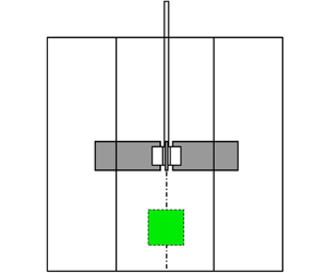
We use 2D2C PIV in the vertical $(x,z)$ plane indicated in figure 5. This figure also shows the field of view which is aligned with that vertical plane and has its centre offset by only $3\pm 1\ {\rm mm}$ in the $y$ direction from the centreline.

Figure 5. Measurement plane location.

The PIV set-up is composed of a camera, a laser, a set of lenses and mirrors to shape the laser beam into a thin light sheet and a Lavision PTU synchronisation unit and a recording computer with Davis 10 from Lavision.

4.2.1. Camera

The camera used is a Phantom v2640 with full sensor image ($2048\ {\rm px} \times 1952\ {\rm px}$). A Nikon macro Nikkor 200 mm lens is used with f#8. The extremity of the lens is at 93 mm from the glass. The field of view size is $C_{1}\times C_{2} \approx 27\ {\rm mm} \times 28\ {\rm mm}$ (see figure 5) with a magnification factor of $14.1\ \mathrm {\mu } {\rm m}\ {\rm px}^{-1}$.

The acquisition is done by packets of five time-resolved images. The packet acquisition frequency is 6 Hz to ensure decorrelation between successive packets. The acquisition frequency for the five images within each packet varies from 1.25 to 3 kHz depending on type of blade and rotor speed. This parameter is specifically set for each configuration to ensure a turbulent fluctuation displacement between two frames of around 5 px (corresponding to about 1 standard deviation) and maximum 10 px (observed with samples during the experiments).

4.2.2. Laser, mirrors and lenses

The laser used is a Blizz 30W high speed frequency laser from InnoLas. The laser is optimised at 40 kHz with $750\ \mathrm {\mu } {\rm J}\ {\rm pulse}^{-1}$ at $532\ {\rm nm}$ wavelength and $M^2 < 1.3$. For the experiments it was set to around $500\ \mathrm {\mu } {\rm J}\ {\rm pulse}^{-1}$ because of the smaller frequency used. The laser frequency is set according to the camera time-resolved recording frequency. The focal lengths of the spherical and the cylindrical lenses are $+$800 mm and $-$80 mm, respectively (beam waist set in the centre of the field of view). The laser sheet height obtained is around 60 mm and its width is 0.6 mm at the waist (which is close to the centreline of the mixer) with a Rayleigh length of 400 mm. Therefore, the laser sheet's width is constant over the field of view.

4.2.3. Seeding

Mono-disperse polystyrene Spherotech particles of diameter $5.33\ \mathrm {\mu }{\rm m}$ are used. They maximise the concentration in the flow and lead to enough particles within each interrogation window. The background noise is around 30 counts. There are on average about 10 particles per interrogation window of $32\ {\rm px} \times 32\ {\rm px}$ if a threshold of 50 counts is used to select most particles. This is consistent with the criteria of Keane & Adrian (Reference Keane and Adrian1991). Among these particles, there is on average 6.5 particles higher than 100 counts per interrogation window.

4.2.4. Processing

The calibration is done with LaVision 058-5 plate. The PIV processing is done with the Matpiv toolbox modified at LMFL. It is a classical multigrid and multipass cross-correlation algorithm (Willert & Gharib Reference Willert and Gharib1991; Soria Reference Soria1996). Here four passes are used, starting with $64\ {\rm px} \times 64\ {\rm px}$, then $48\ {\rm px} \times 48\ {\rm px}$ and finishing with two $32\ {\rm px} \times 32\ {\rm px}$ passes. Before the final pass, image deformation is used to improve the results (Scarano Reference Scarano2001; Lecordier & Trinité Reference Lecordier and Trinité2004). An overlap between interrogation windows of 62 % is used, leading to vector spacing of about 0.17 mm. The final grid has then 159 points in the horizontal direction and 167 in the vertical one.

4.3. Description of the experimental measurements

4.3.1. The PIV resolution

The PIV resolution of the experiment (i.e. interrogation window size) is presented in table 1. In terms of the Kolmogorov length $\eta \equiv (\nu ^{3}/\langle \overline {\epsilon ^{\prime }}\rangle )^{1/4}$, where the angular brackets signify a space average over the PIV field of view, the resolution is between $3.4\eta$ and $5.1\eta$ depending on configuration. For those configurations where the interrogation window size is higher than $3\eta$ the turbulence dissipation rate might be underestimated when denoised properly (Foucaut et al. Reference Foucaut, George, Stanislas and Cuvier2021). However, this underestimation remains acceptable for interrogation window size smaller than $5\eta$ where less than 30 % of uncertainty (filtering effect) is expected according to Laizet, Nedić & Vassilicos (Reference Laizet, Nedić and Vassilicos2015) and Lavoie et al. (Reference Lavoie, Avallone, De Gregorio, Romano and Antonia2007).

Table 1. The PIV resolution.

4.3.2. Statistical convergence

For each configuration, 150 000 velocity fields are recorded in time including 50 000 fully uncorrelated velocity field samples for convergence. Averaging over time is not sufficient for convergence and we therefore also apply averaging over space which greatly improves the convergence. It corresponds to $150\,000 \times 164 \times 78 \approx 1.9\times 10^9$ points for one-point statistics, where $164 \times 78$ is the number of points associated with the vector spacing. For two-point statistics, some spatial points are not available depending on the separation vector size and direction. For zero separation vector, $150\,000 \times 164 \times 78 \approx 1.9 \times 10^9$ points are available for convergence, but for the largest separation vector in the $r_x$ direction there are only $150\,000 \times 164 \approx 2.4 \times 10^7$ points available and in the $r_z$ direction only $150\,000 \times 78 \approx 1.2 \times 10^7$ are available.

The most important results in this paper are reported with error bars quantifying convergence and computed with a bootstrapping method. The central limit theorem is applied to averages over subgroups of samples of the quantity of interest. For each quantity, 600 subgroups containing 83 time steps with at least $159$ spatial points are used for the computation of an error bar. This method is robust and provides accurate estimations without having to define the number of independent points. The resulting error bars are also representative of the convergence of third-order two-point statistics plotted here without error bars as the number of points used is the same.

4.3.3. Peak locking

When a particle is too small, its correlation peak position fitting results are biased towards integer values. Therefore, the displacement between two images is more likely to be an integer number of pixels. This peak-locking error (as it is called; Raffel et al. Reference Raffel, Willert, Scarano, Kähler, Wereley and Kompenhans2018) is systematic (bias error) and is therefore visible on the velocity probability distribution functions (sine modulation) but does not usually impact mean quantities of turbulent flow if enough dynamic is used (here high dynamic is selected of about 5 px for one standard deviation; see Christensen (Reference Christensen2004)). Peak locking can be reduced by increasing particle diffraction spot using camera lens aperture f# number. However, an increased f# number reduces the brightness of the particles and therefore the number of visible particles. In this experiment, f#8 is used as a compromise and some peak locking is still visible. The impact on the results is analysed in § 3 of the supplementary material available at https://doi.org/10.1017/jfm.2024.220 where we show that energy spectra and averages of two-point velocity quantities such as the interscale turbulent energy transfer rate are unaffected by peak locking.

4.3.4. Defining parameters

The defining parameters of the experiment are presented in table 2. The rotation frequency $F$ is either 1 or 1.5 Hz. The global Reynolds number is $Re={2{\rm \pi} F R^2}/{\nu }$, where $R=D/2\approx 11.25\ {\rm cm}$ is an estimate of the rotor radius. The value of $Re$ is large, higher than $8 \times 10^4$, and the flow is therefore turbulent.

Table 2. Main parameters of the experiment: vel r.m.s. (${\rm m} \ {\rm s}^{-1}$) stands for $\sqrt {\overline {\langle u_x^{\prime 2}\rangle } + \overline {\langle u_z^{\prime 2}\rangle }}$.

The Rossby number is estimated as $Ro={U}/{2 \varOmega R}$, where $U$ (following Baroud et al. Reference Baroud, Plapp, She and Swinney2002) is the maximum fluctuating velocity in all our samples, $R$ is as an estimate of the integral length scale of the turbulence and $\varOmega =2{\rm \pi} F$. Our values of $Ro$ range between $10^{-1}$ and $1$ and are therefore intermediate between those of fast-rotating and non-rotating turbulence. However, the rotor rotation speed $\varOmega$ is not representative of flow rotation because the baffles break the flow rotation as explained in Nagata (Reference Nagata1975). Therefore, the Rossby number is probably severely underestimated and the rotation is not expected to affect significantly the turbulence behaviour in our experiment.

4.3.5. Basic turbulent flow properties

The main turbulent parameters are presented in table 3. They include the turbulence dissipation rate $\langle \overline {\epsilon ^{\prime }}\rangle$ averaged over time (overbar) and over space in our field of view (angle brackets), the resulting Kolmogorov length scale $\eta$ (computed with $\langle \overline {\epsilon ^{\prime }}\rangle$) and the Taylor length $\lambda$. These parameters are provided as reference and are used in the paper to non-dimensionalise results.

Table 3. Main turbulence parameters. The Kolmogorov length scale is calculated as $\eta \equiv (\nu ^{3}/\langle \overline {\epsilon ^{\prime }}\rangle )^{1/4}$. The Taylor length and the Reynolds number $Re_{\lambda }$ are calculated as in § 1.2 of the supplementary material.

The Taylor-length-based Reynolds number $Re_{\lambda }$ (see discussion on its estimation in § 1.2 of the supplementary material) is higher than 480 in all four configurations. All the four flows that we study are therefore highly turbulent.

In figure 6(b) we plot the mean flow velocity for one of our four configurations but the plot is representative of all four configurations. The mean flow velocity is oriented vertically from bottom to top and is not negligible in magnitude. Within our field of view, it is horizontally uniform and accelerates by about 7 % from bottom to top. These observations are consistent with the overall mean flow structure identified by Nagata (Reference Nagata1975) and shown in figure 6(a).

Figure 6. (a) Schematic of mean flow in a mixer with baffles (Nagata Reference Nagata1975). (b) Mean flow measurement within the measurement plane shown as a green square in (a).

4.3.6. Two-dimensional two-component truncations and estimates of three-dimensional three-component statistics

The various terms in the equations of the previous sections require three-component velocity fields in three-dimensional space to be calculated. However, our measurements are performed with 2D2C PIV. We can therefore only calculate 2D2C truncations of three-dimensional three-component (3D3C) statistics and in a few cases (§§ 5 and 6) we estimate 2D2C surrogates of 3D3C terms.

5. Two-point turbulence production rates

We start our data analysis with an assessment of two-point turbulence production rates. We define our coordinate system such that components $i=1$, $i=2$ and $i=3$ correspond to the $x$, $y$ and $z$ directions, respectively, and therefore $(r_1 , r_2 , r_3 )= (r_x , r_y, r_z )$ and $(X_1 , X_2 , X_3 )= (X_x , X_y , X_z )$. The sums defining $P_r=-\overline {\delta u_j ^\prime \delta u_i ^\prime }({\partial \delta \overline {u_i}}/{\partial r_j})$, $P_{Xr}^s=-\overline {u_{Xj} ^\prime \delta u_i ^\prime }({\partial \delta \overline {u_i}}/{\partial X_j})$, $P_X=-\overline {u_{Xj} ^\prime u_{Xi} ^\prime }({\partial \overline {u_{Xi}}}/{\partial X_j})$ and $P_{Xr}^l=-\overline { \delta u_j ^\prime u_{Xi} ^\prime }({\partial \delta \overline {u_i}}/{\partial X_j})$ are sums of nine terms of which our 2D2C PIV has access to four. Our data therefore allow only truncations to be calculated directly and we start with the truncation of $P_r$:

(5.1)\begin{equation} \widetilde{P_r}={-}\overline{\delta u_{x}^{\prime} \delta u_{x}^{\prime}} \frac{\partial \overline{\delta u_{x}}}{\partial r_x} - \overline{\delta u_{x}^{\prime} \delta u_{z}^{\prime}} \frac{\partial \overline{\delta u_{z}}}{\partial r_x} - \overline{\delta u_{z}^{\prime} \delta u_{x}^{\prime}} \frac{\partial \overline{\delta u_{x}}}{\partial r_z} - \overline{\delta u_{z}^{\prime} \delta u_{z}^{\prime}} \frac{\partial \overline{\delta u_{z}}}{\partial r_z} \end{equation}

with

(5.2)\begin{equation} \overline{\delta u_{y}^{\prime} \delta u_{y}^{\prime}} \frac{\partial \overline{\delta u_{y}}}{\partial r_y} + \overline{\delta u_{x}^{\prime} \delta u_{y}^{\prime}} \frac{\partial \overline{\delta u_{y}}}{\partial r_x} + \overline{\delta u_{x}^{\prime} \delta u_{y}^{\prime}} \frac{\partial \overline{\delta u_{x}}}{\partial r_y} + \overline{\delta u_{z}^{\prime} \delta u_{y}^{\prime}} \frac{\partial \overline{\delta u_{y}}}{\partial r_z} + \overline{\delta u_{z}^{\prime} \delta u_{y}^{\prime}} \frac{\partial \overline{\delta u_{z}}}{\partial r_y} \end{equation}

being the difference between $\widetilde {P_r}$ and $P_r$. We know from our measurements and from Nagata (Reference Nagata1975) that the mean flow is vertical in our field of view which is small and very close to the centreline of the tank. Hence, we can readily neglect all the terms making the difference between $\widetilde {P_r}$ and $P_r$ except $\overline {\delta u_{z}^{\prime } \delta u_{y}^{\prime }} ({\partial \overline {\delta u_{z}}}/{\partial r_y})$. Making the assumption that $\overline {\delta u_{z}^{\prime } \delta u_{y}^{\prime }} ({\partial \overline {\delta u_{z}}}/{\partial r_y}) \approx \overline {\delta u_{z}^{\prime } \delta u_{x}^{\prime }} ({\partial \overline {\delta u_{z}}}/{\partial r_x})$ we form the following surrogate estimate of $P_r$:

(5.3)\begin{equation} \widetilde{\widetilde{P_r}}={-}\overline{\delta u_{x}^{\prime} \delta u_{x}^{\prime}} \frac{\partial \overline{\delta u_{x}}}{\partial r_x} - 2\overline{\delta u_{x}^{\prime} \delta u_{z}^{\prime}} \frac{\partial \overline{\delta u_{z}}}{\partial r_x} - \overline{\delta u_{z}^{\prime} \delta u_{x}^{\prime}} \frac{\partial \overline{\delta u_{x}}}{\partial r_z} - \overline{\delta u_{z}^{\prime} \delta u_{z}^{\prime}} \frac{\partial \overline{\delta u_{z}}}{\partial r_z}. \end{equation}

Similarly, we have the following truncations and surrogate estimates for the other three two-point turbulence production rates:

(5.4)\begin{equation} \widetilde{P_{Xr}^s}={-}\overline{u_{Xx}^{\prime} \delta u_{x}^{\prime}} \frac{\partial \overline{\delta u_{x}}}{\partial X_x} - \overline{u_{Xx}^{\prime} \delta u_{z}^{\prime}} \frac{\partial \overline{\delta u_{z}}}{\partial X_x} - \overline{u_{Xz}^{\prime} \delta u_{x}^{\prime}} \frac{\partial \overline{\delta u_{x}}}{\partial X_z} - \overline{u_{Xz}^{\prime} \delta u_{z}^{\prime}} \frac{\partial \overline{\delta u_{z}}}{\partial X_z} \end{equation}

and

(5.5)\begin{gather} \widetilde{\widetilde{P_{Xr}^s}}={-}\overline{u_{Xx}^{\prime} \delta u_{x}^{\prime}} \frac{\partial \overline{\delta u_{x}}}{\partial X_x} - 2\overline{u_{Xx}^{\prime} \delta u_{z}^{\prime}} \frac{\partial \overline{\delta u_{z}}}{\partial X_x} - \overline{u_{Xz}^{\prime} \delta u_{x}^{\prime}} \frac{\partial \overline{\delta u_{x}}}{\partial X_z} - \overline{u_{Xz}^{\prime} \delta u_{z}^{\prime}} \frac{\partial \overline{\delta u_{z}}}{\partial X_z}; \end{gather}

(5.6)\begin{gather}\widetilde{P_X}={-}\overline{u_{Xx}^{\prime} u_{Xx}^{\prime}} \frac{\partial \overline{u_{Xx}}}{\partial X_x} - \overline{u_{Xx}^{\prime} u_{Xz}^{\prime}} \frac{\partial \overline{u_{Xz}}}{\partial X_x} - \overline{u_{Xz}^{\prime} u_{Xx}^{\prime}} \frac{\partial \overline{u_{Xx}}}{\partial X_z} - \overline{u_{Xz}^{\prime} u_{Xz}^{\prime}} \frac{\partial \overline{u_{Xz}}}{\partial X_z} \end{gather}

and

(5.7)\begin{gather} \widetilde{\widetilde{P_X}}={-}\overline{u_{Xx}^{\prime} u_{Xx}^{\prime}} \frac{\partial \overline{u_{Xx}}}{\partial X_x} - 2\overline{u_{Xx}^{\prime} u_{Xz}^{\prime}} \frac{\partial \overline{u_{Xz}}}{\partial X_x} - \overline{u_{Xz}^{\prime} u_{Xx}^{\prime}} \frac{\partial \overline{u_{Xx}}}{\partial X_z} - \overline{u_{Xz}^{\prime} u_{Xz}^{\prime}} \frac{\partial \overline{u_{Xz}}}{\partial X_z}; \end{gather}

(5.8)\begin{gather}\widetilde{P_{Xr}^l}={-}\overline{\delta u_{x}^{\prime} u_{Xx}^{\prime}} \frac{\partial \overline{\delta u_{x}}}{\partial X_x} - \overline{\delta u_{x}^{\prime} u_{Xz}^{\prime}} \frac{\partial \overline{\delta u_{z}}}{\partial X_x} - \overline{\delta u_{z}^{\prime} u_{Xx}^{\prime}} \frac{\partial \overline{\delta u_{x}}}{\partial X_z} - \overline{\delta u_{z}^{\prime} u_{Xz}^{\prime}} \frac{\partial \overline{\delta u_{z}}}{\partial X_z} \end{gather}

and

(5.9)\begin{equation} \widetilde{\widetilde{P_{Xr}^l}}={-}\overline{\delta u_{x}^{\prime} u_{Xx}^{\prime}} \frac{\partial \overline{\delta u_{x}}}{\partial X_x} - 2\overline{\delta u_{x}^{\prime} u_{Xz}^{\prime}} \frac{\partial \overline{\delta u_{z}}}{\partial X_x} - \overline{\delta u_{z}^{\prime} u_{Xx}^{\prime}} \frac{\partial \overline{\delta u_{x}}}{\partial X_z} - \overline{\delta u_{z}^{\prime} u_{Xz}^{\prime}} \frac{\partial \overline{\delta u_{z}}}{\partial X_z}. \end{equation}

The results are presented in § 2 of the supplementary material and our data support the hypothesis already expressed at the end of the fourth paragraph of § 3 that, for the turbulent flows considered here and for scales small enough compared to the large scales of the flow, two-point production $P^{s}_{Xr}$ may be neglected in the small-scale energy equation (2.4). However, $P_r$, while smaller than all other terms, may not be convincingly negligible in that equation. In the intermediate layer of fully developed turbulent channel flow, $P_r$ was also found by Apostolidis et al. (Reference Apostolidis, Laval and Vassilicos2023) not to be negligible at scales comparable to and larger than the Taylor length, but the ratio of $P_r$ to turbulence dissipation rate was significantly higher than in the present flow. The supplementary material also includes results for $P_X$ and $P^{l}_{Xr}$ in its § 2, suggesting that $P^{l}_{Xr}$ may but $P_X$ may not be negligible in the large-scale energy equation (2.8).

6. Small-scale linear transport terms

In the theory used in the present paper, we neglect two-point production in the small-scale energy equation (2.4) but not in the large-scale energy equation (2.8). We return to this approximation at the start of § 8.4. We now focus on (2.4) and ask whether we can justify simplifying it further by neglecting the linear transport rate $( \overline {\boldsymbol {u_X}}\boldsymbol {\cdot }\boldsymbol {\nabla _X} +\boldsymbol {\delta \bar {u}}\boldsymbol {\cdot }\boldsymbol {\nabla _r} )\frac {1}{2} \overline {|\boldsymbol {\delta u^\prime }|^2}$. The results are presented in § 2 of the supplementary material where we find grounds to neglect some but not all of the terms in $( \overline {\boldsymbol {u_X}}\boldsymbol {\cdot }\boldsymbol {\nabla _X} +\boldsymbol {\delta \bar {u}}\boldsymbol {\cdot }\boldsymbol {\nabla _r})\frac {1}{2} \overline {|\boldsymbol {\delta u^\prime }|^2}$ from the small-scale energy equation (2.4) at small enough scales. Note, however, that the conclusions of the following two sections can be obtained (see Chen & Vassilicos Reference Chen and Vassilicos2022) both with and without this term in (2.4) (with the only potential exception of the last sentence of § 8.4 which may need to be qualified). For ease of presentation we therefore consider the following simplified form of this equation for the turbulent flow region studied here:

(6.1)\begin{align} &\boldsymbol{\nabla_X}\boldsymbol{\cdot}(\overline{\boldsymbol{u_X}^\prime |\boldsymbol{\delta u}^\prime|^2}) + \boldsymbol{\nabla_r}\boldsymbol{\cdot}(\overline{\boldsymbol{\delta u}^\prime |\boldsymbol{\delta u}^\prime|^2}) + 2\boldsymbol{\nabla_X}\boldsymbol{\cdot}\overline{(\boldsymbol{\delta u ^\prime}\delta p ^\prime)} \nonumber\\ &\quad \approx \frac{\nu}{2} (\boldsymbol{\nabla_X} ^2+ \boldsymbol{\nabla_r} ^2) \overline{|\boldsymbol{\delta u^\prime}|^2} - \frac{1}{2} \left( \overline{\epsilon^{\prime +}} + \overline{\epsilon^{\prime -}} \right) , \end{align}

where $\overline {\epsilon ^{\prime +}}$ and $\overline {\epsilon ^{\prime -}}$ are $\overline {\epsilon ^{\prime }}$ at $\boldsymbol {\zeta }^+$ and $\boldsymbol {\zeta }^-$, respectively.

It is worth pointing out that a careful look at the results in § 2 of the supplementary material suggests that the approximation (6.1) does not necessarily hold for large enough values of $r_x$ and/or $r_z$. Apostolidis et al. (Reference Apostolidis, Laval and Vassilicos2023) found, in a very different non-homogeneous turbulent flow (namely the intermediate region of fully developed turbulent channel flow), that (6.1) is not a representative approximation at scales comparable with and larger than $\lambda$ whereas we do assume it to be a good approximation at such scales (if they are not too large) in the flow region of the non-homogeneous turbulent flows considered here.

7. Second-order structure functions

We now adopt the approach of Chen & Vassilicos (Reference Chen and Vassilicos2022) which is based on inner and outer similarity. In effect, we assume that regions of space exist in the flow where the nonlinear and non-local dynamics of the small-scale turbulence are similar at different places within the region. We therefore start with a hypothesis of inner and outer similarity for the second-order structure function $\overline {|\boldsymbol {\delta u^\prime }|^2}$, namely

(7.1)\begin{equation} \overline{|\boldsymbol{\delta u}^\prime|^2}=V_{O2}^2(\boldsymbol{X})f_{O2} \left( \frac{\boldsymbol{r}}{l_O}\right) \end{equation}

for $\vert \boldsymbol {r}\vert \gg l_I$ and

(7.2)\begin{equation} \overline{|\boldsymbol{\delta u}^\prime|^2}=V_{I2}^2(\boldsymbol{X})f_{I2} \left( \frac{\boldsymbol{r}}{l_I}\right) \end{equation}

for $\vert \boldsymbol {r}\vert \ll l_O$, where the inner length scale $l_I$ depends on viscosity and is much smaller than the outer length scale $l_O$ which does not depend on viscosity, i.e. $l_{I}= l_{I}(\boldsymbol {X}) \ll l_{O} = l_{O}(\boldsymbol {X})$ for large enough Reynolds number. The outer length scale can be thought of as an integral length of the order of the blade size $R=D/2$ and is assumed to be smaller than the extent of the similarity region where (7.1) and (7.2) hold. Statistical homogeneity is a special case of our inner and outer similarity hypotheses where $V_{O2}$, $V_{I2}$, $l_O$ and $l_I$ are independent of $\boldsymbol {X}$. In the following section we apply the approach of Chen & Vassilicos (Reference Chen and Vassilicos2022) to the small-scale energy balance (6.1).

It is natural to expect the outer characteristic velocity $V_{O2}$ to be independent of viscosity but the inner characteristic velocity $V_{I2}$ to depend on it. The ratios $V_{I2}/V_{O2}$ and $l_{I}/l_{O}$ must therefore be functions of a local Reynolds number $Re_{O} = V_{O2} l_{O}/\nu$ and we write $V_{I2}/V_{O2} = g_{2} (Re_{O}, \boldsymbol {X})$, $l_{I}/l_{O}=g_{l}(Re_{O}, \boldsymbol {X})$, these two functions having to tend to zero as $Re_O$ tends to infinity. This is the only assumption we make about these two ratios $V_{I2}/V_{O2}$ and $l_{I}/l_{O}$. In § 8.2 we obtain their $Re_O$ dependence from the small-scale turbulent energy budget, i.e. from the Navier–Stokes equation.

The inner and outer similarity forms overlap in the range $l_{I}\ll \vert \boldsymbol {r}\vert \ll l_O$, hence

(7.3)\begin{equation} f_{O2} \left( \frac{\boldsymbol{r}}{l_O}\right) = g_{2}^{2} (Re_{O}, \boldsymbol{X}) f_{I2} \left( \frac{\boldsymbol{r}}{l_O}g_{l}^{{-}1}\right) \end{equation}

in this intermediate range. Given that the left-hand side of this equation does not depend on $Re_O$, the derivative with respect to $Re_O$ of the right-hand side cancels and we obtain

(7.4)\begin{equation} g_{l} \frac{{\rm d}g_{2}^{2}}{{\rm d}Re_O} f_{I2}(\boldsymbol{\rho}) = g_{2}^{2} \frac{{\rm d}g_{l}}{{\rm d}Re_O} \rho_{j}\frac{\partial}{\partial \rho_{j}} f_{I2} (\boldsymbol{\rho}), \end{equation}

where there is an implicit sum over $j=1,2,3$ and $\boldsymbol {\rho }=(\rho _{1}, \rho _{2}, \rho _{3})= \boldsymbol {r}/l_{I}$. It follows that $\rho _{j}({\partial }/{\partial \rho _{j}}) f_{I2} (\boldsymbol {\rho })$ is proportional to $f_{I2}(\boldsymbol {\rho })$. To solve for $f_{I2}$ we adopt spherical coordinates $(\rho, \theta, \phi )$ for $\boldsymbol {\rho }$, where $\theta$ varies from $0$ to ${\rm \pi}$ and vanishes if $\boldsymbol {\rho }$ is aligned with the $y$ axis and where $\phi$ varies from $0$ to $2{\rm \pi}$ and is equal to $0$ or ${\rm \pi} /2$ if $\boldsymbol {\rho }$ is aligned with the $x$ or the $z$ axis, respectively. The proportionality between $\rho _{j}({\partial }/{\partial \rho _{j}} )f_{I2} (\boldsymbol {\rho })$ and $f_{I2}(\boldsymbol {\rho })$ becomes $n f_{I2}(\rho, \theta, \phi ) = \rho ({\partial }/{\partial \rho }) f_{I2}(\rho, \theta, \phi )$ in terms of a dimensionless proportionality constant $n$ and the solution to this equation is

(7.5)\begin{equation} f_{I2} = \rho^{n} F(\theta, \phi), \end{equation}

where $F$ is an unknown function of angles $\theta$ and $\phi$. Note that (7.5) holds in the intermediate range $l_{I}\ll \vert \boldsymbol {r}\vert \ll l_O$. Returning to (7.3), we get

(7.6)\begin{equation} g_{2}^{2}(Re_{O},\boldsymbol{X})g_{l}^{{-}n}(Re_{O},\boldsymbol{X}) = A_1 ,\end{equation}

where the dimensionless coefficient $A_1$ is independent of $Re_{O}$ and $\boldsymbol {X}$.

At this stage we follow Chen & Vassilicos (Reference Chen and Vassilicos2022) and use their hypothesis of inner–outer equivalence for dissipation according to which there is an inner and an outer way to estimate the turbulence dissipation rate: $\overline {\epsilon ^{\prime }} \sim V_{O2}^{3}/l_{O} \sim V_{I2}^{3}/l_{I}$, where the proportionality coefficients are independent of $Re_{O}$ but can depend on $\boldsymbol {X}$. We actually derive this hypothesis in § 8.3 and our derivation shows clearly that it has nothing to do with Kolmogorov's scale-by-scale equilibrium. At this stage, it provides the additional constraint $g_{2}^{3}(Re_{O}) g_{l}^{-1}(Re_{O}) = A_2$, where the coefficient $A_2$ is independent of $Re_O$. Combined with this additional constraint, (7.6) yields $n=2/3$ (and $A_3=A^{3/2}$, which means that $A_2$ is also independent of $\boldsymbol {X}$) and therefore

(7.7)\begin{equation} \overline{|\boldsymbol{\delta u}^\prime|^2}=C (\overline{\epsilon^{\prime}} r)^{2/3} F(\theta, \phi) \end{equation}

in the intermediate range $l_{I}\ll r=\vert \boldsymbol {r}\vert \ll l_O$. Note that, reflecting the dimensionless coefficients in $\overline {\epsilon ^{\prime }} \sim V_{O2}^{3}/l_{O} \sim V_{I2}^{3}/l_{I}$, the dimensional coefficient $C$ can vary in space but is independent of Reynolds number. The dependence of these dimensional coefficients, and $C$ in particular, on spatial position is an obvious difference from Kolmogorov's prediction for the second-order structure function which is limited to locally homogeneous turbulence. This difference highlights the underlying difference in the way that our result (7.7) was obtained compared with Kolmogorov's derivation of his corresponding prediction which resembles (7.7) in the scaling $(\overline {\epsilon ^{\prime }} r)^{2/3}$ but is otherwise different (see Frisch (Reference Frisch1995), Pope (Reference Pope2000) and § 2 of Chen & Vassilicos (Reference Chen and Vassilicos2022)).

We can refine our hypothesis of similarity by replacing it with a hypothesis of isotropic similarity which is a hypothesis of similarity for each component of $\boldsymbol {\delta u^\prime }$, namely

(7.8)\begin{equation} \overline{(\delta u_{j}^\prime)^2}=V_{O2}^2(\boldsymbol{X})f_{O2, j} \left( \frac{\boldsymbol{r}}{l_O}\right) \end{equation}

for $\vert \boldsymbol {r}\vert \gg l_I$ and

(7.9)\begin{equation} \overline{(\delta u_{j}^\prime)^2}=V_{I2}^2(\boldsymbol{X})f_{I2, j} \left( \frac{\boldsymbol{r}}{l_I}\right) \end{equation}

for $\vert \boldsymbol {r}\vert \ll l_O$ for every $j=1,2,3$. This is not an assumption of isotropy because neither the functions $f_{O2, j}$ nor the functions $f_{I2,j}$ are necessarily the same for different $j=1,2,3$. The argument leading to (7.7) can be repeated for every $j=1,2,3$ yielding

(7.10)\begin{equation} \overline{(\delta u_{j}^\prime)^2}=C_{j} (\overline{\epsilon^{\prime}} r)^{2/3} F_{j}(\theta, \phi) \end{equation}

in the intermediate range $l_{I}\ll r=\vert \boldsymbol {r}\vert \ll l_O$. The dimensionless coefficient $C_j$ may vary with $j$ and with $\boldsymbol {X}$ and the dimensionless function $F_j$, which is independent of $\boldsymbol {X}$ and of $r\equiv \vert \boldsymbol {r}\vert$, may also vary with $j$. The determination of the inner length scale $l_I$ requires the small-scale energy balance (6.1). This is done in § 8. We complete the present section by confronting prediction (7.10) with our PIV data. This prediction is similar to Kolmogorov's prediction for second-order structure functions but it was derived without the homogeneity assumption required by Kolmogorov's theory and without Kolmogorov's scale-by-scale equilibrium which forms the physical basis of Kolmogorov's dimensional analysis.

7.1. Second-order structure function measurements

We compute the normalised structure functions $\langle \overline {(\delta u_{j}^\prime )^2}/ \overline {\epsilon ^{\prime }}^{2/3} \rangle$ for $j=1$ (velocity fluctuations along the $x$ axis) and $j=3$ (velocity fluctuations along the $z$ axis) by averaging over time, i.e. over our 150 000 samples (which correspond to 50 000 uncorrelated samples), and also averaging over $\boldsymbol {X}$, i.e. over the planar space of our field of view. The additional averaging over space is necessary for convergence of our statistics (see in § 4 in the supplementary material). The normalised structure functions $\overline {(\delta u_{j}^\prime )^2}/\overline {\epsilon ^{\prime }}^{2/3}$ are therefore calculated by averaging over available points in the field of view in 150 000 velocity field samples in this field of view. For two-point statistics, there are between $1.2 \times 10^7$ and $1.9 \times 10^9$ points available for convergence, depending on two-point separation vector, using both space and time averaging as explained in § 4.3.2.

Given that (7.10) implies $\langle \overline {(\delta u_{j}^\prime )^2}/\overline {\epsilon ^{\prime }}^{2/3}\rangle = \langle C_{j}\rangle r^{2/3} F_{j}(\theta, \phi )$, we plot in figure 7 the compensated structure functions $\langle \overline {(\delta u_{x}^\prime )^2}/\overline {\epsilon ^{\prime }}^{2/3} \rangle r^{-2/3}$ ( $j=1$) versus $r_{x}/D$ (figure 7a) and versus $r_{z}/D$ (figure 7b) and $\langle \overline {(\delta u_{z}^\prime )^2}/\overline {\epsilon ^{\prime }}^{2/3} \rangle r^{-2/3}$ ( $j=3$) versus $r_{x}/D$ (figure 7c) and versus $r_{z}/D$ (figure 7d). This is the intermediate-range data collapse suggested by (7.10) for all four configurations considered here. The dependence on $r_x$ represents the dependence on $r$ for $\theta = {\rm \pi}/2$ and $\phi =0$ whereas the dependence on $r_z$ represents the dependence on $r$ for $\theta = {\rm \pi}/2$ and $\phi ={\rm \pi} /2$. The average turbulence dissipation rate $\langle \overline {\epsilon ^{\prime }}\rangle$ varying by a factor larger than 4 across our four different configurations (see table 3), figure 7 suggests that the collapse of the compensated structure functions in figure 7 is satisfactory. The exponent of the power-law dependence of these structure functions on $r_x$ and $r_z$ (in an expected intermediate range of scales much smaller than $R=D/2$) appears close to but not exactly $2/3$ and seems to vary a little around $2/3$ from plot to plot in figure 7. The theory presented above and yielding (7.7) and (7.10) may be a leading-order theory with different higher-order corrections for different $j$ components. Such corrections are beyond the scope of the present paper, but noting from the plots in figure 7 that there may be opposite corrections to the $2/3$ scaling, we now consider the $r_x$ and $r_z$ dependencies of the normalised structure function $\langle \overline {(\delta u_x^{\prime 2} + \delta u_z^{\prime 2})} /\overline {\epsilon ^{\prime }}^{2/3} \rangle$. Equation (7.10) implies

(7.11)\begin{equation} \langle \overline{(\delta u_x^{\prime 2} + \delta u_z^{\prime 2})}/\overline{\epsilon^{\prime}}^{2/3} \rangle =r^{2/3} [\langle C_{1} \rangle F_{1}(\theta, \phi) +\langle C_{3}\rangle F_{3}(\theta, \phi)] . \end{equation}

Figure 7. Compensated structure functions. (a) Compensated $\overline {\delta u_x ^{\prime 2}}$ in $r_x$ direction. (b) Compensated $\overline {\delta u_x ^{\prime 2}}$ in $r_z$ direction. (c) Compensated $\overline {\delta u_z ^{\prime 2}}$ in $r_x$ direction. (d) Compensated $\overline {\delta u_z ^{\prime 2}}$ in $r_z$ direction.

This compensated normalised structure function is presented in figure 8 as a function of $r_{x}/D$ (i.e. $r/D$ for $\theta = {\rm \pi}/2$ and $\phi =0$) in one plot and of $r_{z}/D$ (i.e. $r/D$ for $\theta = {\rm \pi}/2$ and $\phi ={\rm \pi} /2$) in the other. Once again, the resulting collapse of the structure functions for the four different configurations is acceptable given the wide variation of $\langle \overline {\epsilon ^{\prime }}\rangle$ from one configuration to the other. To look at the power-law scaling more finely, we estimate the logarithmic slopes of $S\equiv \langle \overline {(\delta u_x^{\prime 2} + \delta u_z^{\prime 2})}/\overline {\epsilon ^{\prime }}^{2/3} \rangle$ versus both $r_x$ and $r_z$, i.e. ${{\rm d} \log S}/{{\rm d} \log r_x}$ and ${{\rm d} \log S}/{{\rm d} \log r_z}$, which we plot versus $r_x$ and $r_z$, respectively, in figures 9(a) and 9(b). A well-defined plateau appears in both directions for $r_{x}, r_{z}\ll R=D/2$ which confirms the power-law behaviour of $S$. The value of the plateau is the power-law exponent and it is slightly different in the two directions: it lies between $2/3 \approx 0.66$ and $0.7$ in the $r_x$ direction, which is very close to the theory's prediction, but between $0.5$ and $0.6$ in the $r_z$ direction, which is further away from it.

Figure 8. Compensated structure function $\overline {(\delta u_x^{\prime 2} + \delta u_z^{\prime 2})}$. (a) The $r_x$ direction. (b) The $r_z$ direction.

Figure 9. Logarithmic slope of $S\equiv \langle \overline {(\delta u_x^{\prime 2} + \delta u_z^{\prime 2})}/\overline {\epsilon ^{\prime }}^{2/3} \rangle$. (a) The $r_x$ direction. (b) The $r_z$ direction.

We must leave it for future study to determine whether the deviation from $n=2/3$ that we observe in the vertical $r_z$ direction is a finite-Reynolds-number effect or whether it results from deviations from outer and/or inner isotropic similarity of second-order structure functions. The good agreement with $n=2/3$ in the $r_x$ direction is nevertheless encouraging and so, in the following section, we use $n=2/3$ in conjunction with an analysis of the small-scale energy budget to predict the relations between $l_I$ and $l_O$ and between $V_{I2}$ and $V_{O2}$. Perhaps more importantly, though, this analysis also leads to predictions concerning nonlinear interscale and interspace turbulent energy transfer rates which do not critically depend on the value of the exponent $n$ and which we also subject to experimental checks.

8. Small-scale turbulent energy budgets

Following Chen & Vassilicos (Reference Chen and Vassilicos2022) who assume that regions exist in the flow where the nonlinear and non-local dynamics of the small scale turbulence are similar at different places within the region, we now introduce, for such a region, inner and outer similarity form for every term on the left-hand side of (6.1).

Outer similarity for $\vert \boldsymbol {r}\vert \gg l_I$:

(8.1)\begin{gather} \boldsymbol{\nabla_X}\boldsymbol{\cdot}(\overline{\boldsymbol{u_X}^\prime |\boldsymbol{\delta u}^\prime|^2}) = \frac{V_{OX}^3(\boldsymbol{X})}{l_{O}}f_{OX} \left( \frac{\boldsymbol{r}}{l_{O}}\right), \end{gather}

(8.2)\begin{gather}\boldsymbol{\nabla_r}\boldsymbol{\cdot}(\overline{\boldsymbol{\delta u}^\prime |\boldsymbol{\delta u}^\prime|^2}) = \frac{V_{O3}^3(\boldsymbol{X})}{l_{O}}f_{O3} \left( \frac{\boldsymbol{r}}{l_O} \right) , \end{gather}

(8.3)\begin{gather}2\boldsymbol{\nabla_X}\boldsymbol{\cdot}\overline{(\boldsymbol{\delta u ^\prime}\delta p ^\prime)} = \frac{V_{Op}^3(\boldsymbol{X})}{l_{O}}f_{Op} \left( \frac{\boldsymbol{r}}{l_O} \right). \end{gather}

Inner similarity for $\vert \boldsymbol {r}\vert \ll l_O$:

(8.4)\begin{gather} \boldsymbol{\nabla_X}\boldsymbol{\cdot}(\overline{\boldsymbol{u_X}^\prime |\boldsymbol{\delta u}^\prime|^2}) = \frac{V_{IX}^3(\boldsymbol{X})}{l_{I}}f_{IX} \left( \frac{\boldsymbol{r}}{l_I}\right), \end{gather}

(8.5)\begin{gather}\boldsymbol{\nabla_r}\boldsymbol{\cdot}(\overline{\boldsymbol{\delta u}^\prime |\boldsymbol{\delta u}^\prime|^2}) = \frac{V_{I3}^3(\boldsymbol{X})}{l_{I}}f_{I3} \left( \frac{\boldsymbol{r}}{l_I}\right) , \end{gather}

(8.6)\begin{gather}2\boldsymbol{\nabla_X}\boldsymbol{\cdot}\overline{(\boldsymbol{\delta u ^\prime}\delta p ^\prime)} = \frac{V_{Ip}^3(\boldsymbol{X})}{l_{I}}f_{Ip} \left( \frac{\boldsymbol{r}}{l_I} \right). \end{gather}

The characteristic velocities $V_{OX}$, $V_{O3}$, $V_{Op}$, $V_{IX}$, $V_{I3}$, $V_{Ip}$ depend explicitly on $\boldsymbol {X}$ but are independent of $\boldsymbol {r}$ and $f_{OX}$, $f_{O3}$, $f_{Op}$, $f_{IX}$, $f_{I3}$, $f_{Ip}$ are dimensionless functions which do not depend explicitly on $\boldsymbol {X}$ within the similarity region. Statistical homogeneity is the special case where $f_{OX}=f_{Op}=f_{IX}=f_{Ip}=0$ and the characteristic velocities are independent of $\boldsymbol {X}$.

As in the previous section, we expect the outer characteristic velocities to be independent of viscosity but the inner characteristic velocities to depend on it. The ratios of outer to inner characteristic velocities are therefore functions of local Reynolds number $Re_O$, i.e. $V_{IX}/V_{OX} = g_{X} (Re_{O}, \boldsymbol {X})$, $V_{I3}/V_{O3} = g_{3} (Re_{O}, \boldsymbol {X})$, $V_{Ip}/V_{Op} = g_{p} (Re_{O}, \boldsymbol {X})$, these functions approaching zero as $Re_O$ tends to infinity.

Following the approach we took in § 7, we can replace the hypothesis of similarity by a hypothesis of isotropic similarity for terms on the left-hand side of (6.1). For the two terms not involving pressure fluctuations, this refined hypothesis states that

(8.7a,b)\begin{equation} \frac{\partial}{\partial r_{i}} \overline{u_{Xi}^{\prime} (\delta u_{j}^{\prime})^{2}}\quad {\rm and}\quad \frac{\partial}{\partial r_{i}} \overline{\delta u_{i}^{\prime} (\delta u_{j}^{\prime})^{2}} \end{equation}

(without summation over $i$ and without summation over $j$) have an inner and an outer similarity form for every $i,j=1,2,3$. Only $i,j=1,3$ are accessible to our 2D2C PIV measurements and we therefore decompose the interscale transfer rate in two subterms, both of which have an inner and an outer similarity form:

(8.8)\begin{equation} \frac{\partial}{\partial r_{x}}\overline{[\delta u_x ^{\prime} (\delta u_x ^{\prime 2}+\delta u_z ^{\prime 2})]}+\frac{\partial}{\partial r_z}\overline{[\delta u_z^{\prime} (\delta u_x^{\prime 2}+\delta u_z ^{\prime 2})]} \equiv \widetilde{\boldsymbol{\nabla_r}\boldsymbol{\cdot}(\overline{\boldsymbol{\delta u}^\prime |\boldsymbol{\delta u}^\prime|^2})} \end{equation}

which is accessible to our 2D2C PIV and

(8.9)\begin{equation} \frac{\partial}{\partial r_{x}}\overline{[\delta u_x ^{\prime} (\delta u_y ^{\prime 2})]}+ \frac{\partial}{\partial r_z}\overline{[\delta u_z^{\prime} (\delta u_y ^{\prime 2})]} + \frac{\partial}{\partial r_{y}}\overline{[\delta u_y ^{\prime} (\delta u_x ^{\prime 2}+ \delta u_y ^{\prime 2} +\delta u_z ^{\prime 2})]} \end{equation}

which is not. For example,

(8.10)\begin{equation} \widetilde{\boldsymbol{\nabla_r}\boldsymbol{\cdot}(\overline{\boldsymbol{\delta u}^\prime |\boldsymbol{\delta u}^\prime|^2})} = \frac{V_{O3}^3(\boldsymbol{X})}{l_{O}}F_{O3} \left( \frac{\boldsymbol{r}}{l_O} \right) \end{equation}

for $\vert \boldsymbol {r}\vert \gg l_{I}$ and

(8.11)\begin{equation} \widetilde{\boldsymbol{\nabla_r}\boldsymbol{\cdot}(\overline{\boldsymbol{\delta u}^\prime |\boldsymbol{\delta u}^\prime|^2})} = \frac{V_{I3}^3(\boldsymbol{X})}{l_{I}}F_{I3} \left( \frac{\boldsymbol{r}}{l_I}\right) \end{equation}

for $\vert \boldsymbol {r}\vert \ll l_{O}$. The function $F_{O3}$ is not the same as the function $f_{O3}$ and the function $F_{I3}$ is not the same as the function $f_{I3}$.

We do the same for the interspace transfer rate $\boldsymbol {\nabla _X}\boldsymbol {\cdot }(\overline {\boldsymbol {u_X}^\prime |\boldsymbol {\delta u}^\prime |^2})$ which we also decompose in two subterms, both of which have an inner and an outer similarity form. For the subterm which is accessible to our 2D2C PIV, for example

(8.12)\begin{equation} \frac{\partial}{\partial X_{x}}\overline{[u_{Xx} ^{\prime} (\delta u_x ^{\prime 2}+\delta u_z ^{\prime 2})]}+ \frac{\partial}{\partial X_z}\overline{[u_{Xz}^{\prime} (\delta u_x^{\prime 2}+\delta u_z ^{\prime 2})]} \equiv \widetilde{\boldsymbol{\nabla_X}\boldsymbol{\cdot}(\overline{\boldsymbol{u_X}^\prime |\boldsymbol{\delta u}^\prime|^2})}, \end{equation}

we therefore write

(8.13)\begin{equation} \widetilde{\boldsymbol{\nabla_X}\boldsymbol{\cdot}(\overline{\boldsymbol{u_X}^\prime |\boldsymbol{\delta u}^\prime|^2})} = \frac{V_{OX}^3(\boldsymbol{X})}{l_{O}}F_{OX} \left( \frac{\boldsymbol{r}}{l_O} \right) \end{equation}

for $\vert \boldsymbol {r}\vert \gg l_{I}$ and

(8.14)\begin{equation} \widetilde{\boldsymbol{\nabla_X}\boldsymbol{\cdot}(\overline{\boldsymbol{u_X}^\prime |\boldsymbol{\delta u}^\prime|^2})} = \frac{V_{IX}^3(\boldsymbol{X})}{l_{I}}F_{IX} \left( \frac{\boldsymbol{r}}{l_I}\right) \end{equation}

for $\vert \boldsymbol {r}\vert \ll l_{O}$. Again, the function $F_{OX}$ is not the same as the function $f_{OX}$ and the function $F_{IX}$ is not the same as the function $f_{IX}$.

8.1. Outer balance

Using the outer similarity forms (8.1), (8.2) and (8.3), Chen & Vassilicos (Reference Chen and Vassilicos2022) have shown that the outer form of the small-scale energy balance (6.1) for $\vert \boldsymbol {r}\vert \gg l_{I}$ tends to

(8.15)\begin{equation} \frac{V_{OX}^{3}}{V_{O2}^{3}}f_{OX}(\boldsymbol{r}/l_{O}) + \frac{V_{O3}^{3}}{V_{O2}^{3}}f_{O3}(\boldsymbol{r}/l_{O}) + \frac{V_{Op}^{3}}{V_{O2}^{3}}f_{Op}(\boldsymbol{r}/l_{O}) ={-}C_{\epsilon} \end{equation}

as $Re_{O}\to \infty$, where the dissipation coefficient $C_{\epsilon }$ is defined on the basis of the turbulence dissipation scaling $\overline {\epsilon ^{\prime }} \sim V_{O2}^{3}/l_{O}$. This scaling follows from the hypothesis (often referred to as zeroth law of turbulence) that the turbulence dissipation rate is independent of the fluid's viscosity at large enough Reynolds number, hence $\overline {\epsilon ^{\prime }} = C_{\epsilon } V_{O2}^{3}/l_{O}$, where $C_{\epsilon }$ is independent of Reynolds number but can depend on $\boldsymbol {X}$ and boundary/forcing conditions. It follows from (8.15) that

(8.16)\begin{equation} V_{OX} \sim V_{O3} \sim V_{Op} \sim C_{\epsilon}^{1/3}V_{O2} \end{equation}

which means that all three velocities $V_{OX}$, $V_{O3}$ and $V_{Op}$ are the same function of $\boldsymbol {X}$ as $C_{\epsilon }^{1/3}V_{O2}$. The independence of $C_{\epsilon }$ on $\boldsymbol {r}$ which is required to go from (8.15) to (8.16) is valid without any restriction on spatial gradients of turbulent dissipation: the only requirement is that the second-order spatial derivative of turbulent dissipation should be small compared with $\overline {\epsilon ^{\prime }}/l_O^2$.

8.2. Inner balance

Using the inner similarity forms (8.4), (8.5) and (8.6), Chen & Vassilicos (Reference Chen and Vassilicos2022) have shown that the inner form of the small-scale energy balance (6.1) for $\vert \boldsymbol {r}\vert \ll l_{O}$ tends to

(8.17)\begin{align} g_{X}^{3}g_{l}^{{-}1}f_{IX}(\boldsymbol{r}/l_{I}) + g_{3}^{3}g_{l}^{{-}1}f_{I3}(\boldsymbol{r}/l_{I}) + g_{p}^{3}g_{l}^{{-}1}f_{Ip}(\boldsymbol{r}/l_{I}) ={-}1 +C_{\epsilon}^{{-}1} Re_{O}^{{-}1}g_{2}^{2}g_{l}^{{-}2} \boldsymbol{\nabla}_{{\boldsymbol{r}}/l_{I}}^{2} f_{I2}(\boldsymbol{r}/l_{I}) \end{align}

as $Re_{O}\to \infty$, where $\boldsymbol {\nabla }_{{\boldsymbol {r}}/l_{I}}^{2}$ is the Laplacian with respect to $\boldsymbol {r}/l_{I}$ and where $Re_{O}^{-1}g_{2}^{2}g_{l}^{-2}$ is independent of Reynolds number. They obtained this result without considering the possibility of explicit dependencies of the functions $g_X$, $g_3$, $g_p$, $g_l$ on ${\boldsymbol {X}}$ but it can be checked that their result remains intact if such dependencies are taken into account. Writing

(8.18)\begin{equation} g_{2}^{2}(Re_{O}, \boldsymbol{X}) g_{l}^{{-}2}(Re_{O}, \boldsymbol{X}) = A_{3}(\boldsymbol{X})Re_{O} \end{equation}

in terms of a dimensionless coefficient $A_3$ which can depend on $\boldsymbol {X}$ (but not on $\boldsymbol {r}$ and viscosity), we note that (8.17) is viable only if $g_{X}^{3}g_{l}^{-1}$, $g_{3}^{3}g_{l}^{-1}$, $g_{p}^{3}g_{l}^{-1}$ and $A_{3}/C_{\epsilon }$ are all independent of $\boldsymbol {X}$. Incidentally, the explicit ${\boldsymbol {X}}$ dependence of the functions $g_{2}$ and $g_{l}$ and the constraint $A_{3}/C_{\epsilon } = {\rm const}.$ independent of $\boldsymbol {X}$ cancel the need for the theoretical readjustments in the Appendix of Chen & Vassilicos (Reference Chen and Vassilicos2022).

With (7.6) and the exponent $n=2/3$ obtained theoretically in § 7, (8.18) implies $g_{l}\sim Re_{O}^{-3/4}$, therefore

(8.19)\begin{equation} l_{I}\sim l_{O}Re_{O}^{{-}3/4} ,\end{equation}

where the coefficient of proportionality can, in principle, be a function of $\boldsymbol {X}$. Using (8.18) once again leads to

(8.20)\begin{equation} V_{I2}\sim V_{O2}Re_{O}^{{-}1/4}, \end{equation}

where the coefficient of proportionality is also, in principle, a function of $\boldsymbol {X}$. One notes the resemblance of $l_I$ and $V_{I2}$ with the Kolmogorov length and velocity scales. In fact, they depend on viscosity in exactly the same way that the corresponding Kolmogorov scales depend on viscosity (see Chen & Vassilicos (Reference Chen and Vassilicos2022) for more on this comparison). However, these forms of $l_I$ and $V_{I2}$ have been obtained from $n=2/3$ and the inner form of the small-scale energy budget (i.e. effectively from our similarity assumptions and the Navier–Stokes equation) in an explicitely non-homogeneous context with hypotheses which, unlike those of Kolmogorov (see Frisch (Reference Frisch1995), Pope (Reference Pope2000) and § 2 of Chen & Vassilicos (Reference Chen and Vassilicos2022)), are adapted to non-homogeneous non-equilibrium turbulence. Note, in passing, that the sole purpose for which the value $2/3$ of the exponent $n$ is used in this paper is to derive (8.19) and (8.20), nothing else, and that (8.19) and (8.20) are not used to derive anything in the paper either.

8.3. Intermediate scalings

The turbulence dissipation scaling $\overline {\epsilon ^{\prime }} = C_{\epsilon } V_{O2}^{3}/l_O$ and (8.16) imply

(8.21)\begin{equation} \overline{\epsilon^{\prime}} \sim V_{O3}^{3}/l_O \sim V_{OX}^{3}/l_O \sim V_{Op}^{3}/l_O , \end{equation}

where the proportionality coefficients are independent of $\boldsymbol {X}$ (and of course also independent of $Re_{O}$). One expects the nonlinear terms to be part of the small-scale energy balance (8.17) which means that $g_{X}^{3}g_{l}^{-1}$, $g_{3}^{3}g_{l}^{-1}$ and $g_{p}^{3}g_{l}^{-1}$ should be independent of $Re_O$ in the limit $Re_{O}\to \infty$ and so we write, in this limit, $g_{X}^{3}g_{l}^{-1}=B_{X}$, $g_{3}^{3}g_{l}^{-1}=B_{3}$ and $g_{p}^{3}g_{l}^{-1}=B_{p}$, where the dimensionless constants $B_X$, $B_{3}$, $B_{p}$ are independent of $\boldsymbol {X}$, $\boldsymbol {r}$ and $Re_{O}$. With (8.21), the implication is

(8.22)\begin{equation} \overline{\epsilon^{\prime}} \sim V_{I3}^{3}/l_I \sim V_{IX}^{3}/l_I \sim V_{Ip}^{3}/l_I , \end{equation}

where, once again, the proportionality coefficients are independent of $\boldsymbol {X}$ and $Re_{O}$. The inner–outer equivalence hypothesis (8.22) of Chen & Vassilicos (Reference Chen and Vassilicos2022) for turbulence dissipation is derived here from a more intuitively natural hypothesis. Hence, in the intermediate range $l_{I}\ll \vert \boldsymbol {r}\vert \ll l_O$ where (8.1) matches (8.4), (8.2) matches (8.5) and (8.3) matches (8.6), we get $f_{OX} (\boldsymbol {r}/l_{O}) = B_{X} f_{IX} (\boldsymbol {r}/l_{I})$, $f_{O3} (\boldsymbol {r}/l_{O}) = B_{3} f_{I3} (\boldsymbol {r}/l_{I})$ and $f_{Op} (\boldsymbol {r}/l_{O}) = B_{p} f_{Ip} (\boldsymbol {r}/l_{I})$. These functions are therefore asymptotic constants in the intermediate range $l_{I}\ll \vert \boldsymbol {r}\vert \ll l_O$ as $Re_{O}\to \infty$, and, therefore,

(8.23)\begin{gather} \boldsymbol{\nabla_X}\boldsymbol{\cdot}(\overline{\boldsymbol{u_X}^\prime |\boldsymbol{\delta u}^\prime|^2}) \sim \overline{\epsilon^{\prime}}, \end{gather}

(8.24)\begin{gather}\boldsymbol{\nabla_r}\boldsymbol{\cdot}(\overline{\boldsymbol{\delta u}^\prime |\boldsymbol{\delta u}^\prime|^2}) \sim \overline{\epsilon^{\prime}} \end{gather}

and

(8.25)\begin{equation} 2\boldsymbol{\nabla_X}\boldsymbol{\cdot}\overline{(\boldsymbol{\delta u ^\prime}\delta p ^\prime)} \sim \overline{\epsilon^{\prime}} \end{equation}

in that range.

The dimensionless coefficients of proportionality in (8.23), (8.24) and (8.25) are independent of $\boldsymbol {r}$, independent of Reynolds number and independent of $\boldsymbol {X}$ in the similarity region of the flow considered. They add up to $-1$ asymptotically as $Re_{O}\to \infty$. These equations reflect a situation where the cascade is not impermeable in the sense that turbulence energy is lost/transferred to neighbouring physical space at any scale where it is also cascaded. Equally, these equations reflect a situation where turbulence energy is being cascaded and thereby dissipated while it spreads in physical space, thereby preventing spatial homogenisation (as shown by Alexakis Reference Alexakis2023) at all scales where this happens. In fact recent investigations reveal that interscale and interspace transfer rates are coupled and/or correlated in various cases of non-homogeneity: see figure 2 in Zhou & Vassilicos (Reference Zhou and Vassilicos2020) and their related discussion concerning energy transfers at the turbulent–non-turbulent interface; see figure 15 in Larssen & Vassilicos (Reference Larssen and Vassilicos2023) and their related discussion concerning local fluctuating inhomogeneities in periodic turbulence. (The paper by Larssen & Vassilicos (Reference Larssen and Vassilicos2023) and the papers by Alves Portela et al. (Reference Alves Portela, Papadakis and Vassilicos2017) and Alves Portela, Papadakis & Vassilicos (Reference Alves Portela, Papadakis and Vassilicos2020) also report intimate links between interscale transfer and pressure–velocity correlations.)

The same procedure applied to (8.10) and (8.11) on the one hand and to (8.13) and (8.14) on the other yields

(8.26)\begin{equation} \widetilde{\boldsymbol{\nabla_X}\boldsymbol{\cdot}(\overline{\boldsymbol{u_X}^\prime |\boldsymbol{\delta u}^\prime|^2})} \sim \overline{\epsilon^{\prime}} \end{equation}

and

(8.27)\begin{equation} \widetilde{\boldsymbol{\nabla_r}\boldsymbol{\cdot}(\overline{\boldsymbol{\delta u}^\prime |\boldsymbol{\delta u}^\prime|^2})} \sim \overline{\epsilon^{\prime}} \end{equation}

in the intermediate range $l_{I}\ll \vert \boldsymbol {r}\vert \ll l_O$ as $Re_{O}\to \infty$. The dimensionless coefficients of proportionality in these two relations are also independent of $\boldsymbol {r}$, Reynolds number and $\boldsymbol {X}$.

Note that our analysis does not reveal the signs of the various constants of proportionality in the five proportionality relations above. These signs are important, in particular for the interscale transfer rate as its sign can discriminate between transfer from small to large scales (forward cascade) or from large to small scales (inverse cascade). The last two proportionalities are the ones which are accessible to our 2D2C PIV measurements. For them, our measurements can establish whether the proportionality constants are well defined and, if they are, whether they are negative or positive.

Before moving to our energy transfer measurements, we note that the hypothesis of inner–outer equivalence for turbulence dissipation introduced by Chen & Vassilicos (Reference Chen and Vassilicos2022) and used in § 7 can now be seen to be a consequence of Reynolds-number independence of turbulence dissipation, outer and inner similarities and the natural assumption $V_{I3} = C_{I}({\boldsymbol {X}}) V_{I2}$, where the dimensionless coefficient $C_I ({\boldsymbol {X}})$ is independent of $Re_O$ and $\boldsymbol {r}$. Using $\overline {\epsilon ^{\prime }} = C_{\epsilon }({\boldsymbol {X}}) V_{O2}^{3}/l_O$ and the first proportionality in (8.22) (which follows from inner and outer similarities and the Navier–Stokes two-point energy balance), one then obtains the inner–outer equivalence in the form $C_{\epsilon }({\boldsymbol {X}}) V_{O2}^{3}/l_O \sim C_{I}^{3}({\boldsymbol {X}}) V_{I2}^{3}/l_I$ with a proportionality coefficient that is independent of ${\boldsymbol {X}}$ and $Re_O$. (It also follows that $C_{\epsilon } ({\boldsymbol {X}})/C_{I}^{3}({\boldsymbol {X}})$ is independent of ${\boldsymbol {X}}$.)

8.4. Energy transfer rate measurements

The quantities obtained from our 2D2C PIV and presented in this subsection require high spatial resolution, in particular for the estimation of the turbulence dissipation rate, and a high number of samples for convergence of third-order statistics. Averaging over time is not enough for such convergence (see § 4 of the supplementary material). We therefore calculate spatial averages of all (already time-averaged) truncated terms in (2.4). In figure 10 we plot a representative example of these terms for the fractal blade $F=1\ {\rm Hz}$ configuration. Even though the two-point turbulence production rate is not negligible, the theory's predictions concerning the constancy in $r_x$ and $r_z$ of the normalised interspace and interscale energy transfer rates seem to hold. Some of the small-scale linear transport terms are not negligible either but this has no bearing on the theory which leads to the same conclusions if taken explicitly into account (see Chen & Vassilicos Reference Chen and Vassilicos2022).

Figure 10. Truncation estimates of the measured energy terms in (2.4) normalised by the dissipation $\langle \overline {\epsilon ^{\prime }}\rangle$ for one configuration (fractal blades at 1 Hz). Blue: $\widetilde {\langle \boldsymbol {\nabla _r}\boldsymbol {\cdot }(\overline {\boldsymbol {\delta u}^\prime |\boldsymbol {\delta u}^\prime |^2})\rangle }$; red: $\widetilde {\langle \boldsymbol {\nabla _X}\boldsymbol {\cdot }(\overline {\boldsymbol {u_X}^\prime |\boldsymbol {\delta u}^\prime |^2})\rangle }$; green: $2\widetilde {P_r} + 2\widetilde {P_{Xr}^s}$; yellow: $\widetilde {\langle \boldsymbol {\delta \bar {u}}\boldsymbol {\cdot }\boldsymbol {\nabla _r}\overline {|\boldsymbol {\delta u^\prime }|^2}\rangle }$; purple: $\widetilde {\langle \overline {\boldsymbol {u_X}}\boldsymbol {\cdot }\boldsymbol {\nabla _X} \overline {|\boldsymbol {\delta u^\prime }|^2}\rangle }$. (a) The $r_x$ direction. (b) The $r_z$ direction.

We now look in more detail at the spatial averages of both sides of proportionalities (8.26) and (8.27) given that they are the consequences of our theory that can be tested by our 2D2C PIV. In figures 11 and 12 we plot the normalised interscale transfer rate term $\widetilde {\boldsymbol {\nabla _r}\boldsymbol {\cdot }\langle \overline {\boldsymbol {\delta u}^\prime |\boldsymbol {\delta u}^\prime |^2}\rangle }/ \langle \overline {\epsilon ^{\prime }}\rangle$ and the normalised interspace transfer rate term $\widetilde {\boldsymbol {\nabla _X}\boldsymbol {\cdot }\langle \overline {\boldsymbol {u_X}^\prime |\boldsymbol {\delta u}^\prime |^2}\rangle } / \langle \overline {\epsilon ^{\prime }}\rangle$ (we recall that the angle brackets represent averages over $\boldsymbol {X}$ in the plane of our field of view). Our theory predicts that an intermediate range of scales exists where these two normalised terms are about constant, this constant being the same for different Reynolds numbers. The spread of Taylor-length-based Reynolds numbers across our four experimental configurations is from 480 to 650, and the average turbulence dissipation rate varies by a factor of 4 across these configurations. The Taylor length $\lambda$ depends on the turbulence dissipation rate and in §§ 1.1 and 1.2 of the supplementary material we explain how we calculate both of them and how we denoise the PIV data for this purpose. The value of the average turbulence dissipation rate is probably slightly underestimated and this uncertainty is not taken into account in the error bars shown in figures 11 and 12. The spatial resolutions for all four configurations are given in table 1.

Figure 11. Interscale transfer rate estimate. (a) The $r_x$ direction. (b) The $r_z$ direction.

Figure 12. Interspace transport rate estimate. (a) The $r_x$ direction. (b) The $r_z$ direction.

The normalised energy transfer terms are plotted versus $r_{x}/\lambda$ in figures 11(a) and 12(a) and versus $r_{z}/\lambda$ in figures 11(b) and 12(b). We normalise the components $r_x$ and $r_z$ of the vector ${\boldsymbol {r}}$ by $\lambda$ because of the important role that $\lambda$ has been shown to play in the separation length scale dependence of the interscale transfer rate in decaying homogeneous turbulence (Obligado & Vassilicos Reference Obligado and Vassilicos2019; Meldi & Vassilicos Reference Meldi and Vassilicos2021) and in fully developed turbulent channel flow (Apostolidis et al. Reference Apostolidis, Laval and Vassilicos2023). We find (figure 11) that the interscale transfer rate is negative for all observed scales in both directions $r_x$ and $r_z$ and all four configurations. This suggests a nonlinear interscale turbulent energy transfer that is predominantly from large to small scales, i.e. that the turbulence cascade is forward on average. The 2D2C PIV measurements also appear to support our theory's prediction that a range of scales exists where the interscale transfer rate is proportional to the turbulence dissipation rate and independent of two-point separation length. Indeed, for the four configurations, $\widetilde {\boldsymbol {\nabla _r}\boldsymbol {\cdot }\langle \overline {\boldsymbol {\delta u}^\prime |\boldsymbol {\delta u}^\prime |^2}\rangle }/ \langle \overline {\epsilon ^{\prime }}\rangle$ appears to collapse within error bars around a constant value between $0.35$ and $0.45$ in the range $\lambda /2 \leq r_x \leq 2\lambda$ and around a constant value between $0.4$ and $0.5$ in the range $\lambda /2 \leq r_z \leq 5\lambda$. Beyond these values of $r_x$ and $r_z$ statistical convergence visibly weakens. The Taylor length takes values between $3.7$ and $4.9\ {\rm mm}$ across our four configurations and the field of view of our PIV is $27\ {\rm mm} \times 28\ {\rm mm}$, hence we cannot access values of $r_{x}/\lambda$ and $r_{z}/\lambda$ larger than those in the plots of figures 11 and 12 (to avoid symmetry problems, we only used the right half of our field of view in the $x$ direction).

Whilst the negative sign of the average interscale transfer rate and its proportionality with the average turbulence dissipation rate over a range of scales are similar to Kolmogorov's prediction for the average interscale transfer rate in high-Reynolds-number statistically homogeneous stationary turbulence (Frisch (Reference Frisch1995), Pope (Reference Pope2000) and § 2 of Chen & Vassilicos (Reference Chen and Vassilicos2022)), the constant of proportionality is not $-1$ as in Kolmogorov equilibrium but significantly smaller in magnitude. This difference may of course be accounted for by the difference between $\widetilde {\boldsymbol {\nabla _r}\boldsymbol {\cdot }\langle \overline {\boldsymbol {\delta u}^\prime |\boldsymbol {\delta u}^\prime |^2}\rangle }/ \langle \overline {\epsilon ^{\prime }}\rangle$ and $\boldsymbol {\nabla _r}\boldsymbol {\cdot }(\langle \overline {\boldsymbol {\delta u}^\prime |\boldsymbol {\delta u}^\prime |^2}\rangle )/\langle \overline {\epsilon ^{\prime }}\rangle$ and/or the Reynolds number not being large enough in the case that this constant of proportionality has finite-Reynolds-number corrections. However, the results in figures 12(a) and 12(b) make it clear that the turbulence studied here is significantly non-homogeneous at the scales where $\widetilde {\boldsymbol {\nabla _r}\boldsymbol {\cdot }\langle \overline {\boldsymbol {\delta u}^\prime |\boldsymbol {\delta u}^\prime |^2}\rangle }/ \langle \overline {\epsilon ^{\prime }}\rangle$ is about constant. Indeed, these figures show that the normalised interspace transfer rate term $\widetilde {\boldsymbol {\nabla _X}\boldsymbol {\cdot }\langle \overline {\boldsymbol {u_X}^\prime |\boldsymbol {\delta u}^\prime |^2}\rangle } / \langle \overline {\epsilon ^{\prime }}\rangle$ is very significantly non-zero and in fact positive over all accessible length scales in both directions $r_x$ and $r_z$ for all four configurations. These consistent positive values mean that there is an average turbulent flux which takes small-scale turbulent kinetic energy out of the field of view at all accessible length scales.

For all four configurations, $\widetilde {\boldsymbol {\nabla _X}\boldsymbol {\cdot }\langle \overline {\boldsymbol {u_X}^\prime |\boldsymbol {\delta u}^\prime |^2}\rangle } / \langle \overline {\epsilon ^{\prime }}\rangle$ appear to collapse within error bars around a constant value between about $0.05$ and $0.15$ in the range $\lambda /2 \leq r_x \leq 2\lambda$ and around a similar constant value in the range $\lambda /2 \leq r_z \leq 5\lambda$ (see figure 12a,b). We stress once again that larger two-point separation scales are not accessible to our PIV and statistical convergence weakens at the larger values of $r_x$ and $r_z$ that we can access. Nevertheless, the results in figures 12(a) and 12(b) do not invalidate and may even arguably offer some support to our theory's prediction (8.26) for the interspace turbulence transfer rate.

To summarise, the parts of the interscale and of the interspace average turbulent transfer rates that we can access appear to be independent of two-point separation scale and are proportional to the average turbulence dissipation rate over a more or less overlapping range of scales. The average turbulence dissipation rate and the Taylor length scale collapse the two-point separation scale dependence of the accessible parts of the energy transfer rates for all four configurations tried here.

The average interscale transfer rate is negative, suggesting forward cascade, and the average interspace transfer rate is positive, suggesting outward turbulent transport of small-scale turbulence. This outward spatial turbulent flux is overwhelmingly in the $x$ direction. The non-homogeneity that it represents is present even at the smallest scales of the turbulence, in particular scales between $\lambda /2$ and $5\lambda$. It is therefore not possible to apply the Kolmogorov equilibrium theory to the small scales of the present turbulent flows. However, our non-equilibrium theory of non-homogeneous small-scale turbulence is able to account for some of our observations.

One can also analyse subterms of the parts of the average interscale transfer rate and interspace transport rate that we measure. These results are presented in Appendix A where we report that they are constant over the range of scales where their sum is constant.

The magnitude of the accessible average interscale transfer rate is roughly four times larger than the magnitude of the accessible average interspace transfer rate. Considering our measurements, our theory (in particular (8.25)) and the small-scale energy balance (6.1) averaged over the field of view of our PIV, it is highly likely that the pressure–velocity term in that balance plays a dominant role at scales $\vert {\boldsymbol {r}}\vert$ larger than $\lambda /2$.

9. Large-scale turbulent energy budget

We do not apply the previous section's theoretical approach to the large-scale turbulent energy budget, (2.8), given that the two-point turbulence production rate $P_X$ tends to the one-point turbulence production rate in the limit $\boldsymbol {r}\to 0$ and given the PIV evidence of § 5 suggesting that it is significantly non-zero at the smallest scales and does not collapse with the average turbulence dissipation rate. Indeed, the results for $P_X$ presented in the supplementary material show that $\langle \widetilde {\widetilde {P_X}}\rangle /\langle \overline {\epsilon ^{\prime }}\rangle$ differs substantially for the regular and the fractal-like blades.

Furthermore, the spatio-temporal average of the part of the interspace turbulent transport rate of large-scale turbulence energy that is accessible to our 2D2C PIV, i.e.

(9.1)\begin{equation} \frac{\partial}{\partial X_{x}}\langle \overline{[u_{Xx} ^{\prime} (u_{Xx} ^{\prime 2}+ u_{Xz} ^{\prime 2})]}\rangle/\langle \overline{\epsilon^{\prime}}\rangle + \frac{\partial}{\partial X_z}\langle \overline{[u_{Xz}^{\prime} (u_{Xx} ^{\prime 2}+ u_{Xz} ^{\prime 2})]}\rangle \equiv \widetilde{\langle\boldsymbol{\nabla_X}\boldsymbol{\cdot}(\overline{\boldsymbol{u_X}^\prime |\boldsymbol{u_X}^\prime|^2})\rangle} , \end{equation}

does not collapse with the average turbulence dissipation rate $\langle \overline {\epsilon ^{\prime }}\rangle$. This is clear in figure 13 which also shows that the normalised spatio-temporal average $\widetilde {\langle \boldsymbol {\nabla _X}\boldsymbol {\cdot }(\overline {\boldsymbol {u_X}^\prime |\boldsymbol {u_X}^\prime |^2})\rangle } / \langle \overline {\epsilon ^{\prime }}\rangle$ may depend linearly on $r_z$ for $r_{z}\geq \lambda /2$ and may be constant or linear with $r_x$ for $r_{x}\geq \lambda /2$ depending on the type of blade. This is very different behaviour from that of the average interspace turbulent transport rate of small-scale energy in figure 12.

Figure 13. Interspace transfer estimate of $\boldsymbol {u_X}^2$. (a) The $r_x$ direction. (b) The $r_z$ direction.

Another important difference is the non-vanishing value when $\boldsymbol {r} \to 0$ of the average interspace turbulent transport rate of large-scale energy (see figure 13). Indeed, when $\boldsymbol {r} \to 0$, this term converges to the space–time averaged one-point turbulent energy transport rate $\langle \overline {\boldsymbol {\nabla }\boldsymbol {\cdot } \boldsymbol {u}^{\prime } |\boldsymbol {u}^{\prime }|^2}\rangle$. This one-point turbulence transport rate reflects the non-homogeneity of each particular configuration and there is no reason to expect it to collapse when normalised by dissipation. There is therefore no reason either to expect such a collapse for the average two-point interspace turbulent transport rate of large-scale energy at the smallest two-point separations. Consistently, the measurements suggest that such a collapse is in fact absent at all two-point separations tested (figure 13).

The indications are, therefore, that the large-scale turbulent energy budget (2.8) is very different from the small-scale turbulent energy budget and that a theory of the type developed in the previous section for the small-scale turbulent energy budget cannot be developed for the large-scale turbulent energy budget. Nevertheless, there is a kinematic relation between the rate with which large scales gain or lose turbulent energy to the small scales via nonlinear turbulence interactions and the rate with which small scales gain or lose turbulent energy via such interactions. This is (3.2). Neglecting mean flow velocity differences and two-point turbulence production rates $P_r$ and $P_{Xr}^l$, as appears to be possible in our PIV's field of view for small two-point separation lengths, (3.2) becomes

(9.2)\begin{equation} \boldsymbol{\nabla_r}\boldsymbol{\cdot}(\overline{\boldsymbol{\delta u}^\prime |\boldsymbol{\delta u}^\prime|^2}) + \boldsymbol{\nabla_r}\boldsymbol{\cdot}(\overline{\boldsymbol{\delta u}^\prime |\boldsymbol{u_X}^\prime|^2}) = 2\boldsymbol{\nabla_X}\boldsymbol{\cdot}(\overline{\boldsymbol{\delta u^\prime} (\boldsymbol{\delta u^\prime} \boldsymbol{\cdot} \boldsymbol{u_X^\prime})}), \end{equation}

where $\boldsymbol {\nabla _r}\boldsymbol {\cdot }(\overline {\boldsymbol {\delta u}^\prime |\boldsymbol {u_X}^\prime |^2})$ represents the rate with which large scales lose or gain turbulent energy to or from the small scales and $\boldsymbol {\nabla _r}\boldsymbol {\cdot }(\overline {\boldsymbol {\delta u}^\prime |\boldsymbol {\delta u}^\prime |^2})$ represents the rate with which small scales gain or lose turbulent energy by the nonlinear turbulence interactions (see also the complementary description of these transfer rates under (3.2)). In general, and in the present flow in particular, the passage of turbulent energy from large to small scales (or vice versa) is not necessarily ‘impermeable’ as energy can leak out of this cascade process because of non-homogeneities, in the present case by the spatial gradient term on the right-hand side of (9.2).

In figure 14 we plot the spatio-temporal average of the part of $\boldsymbol {\nabla _r}\boldsymbol {\cdot }(\overline {\boldsymbol {\delta u}^\prime |\boldsymbol {u_X}^\prime |^2})$ that is accessible to our 2D2C PIV, namely

(9.3)\begin{equation} \frac{\partial}{\partial r_{x}}\langle \overline{[\delta u_{x} ^{\prime} (u_{Xx} ^{\prime 2}+ u_{Xz} ^{\prime 2})]}\rangle + \frac{\partial}{\partial r_z}\langle \overline{[\delta u_{z}^{\prime} (u_{Xx}^{\prime 2}+u_{Xz} ^{\prime 2})]}\rangle \equiv \widetilde{\langle\boldsymbol{\nabla_r}\boldsymbol{\cdot}(\overline{\boldsymbol{\delta u}^\prime |\boldsymbol{u_X}^\prime|^2})\rangle}. \end{equation}

We plot it normalised by $\langle \overline {\epsilon ^{\prime }}\rangle$ versus both $r_{x}/\lambda$ and $r_{z}/\lambda$ and we note that it collapses well for the four different configurations. Furthermore, it appears to have a constant value across the same ranges $\lambda /2\leq r_{x}\leq 2\lambda$ and $\lambda /2\leq r_{z}\leq 5\lambda$ where the part of the spatio-temporal average of $\boldsymbol {\nabla _r}\boldsymbol {\cdot }(\overline {\boldsymbol {\delta u}^\prime |\boldsymbol {\delta u}^\prime |^2})$ that is accessible to our PIV has an approximately collapsed constant value (figure 11). This suggests a strong link between these two turbulent energy transfer rates.

Figure 14. Interscale transfer estimate of $\boldsymbol {u_X}^2$. (a) The $r_x$ direction. (b) The $r_z$ direction.

The positive constant value of $\widetilde {\langle \boldsymbol {\nabla _r}\boldsymbol {\cdot }(\overline {\boldsymbol {\delta u}^\prime |\boldsymbol {u_X}^\prime |^2})\rangle } / \langle \overline {\epsilon ^{\prime }}\rangle$ (see figure 14) is slightly lower than the magnitude of the negative constant value of $\widetilde {\boldsymbol {\nabla _r}\boldsymbol {\cdot }\langle \overline {\boldsymbol {\delta u}^\prime |\boldsymbol {\delta u}^\prime |^2}\rangle }/ \langle \overline {\epsilon ^{\prime }}\rangle$ (see figure 11). If this experimental observation reflects a similar difference between $\boldsymbol {\nabla _r}\boldsymbol {\cdot }(\overline {\boldsymbol {\delta u}^\prime |\boldsymbol {u_X}^\prime |^2})$ and $\boldsymbol {\nabla _r}\boldsymbol {\cdot }(\overline {\boldsymbol {\delta u}^\prime |\boldsymbol {\delta u}^\prime |^2})$ then the interpretation will have to be that large scales lose energy to small scales but that the small scales receive more of the energy lost by the large ones because some energy is transported from elsewhere in physical space without changing scale. In the kinematic equation (9.2), this energy leak away from the interscale turbulent energy transfer process is accounted for by $2\boldsymbol {\nabla _X}\boldsymbol {\cdot }(\overline {\boldsymbol {\delta u^{\prime }} (\boldsymbol {\delta u^{\prime }\boldsymbol {\cdot }u_X^{\prime }})})$ which can be non-zero in non-homogeneous turbulence (or, more generally, by all the other terms present in (3.2) if they cannot be neglected).

The experimental results presented in figure 14 may be reflecting a proportionality

(9.4)\begin{equation} \boldsymbol{\nabla_r}\boldsymbol{\cdot}\langle\boldsymbol{\delta u}^\prime |\boldsymbol{u_X}^\prime|^2\rangle \sim \langle\epsilon ^\prime\rangle \end{equation}

which cannot be confirmed or invalidated with our 2D2C PIV. This proportionality concerns interscale energy transfer within the large-scale turbulent energy budget and is additional to the proportionalities (8.23), (8.24), (8.25) obtained in the previous section on the basis of the small-scale turbulent energy budget. The previous section's theory does not give the proportionality coefficients of these relations. In the following section we present a hypothesis which has the power, if and when valid, to determine some such proportionality coefficients.

10. A local small-scale homogeneity hypothesis

We consider statistically stationary non-homogeneous turbulence by comparison with the case of statistically homogeneous non-stationary turbulence which we addressed in § 3 (equations (3.3) to (3.8)). Statistical stationarity is meant in the Lagrangian sense of following the mean flow, i.e. $\overline {\boldsymbol {u_X}}\boldsymbol {\cdot }\boldsymbol {\nabla _X} \frac {1}{2} \overline {|\boldsymbol {\delta u^\prime }|^2} =0=\overline {\boldsymbol {u_X}}\boldsymbol {\cdot }\boldsymbol {\nabla _X} \frac {1}{2} \overline {|\boldsymbol {u_{X}^\prime }|^2}$. This is indeed the case in the present flows because the mean flow velocity is vertical (i.e. in the $z$ direction) and the turbulence varies mainly in the horizontal direction. With this statistical stationarity and by considering scales $\vert {\boldsymbol {r}}\vert$ large enough to neglect viscous diffusion, fluctuating energy equations (2.4) and (2.8) become, respectively,

(10.1)\begin{align} & \boldsymbol{\delta \bar{u}}\boldsymbol{\cdot}\boldsymbol{\nabla_r} \frac{1}{2} \overline{|\boldsymbol{\delta u^\prime}|^2} - P_r - P_{Xr}^s + \boldsymbol{\nabla_X}\boldsymbol{\cdot}\left(\overline{\boldsymbol{u_X}^\prime \frac{1}{2}|\boldsymbol{\delta u}^\prime|^2} + \overline{\boldsymbol{\delta u ^\prime}\delta p ^\prime}\right) \nonumber\\ &\quad \approx{-}\boldsymbol{\nabla_r}\boldsymbol{\cdot}\left(\overline{\boldsymbol{\delta u}^\prime \frac{1}{2}|\boldsymbol{\delta u}^\prime|^2}\right) -\frac{\nu}{4} \overline{\frac{\partial u_i ^{\prime +}}{\partial \zeta ^+ _k} \frac{\partial u_i ^{\prime +}}{\partial \zeta ^+ _k}} - \frac{\nu}{4} \overline{\frac{\partial u_i ^{\prime -}}{\partial \zeta ^- _k} \frac{\partial u_i ^{\prime -}}{\partial \zeta ^- _k}} \end{align}

and

(10.2)\begin{align} &\boldsymbol{\delta \bar{u}}\boldsymbol{\cdot}\boldsymbol{\nabla_r} \frac{1}{2} \overline{|\boldsymbol{u_X^\prime}|^2} -P_X - P_{Xr}^l + \boldsymbol{\nabla_X}\boldsymbol{\cdot} \left(\overline{\boldsymbol{u_X}^\prime \frac{1}{2}|\boldsymbol{u_X}^\prime|^2} +\overline{\boldsymbol{u_X}^\prime p_X^\prime}\right) \nonumber\\ &\quad \approx{-}\boldsymbol{\nabla_r}\boldsymbol{\cdot}(\overline{\boldsymbol{\delta u}^\prime \frac{1}{2}|\boldsymbol{u_X}^\prime|^2}) -\frac{\nu}{4} \overline{\frac{\partial u_i ^{\prime +}}{\partial \zeta ^+ _k} \frac{\partial u_i ^{\prime +}}{\partial \zeta ^+ _k}} - \frac{\nu}{4} \overline{\frac{\partial u_i ^{\prime -}}{\partial \zeta ^- _k} \frac{\partial u_i ^{\prime -}}{\partial \zeta ^- _k}}. \end{align}

We formulate a hypothesis of local homogeneity as a parallel to Kolmogorov's small-scale stationarity hypothesis (see § 3). Whereas most terms on the left-hand side of (10.2) do not tend to $0$ as $\boldsymbol {r}$ tends to $0$, the left-hand side of (10.1) does tend to $0$ in that limit. The local small-scale homogeneity hypothesis that we make is the hypothesis that in the limit of increasing Reynolds number, the magnitude of $\boldsymbol {\delta \bar {u}}\boldsymbol {\cdot }\boldsymbol {\nabla _r} \frac {1}{2} \overline {|\boldsymbol {\delta u^\prime }|^2} - P_r - P_{Xr}^s + \boldsymbol {\nabla _X}\boldsymbol {\cdot }(\overline {\boldsymbol {u_X}^\prime \frac {1}{2}|\boldsymbol {\delta u}^\prime |^2} + \overline {\boldsymbol {\delta u ^\prime }\delta p ^\prime })$ is increasingly smaller than the local time-averaged turbulence dissipation rate at small enough scales $\vert \boldsymbol {r}\vert$. With this hypothesis, and with the approximation

(10.3)\begin{equation} \frac{\nu}{4} \overline{\frac{\partial u_i ^{\prime +}}{\partial \zeta ^+ _k} \frac{\partial u_i ^{\prime +}}{\partial \zeta ^+ _k}} + \frac{\nu}{4} \overline{\frac{\partial u_i ^{\prime -}}{\partial \zeta ^- _k} \frac{\partial u_i ^{\prime -}}{\partial \zeta ^- _k}}\approx \overline{\epsilon^{\prime}} \end{equation}

which is acceptable at small enough $\vert \boldsymbol {r}\vert$, the small-scale turbulent energy balance (10.1) simplifies to

(10.4)\begin{equation} \boldsymbol{\nabla_r}\boldsymbol{\cdot}(\overline{\boldsymbol{\delta u}^\prime |\boldsymbol{\delta u}^\prime|^2}) \approx{-} \overline{\epsilon^{\prime}} \end{equation}

in an intermediate range of scales large enough to neglect viscous diffusion but small enough to neglect small-scale non-homogeneity. This balance incorporates the proportionality (8.24) but also sets the proportionality constant to $-1$. The similarity hypotheses required to obtain (8.24) are weaker than the local small-scale homogeneity hypothesis introduced here. A priori, they can be valid even if and when the local small-scale homogeneity hypothesis is not. When $\boldsymbol {\delta \bar {u}}$, $P_r$ and $P_{Xr}^s$ are negligible at small enough $\vert \boldsymbol {r}\vert$, as appears to be the case in the flow regions considered here, the local small-scale homogeneity hypothesis implies that the magnitude of $\boldsymbol {\nabla _X}\boldsymbol {\cdot }(\overline {\boldsymbol {u_X}^\prime \frac {1}{2}|\boldsymbol {\delta u}^\prime |^2} + \overline {\boldsymbol {\delta u ^\prime }\delta p ^\prime })$ is increasingly small compared with $\overline {\epsilon ^{\prime }}$ with increasing Reynolds number for small enough values of $\vert \boldsymbol {r}\vert$. It may be that, as the Reynolds number tends to infinity, (8.24) tends to (10.4) thereby recovering Kolmogorov's scale-by-scale equilibrium for homogeneous turbulence at small enough scales and implying that this Kolmogorov equilibrium is a very particular case of (8.24). However, it is not clear how such a statement could be established at the current time and in the foreseeable future.

We now use the kinematic relation (9.2), but we could also use its more general form (3.2) if we did not want to neglect $\boldsymbol {\delta \bar {u}}$, $P_r$ and $P_{Xr}^l$ from the outset. From (9.2) and (10.4) it follows that

(10.5)\begin{equation} \boldsymbol{\nabla_r}\boldsymbol{\cdot}\overline{\boldsymbol{\delta u^{\prime}} |\boldsymbol{u_X^{\prime}}|^2} \approx \overline{\epsilon^{\prime}} + 2\boldsymbol{\nabla_X}\boldsymbol{\cdot}(\overline{\boldsymbol{\delta u^\prime} (\boldsymbol{\delta u^\prime} \boldsymbol{\cdot}\boldsymbol{u_X^\prime})}) \end{equation}

which is the analogue for stationary non-homogeneous turbulence of the Germano–Hosokawa relation (3.7) for homogeneous non-stationary (in fact freely decaying) turbulence.

Finally, the analogue of (3.8) for stationary non-homogeneous turbulence is obtained from (10.5) and (10.2) and it is

(10.6)\begin{equation} {-}P_X - P_{Xr}^l + \boldsymbol{\nabla_X}\boldsymbol{\cdot}\left(\overline{\boldsymbol{u_X}^\prime \tfrac{1}{2}|\boldsymbol{u_X}^\prime|^2} +\overline{\boldsymbol{u_X}^\prime p_X^\prime} + \overline{\boldsymbol{\delta u^{\prime}} (\boldsymbol{\delta u^{\prime}} \boldsymbol{\cdot} \boldsymbol{u_X^{\prime}})}\right) \approx{-}\overline{\epsilon^{\prime}}. \end{equation}

Like (10.4), equations (10.5) and (10.6) hold in an intermediate range of scales large enough to neglect viscous diffusion and small enough to neglect small-scale non-homogeneity. Note that (10.6) identifies a statistic characterising non-homogeneity which is proportional to $\overline {\epsilon ^{\prime }}$ with proportionality coefficient $-1$. This statistic is not captured by the non-equilibrium theory of non-homogeneous turbulence of § 8. In this case, the hypothesis of local small-scale homogeneity makes a prediction concerning turbulence non-homogeneity which is not accessible to the theory of § 8.