


1. Introduction
Flows near the liquid–vapour saturation curve, the critical point, and in the supercritical regime depart significantly from the gas dynamics typical of dilute-gas thermodynamic states. Quantitative differences, referred to as non-ideal thermodynamic effects, are observed due to the departure from the well-known ideal-gas thermodynamics. Non-ideal thermodynamic effects are heralded by the compressibility factor  $Z=Pv/RT$, with $P$ pressure, $v$ specific volume, $R$ gas constant and $T$ temperature, being different from unity. For ideal gases, $Pv=RT$, hence $Z\equiv 1$. Possibly, qualitative differences with respect to ideal gas dynamics, termed non-ideal gasdynamic effects, are observed, depending on the value of the so-called fundamental derivative of gas dynamics $\varGamma$ introduced by Thompson (Reference Thompson1971):
 \begin{equation} \varGamma=\frac{v^3}{2c^2} \left(\frac{\partial^2 P}{\partial v^2} \right)_s = 1+ \frac{c}{v} \left(\frac{\partial c}{\partial P} \right)_s . \end{equation}
In this expression,  $s$ is the specific entropy per unit mass, and $c=\sqrt {( \partial P/ \partial \rho )_s}$ is the speed of sound, with $\rho =1/v$ the density. Different gasdynamic regimes can be defined based on the value of $\varGamma$ (Colonna & Guardone Reference Colonna and Guardone2006). Flows developing through thermodynamic states featuring $\varGamma >1$ exhibit the textbook gasdynamics of ideal gases. By contrast, if the flow evolution encompasses states with $\varGamma <1$, then possibly qualitatively different non-ideal gasdynamic effects are observed. The most unconventional phenomena include, for $\varGamma <1$, the Mach number decrease in expanding steady supersonic flows in, for instance, nozzles and around rarefactive ramps (see e.g. Cramer & Best Reference Cramer and Best1991; Cramer & Crickenberger Reference Cramer and Crickenberger1992; Romei et al. Reference Romei, Vimercati, Persico and Guardone2020) and the increase of the Mach number across oblique shock waves (see Vimercati, Gori & Guardone Reference Vimercati, Gori and Guardone2018). Expansion shock waves and split waves are admissible in the non-classical regime (see e.g. Thompson & Lambrakis Reference Thompson and Lambrakis1973; Menikoff & Plohr Reference Menikoff and Plohr1989), where $\varGamma < 0$. State-of-the-art thermodynamic models (see Colonna et al. Reference Colonna, Guardone, Nannan and van der Stelt2009; Thol et al. Reference Thol, Dubberke, Rutkai, Windmann, Köster, Span and Vrabec2016, Reference Thol, Dubberke, Baumhögger, Vrabec and Span2017) predict values of $\varGamma <1$ in the vapour-phase region close to saturation for fluids with high molecular complexity, i.e. so-called high molecular complexity fluids such as toluene (see Thompson Reference Thompson1971). Fluids with an even higher molecular complexity are expected to allow for $\varGamma <0$ states in the vapour phase, and are referred to as Bethe–Zel'dovich–Thompson (BZT) fluids (Bethe Reference Bethe1942; Zel'dovich Reference Zel'dovich1946; Thompson Reference Thompson1971). Unfortunately, no experimental evidence of the occurrence of $\varGamma < 0$ is available yet (see Fergason, Guardone & Argrow Reference Fergason, Guardone and Argrow2003; Mathijssen et al. Reference Mathijssen, Gallo, Casati, Nannan, Zamfirescu, Guardone and Colonna2015).
The present study investigates the two-dimensional compressible fluid dynamics of adiabatic isentropic flows in radial equilibrium in both ideal and non-ideal conditions, including non-classical cases. The flow evolves from uniform, parallel flow conditions. With reference to figure 1, in two-dimensional compressible flows in radial equilibrium, all quantities are independent of the angular coordinate  $\theta$. In particular, streamlines have a constant curvature for each value of the radial coordinate $r$. In the present approximation, the effect of viscosity and thermal conductivity is not accounted for in order to focus on isentropic non-ideal gasdynamic effects; see § 3.3 for the limitations of the present study. Under these assumptions, the only admissible non-ideal gasdynamic effects are the non-monotone behaviour of the Mach number and the speed of sound along isentropic expansions and compressions. The occurrence of non-ideal thermodynamic effects implies that the flow evolution depends on stagnation conditions.

Figure 1. Radial equilibrium flow in two spatial dimensions. Streamlines are shown as thick circular arcs:  $r$ is the radial coordinate, $\theta$ is the angular coordinate. Locally, the velocity is expressed as the sum of a tangential component $u_{\theta }$ and a radial component $u_r$. The latter is zero in radial equilibrium conditions.
Planar compressible flows in radial equilibrium, examined in the present work, can illustrate local features of steady flows along curved streamlines. Compressible flows in curved ducts and channels are found in diverse industrial applications. Several studies presented simulations and experimental observations of the flow evolution within curved and S-shaped ducts for ideal gases (see e.g. Vakili et al. Reference Vakili, Wu, Liver and Bhat1983; Harloff et al. Reference Harloff, Smith, Bruns and DeBonis1993; Crowe & Martin Reference Crowe and Martin2015; Sun & Ma Reference Sun and Ma2022). In many applications, however, the thermodynamic operating conditions require accounting for complex thermodynamic models, and entail the possibility of observing thermodynamic and gasdynamic non-ideal effects. For example, in turbomachinery applications, turbines in organic Rankine cycle engines operate partially in the non-ideal regime (see e.g. Talluri & Lombardi Reference Talluri and Lombardi2017; Romei et al. Reference Romei, Vimercati, Persico and Guardone2020). Also, compressors of supercritical  ${\rm CO}_2$ ( ${\rm sCO}_{2}$) power plants operate with the fluid in highly non-ideal thermodynamic conditions (Angelino Reference Angelino1968; Toni et al. Reference Toni, Bellobuono, Valente, Romei, Gaetani and Persico2022). The quantification of non-ideal effects due to curvature, albeit within the present very simplified setting, can help us to understand how non-ideality affects the flow occurring in curved turbine vanes. To the authors’ knowledge, no contributions exposing and quantifying non-ideal gasdynamic effects for flows due to streamline curvature are available in the open literature, possibly due to the complexity of the whole flow field within the turbomachinery. Additional applications where flow curvature plays an important role include heat exchangers of ${\rm sCO}_{2}$ power plants (White et al. Reference White, Bianchi, Chai, Tassou and Sayma2021) and coolers of supercritical heat pumps, curved channels of safety relief valves (Dossena et al. Reference Dossena, Marinoni, Bassi, Franchina and Savini2013), nozzles for rapid expansion of supercritical solutions (Debenedetti et al. Reference Debenedetti, Tom, Kwauk and Yeo1993) and wind tunnel turning vanes operating in non-ideal conditions (Anders, Anderson & Murthy Reference Anders, Anderson and Murthy1999). A clear understanding and quantification of the possible consequences of non-ideality in flows subjected to curvature is therefore crucial due to the large number of applications found in industry, and could be important for improving the design procedures of such devices.
In the present study, a simple two-dimensional flow in the radial–tangential plane is considered to isolate and quantify the occurrence of non-ideal gasdynamic effects in the radial direction, separately from viscosity, three-dimensional effects and geometrical complexity. The fluid motion occurs along curved streamlines with constant radial coordinate. The present effort complements the work of Romei et al. (Reference Romei, Vimercati, Persico and Guardone2020) addressing non-ideal effects in the streamwise direction for a two-dimensional turbine cascade configuration, due to curvature and area variation.
Note that the term radial equilibrium is used here with a different meaning with respect to its more common usage in the context of turbomachinery (Smith Reference Smith1966). Radial equilibrium theory in turbomachinery describes the variation of thermodynamic quantities and flow velocity in an axial stator-to-rotor or interstage gap, as a result of the fluid rotation about the axis of the machine. The main flow is in the axial direction, and it is depicted in the axial–radial or meridional plane. To underline the difference between the present two-dimensional results, where the main flow direction is the tangential one, and the well-established three-dimensional radial equilibrium approximation used in turbomachinery, where the main flow direction is the axial one, we will refer explicitly in the following to the present findings as planar radial equilibrium theory.
The present work is organised as follows. Section 2 moves from the governing equations to derive a differential relation linking the Mach number to the radius of curvature for two-dimensional flows in radial equilibrium in both ideal and non-ideal conditions. The relation, called the planar radial equilibrium equation, is integrated analytically for ideal flows. Section 3 describes the main results for both ideal and non-ideal two-dimensional flows in radial equilibrium, specifying the limitations of the presented analysis due to the simplifications considered in the flow. Section 4 provides computational results about the evolution of simple flows towards the planar radial equilibrium condition identified in § 3. Finally, concluding remarks are reported in § 5.
2. Compressible two-dimensional flows in radial equilibrium
The two-dimensional, steady, compressible flow of a single-phase mono-component fluid is investigated under the boundary layer assumptions of negligible heat transfer and viscous effects in the core flow. All fluid particles are assumed to originate from the same total thermodynamic state. Hence both the specific total enthalpy  $h_{t}$ and entropy $s$ per unit mass are constant everywhere in the flow field: $h_{t}=\textrm {const.}=\bar {h}_{t}$ and $s=\textrm {const.}=\bar {s}$.
Introducing the radial equilibrium hypothesis  $\partial /\partial \theta \equiv 0$ in the continuity and momentum equations of the compressible Euler equations in polar coordinates leads to the well-known definition of the pressure gradient established due to the curvature,
 \begin{equation} \frac{{\rm d}P}{{\rm d}r}= \rho\,\frac{u_{\theta}^2}{r}= \rho\,\frac{u^2}{r} , \end{equation}
where, with reference to figure 1,  $r$ is the radial coordinate, and $u_{\theta } = u$ is the tangential flow velocity. By introducing the speed of sound $c$ and the Mach number $M=u/c$, an equivalent expression for the density gradient is obtained:
 \begin{equation} \frac{{\rm d}\rho}{{\rm d} r}= \left (\frac{\partial \rho}{\partial P } \right )_s \frac{{\rm d} P}{{\rm d} r} = \frac{1}{c^2}\,\frac{{\rm d} P}{{\rm d} r}= \rho\,\frac{M^2} {r}. \end{equation}
Specifying a suitable thermodynamic model finally yields the analytical expression for the Mach number variation along the radius.
According to the state principle (Callen Reference Callen1985), the equilibrium thermodynamic state can be computed from two independent thermodynamic variables. Given that the total enthalpy and the entropy are constant, the thermodynamic state is determined fully here by specifying one thermodynamic variable only or the velocity module, regardless of the thermodynamic conditions. On the contrary, a single value of the Mach number can correspond to more than one thermodynamic state if  $\varGamma < 1$.
The Mach number variation with the radius is therefore computed as
 \begin{equation} \frac{{\rm d}M}{{\rm d}r} = \frac{{\rm d}M}{{\rm d}\rho}\,\frac{{\rm d}\rho}{{\rm d}r} = \frac{M}{\rho} \left ( 1 -\varGamma - \frac{1}{M^2} \right ) \rho \, \frac{M^2}{r} = \frac{M}{r} [(1-\varGamma)M^2 -1] . \end{equation}
This equation is now written in non-dimensional form by defining a dimensionless radial coordinate  $\tilde {r}=r/r_i$, where $r_i$ is the internal radius of the channel. The final expression reads
 \begin{equation} \frac{{\rm d}M}{{\rm d}\tilde{r}} ={-} \frac{M}{\tilde{r}} [1+ (\varGamma-1)M^2]. \end{equation}
It is clear from the above differential relation that for values  $\varGamma >1$, the derivative ${\rm d}M/{\rm d}\tilde {r}$ is always negative, and a monotone evolution of the Mach number in the radial direction is found. For thermodynamic conditions featuring $\varGamma <1$, by contrast, the term ${\rm d}M/{\rm d}\tilde {r}$ possibly goes to zero and becomes positive, for sufficiently large values of $M$, yielding local minimum and maximum points in the Mach number profile.
Integrating (2.4) from the internal radius  $r_i$ ( $\tilde {r}=1$) to the external radius $r_e$ ( $\tilde {r}=r_e/r_i$) delivers the function $M(\tilde {r})$. It is remarkable that integrating the planar radial equilibrium equation in dimensionless form as a function of $\tilde {r}$ delivers the same solution for all possible values of the internal radius of curvature.
Substituting the non-dimensional Mach number derivative introduced by Cramer & Best (Reference Cramer and Best1991),
 \begin{equation} J=\frac{\rho}{M}\,\frac{{\rm d}M}{{\rm d} \rho}= 1 -\varGamma - \frac{1}{M^2}, \end{equation}
into (2.4) yields
 \begin{equation} \frac{{\rm d}M}{{\rm d}\tilde{r}} = \frac{M^3}{\tilde{r}}\,J, \end{equation}
which is referred to in the following as the planar radial equilibrium equation. From (2.6), in thermodynamic conditions featuring negative values of  $J$ – which is always the case in ideal flows – the Mach number decreases towards the external radius. By contrast, $M$ increases towards $\tilde {r}_e$ if $J>0$.
Starting from (2.4), a simpler expression, valid in the dilute-gas regime, can be obtained. For an ideal polytropic gas, i.e. a dilute gas with constant specific heat ratio  $\gamma$, the fundamental derivative of gas dynamics reduces to the constant value $\varGamma =(\gamma +1)/2>1$. Thus the planar radial equilibrium equation for an ideal gas reads
 \begin{equation} \frac{{\rm d}M}{{\rm d}\tilde{r}}={-} \frac{M}{\tilde{r}} \left(1+\frac{\gamma-1}{2}\,M^2 \right), \end{equation}
where  $\gamma$ is the only fluid-dependent parameter. The above equation (2.7) can be integrated analytically (see Appendix A), yielding
 \begin{equation} M(\tilde{r})= \frac{M_i}{\sqrt{\left (1+\dfrac{\gamma-1}{2}\,M_i^2 \right ) \tilde{r}^2 - \dfrac{\gamma-1}{2}\,M_i^2}}, \end{equation}
where  $M_i$ is the Mach number at the internal radius $\tilde {r}_i\equiv 1$, chosen as the initial condition for the integration. By varying $M_i$, all possible planar radial equilibrium solutions are computed for a selected fluid. Note that the $M=M(\tilde {r})$ relation depends not on the parameters $\bar {h}_{t}$ and $\bar {s}$, but only on $\gamma$, a typical property of ideal polytropic gas dynamics (Thompson Reference Thompson1988).
Analytical integration of (2.4) is unfortunately not possible in non-ideal conditions since  $\varGamma$ is no longer a constant, and instead it depends on the thermodynamic state via complex thermodynamic models (Colonna et al. Reference Colonna, Guardone, Nannan and van der Stelt2009). The Runge–Kutta Dormand–Prince (RKDP) method (Dormand & Prince Reference Dormand and Prince1980) is used here for the integration of (2.2). The RKDP method is an explicit, single-step method belonging to the Runge–Kutta family of ordinary differential equation solvers, which delivers fourth-order-accurate solutions through six function evaluations. Equation (2.2) is written as a differential relation for the density as a function of the non-dimensional radius $\tilde {r}$ as
 \begin{equation} \frac{{\rm d}\rho}{{\rm d}\tilde{r}}= \rho\,\frac{M^2} {\tilde{r}}. \end{equation}
The density is preferred here as the dependent variable for the integration since in non-ideal conditions, depending on the sign of  $J$, the Mach number profile can be non-monotone with the radius (see (2.6)), whereas the density always increases towards the external radius. Equation (2.9) is an ordinary differential equation since, from the constancy of the total enthalpy $h_{t} = \bar {h}_{t}$ and of the entropy $s = \bar {s}$, the Mach number is a function of the density, namely,
 \begin{equation} M=\frac{u}{c}=\frac{\sqrt{2(\bar{h}_{t}-h(\rho,\bar{s}))} }{c(\rho,\bar{s})} = M(\rho). \end{equation}
In the present work, the enthalpy  $h(\rho,\bar {s})$ and the speed of sound $c(\rho,\bar {s})$ are computed from the REFPROP library (Lemmon et al. Reference Lemmon, Bell, Huber and McLinden2018), implementing multi-parameter Helmholtz equations of state (Span Reference Span2000). In particular, the software FluidProp, which is a general-purpose interface to different thermodynamic libraries (see Colonna, van der Stelt & Guardone Reference Colonna, van der Stelt and Guardone2012), is employed to access the REFPROP thermodynamic model.
The initial condition for the density at the internal radius  $\rho _i$ is computed from $M_i=M(\rho _i)$. Suitable values of $M_i$ are selected out of the $J>0$ thermodynamic region, so that the density $\rho _i$ is uniquely defined. Then integration of (2.9) proceeds for increasing values of the radius to obtain $\rho (\tilde {r})$. The Mach number profile $M(\tilde {r})$ is finally recovered from (2.10).
3. Two-dimensional radial equilibrium flows in ideal and non-ideal conditions
The planar radial equilibrium profiles are now computed for ideal and non-ideal conditions using (2.8) and (2.9), respectively. Suitable fluids and thermodynamic states are selected to expose the solution's dependence on molecular complexity and the thermodynamic state.
3.1. Ideal gas with constant specific heats
Figure 2 shows the solutions for a radial equilibrium flow with external radius  $r_e=5\,r_i$. Diatomic nitrogen ${\rm N}_2$, carbon dioxide ${\rm CO}_{2}$ and siloxane MM are compared in the dilute-gas regime, where the ideal polytropic gas approximation is applicable. These gases are each characterised by different values of the polytropic exponent, namely $\gamma =1.4$ for ${\rm N}_2$, $\gamma =1.29$ for ${\rm CO}_{2}$, and $\gamma =1.026$ for MM. Four values of $M_i = 0.5, 1, 1.5, 2$ are considered. In all cases, the Mach number reduces monotonically towards the external radius.

Figure 2. Mach number distribution along  $\tilde {r}=r/r_i$ for an ideal fluid flow with constant specific heats in planar radial equilibrium. Comparison among ${\rm N}_{2}$, ${\rm CO}_{2}$ and MM, with different values of $M_i$.
The interpretation of these results is straightforward. Compared to a parallel uniform flow, the flow accelerates more where the radius of curvature is smaller, and vice versa. Larger velocities result in lower pressure, temperature and speed of sound, leading to larger values of the Mach number. Figure 2 exposes the influence of the fluid molecular complexity on the flow expansion. For an ideal polytropic gas,  $\varGamma$ decreases with increasing molecular complexity, hence $J$ increases, thus reducing the absolute value of the Mach number variation with density. By (2.4), the Mach number decrease is much faster at lower values of $\tilde {r}$ and larger values of $M$, namely, in the inner part of the channel and at supersonic conditions. For lower Mach number flows, the $\gamma$ dependence is negligible as a consequence of the lower compressibility of the flow.
3.2. Non-ideal compressible flows
Compressible flows in planar radial equilibrium are now investigated in non-ideal conditions. Three different fluids are considered: carbon dioxide and siloxane fluids MM (hexamethyldisiloxane,  ${\rm C}_6{\rm H}_{18}{\rm OSi}_{2}$) and D6 (dodecamethylcyclohexasiloxane, ${\rm C}_{12}{\rm H}_{36}{\rm O}_{6}{\rm Si}_{6}$). These fluids are representative of low molecular complexity (LMC), high molecular complexity (HMC) and Bethe–Zel'dovich–Thompson (BZT) fluids, respectively.
The LMC fluids such as carbon dioxide are characterised by  $\varGamma > 1$ everywhere in the single-phase region. Therefore, a quantitative departure from the ideal-gas results due to non-ideal thermodynamic effects is expected. Non-ideal gasdynamic effects are not possible for $\varGamma > 1$; therefore, the same qualitative gasdynamic behaviour observed for ideal gases is expected.
Figure 3 reports the total conditions and the flow evolution (red curves) in the  $P/P_{c}$– $v/v_{c}$ plane. To expose the dependence of stagnation conditions – a signature feature of non-ideal flows – diverse stagnation states are considered. In particular, computations are carried out for two values of the total pressure, namely ideal conditions $P_{t}=0.5P_{c}$ and non-ideal conditions $P_{t}=2P_{c}$, with $P_{c}$ the critical pressure, and four values of the reduced total temperature $T_{t}/T_{c}$, with $T_{c}$ the critical temperature.

Figure 3. Thermodynamic diagram for  ${\rm CO}_{2}$ showing the total initial conditions ( $\square, \circ$) and the flow state evolution along the radius (red solid lines): (a) total thermodynamic states in ideal conditions ( $\square$, $P_{t}/P_{c}=0.5$) for figure 4(a); (b) non-ideal total conditions ( $\circ$, $P_{t}/P_{c}=2$) for figure 4(b). Isolines of $\varGamma$ (black solid lines) and isentropes (black dotted lines) are also shown.
Figure 4 shows the radial equilibrium Mach number profiles for  ${\rm CO}_{2}$. The Mach number at the internal radius is set to $M_i=0.5$ to prevent the fluid from entering the two-phase region during expansion. The ideal-gas solution is also superimposed for a direct comparison. With low total pressure, i.e. $P_{t}=0.5P_{c}$, all the Mach number profiles collapse towards the ideal-gas solution, even for thermodynamic states very close to the critical temperature. Considering instead $P_{t}=2P_{c}$, the curves deviate more from the ideal one, particularly for low values of $T_{t}/T_{c}$, which lead to thermodynamic states closer to the critical point and the liquid–vapour saturation curve. As expected, only non-ideal thermodynamic effects are observed, and the ideal-gas-like gasdynamics is retrieved qualitatively, with the Mach number monotonically decreasing with the radius. The non-ideal dependence on the total or stagnation conditions is exposed, and the Mach number profiles differ significantly from those resulting from different stagnation conditions.

Figure 4. Mach number distribution along  $\tilde {r}=r/r_i$, for a flow of ${\rm CO}_{2}$ in planar radial equilibrium, with reduced total pressure (a) $P_{t}/P_{c}=0.5$ and (b) $P_{t}/P_{c}=2$. Each solid line corresponds to a different value of the reduced total temperature $T_{t}/T_{c}$, while dotted lines are obtained from the ${\rm CO}_{2}$ ideal-gas model.
Instead, non-ideal gasdynamic effects resulting in a qualitatively different flow evolution are obtained for the HMC fluid siloxane MM. The thermodynamic model predicts the existence of a thermodynamic region featuring  $\varGamma < 1$. A supersonic Mach number at the internal radius ( $M_i=1.75$) is imposed to observe non-ideal gasdynamic effects that are admissible only in supersonic conditions for HMC fluids. The total conditions considered in the computations and the corresponding flow evolution are shown in the $P/P_{c}\unicode{x2013}v/v_{c}$ diagrams in figures 5(a) for the ideal regime and 5(b) for the non-ideal regime.
The Mach number along the radius is shown in figure 6(a) for stagnation conditions in the ideal regime, together with the ideal-gas solution. The latter is found by computing the polytropic exponent  $\gamma _{ideal}$ in the ideal-gas limit at the critical temperature as
 \begin{equation} \gamma_{ideal}=\lim_{P\rightarrow 0}\frac{c_p (T_{c}, P )}{c_v (T_{c}, P )}, \end{equation}
where  $c_p$ and $c_v$ are the constant-pressure and constant-volume specific heats, respectively.
All the fluid states feature values of the fundamental derivative of gas dynamics lower than 1; cf. figure 5(a). However, the flow evolves in the  $J < 0$ region (see figure 6(b) for case $P_{t}/P_{c}=0.5$ and $T_{t}/T_{c}=0.92$), therefore there are no gasdynamic effects due to the flow non-ideality. Due to non-ideal thermodynamic effects, the Mach number profile deviates only quantitatively from the ideal model, with more relevant differences approaching the saturation curve. Indeed, with reference to figure 4(a) for ${\rm CO}_{2}$, non-ideal thermodynamic effects are more evident for higher molecular complexity fluid at the same reduced conditions (Colonna & Guardone Reference Colonna and Guardone2006).

Figure 5. Thermodynamic diagram for MM showing the total initial conditions ( $\square, \circ$) and the flow state evolution along the radius (red solid lines): (a) total conditions in ideal conditions ( $\square$, $P_{t}/P_{c}=0.5$) for figure 6(a); (b) non-ideal total conditions ( $\circ$, $P_{t}/P_{c}=2$) for figure 7(a). Isolines of $\varGamma$ (black solid lines) and isentropes (black dotted lines) are also shown.

Figure 6. Flow of MM in planar radial equilibrium in ideal conditions, with total pressure  $P_{t}/P_{c}=0.5$. (a) Mach number distribution along $\tilde {r}=r/r_i$. Each solid line corresponds to a different value of the total temperature $T_{t}$, while dotted lines are obtained from the MM ideal-gas model. (b) The $M\unicode{x2013}\rho$ diagram for ideal conditions $P_{t}/P_{c}=0.5$ and $T_{t}/T_{c}=0.92$. The vapour–liquid equilibrium curve (thick black line), the $J=0$ curve (thin black line), the flow state (red solid line) and selected isentropes (black dotted lines) are shown.
Non-monotonic Mach number profiles are observed if the total pressure  $P_{t}=2P_{c}$ is considered; see figure 7. In this case, states featuring lower values of $\varGamma$ are reached, leading to positive values of $J$ (see (2.5)) in supersonic conditions and low total temperatures $T_{t}$. At larger $T_{t}$, the stagnation conditions are located further away from the non-ideal region (see figure 5b), and the planar radial equilibrium profile qualitatively approaches the ideal one.

Figure 7. Flow of MM in planar radial equilibrium in non-ideal conditions, with total pressure  $P_{t}/P_{c}=2$. (a) Mach number distribution along $\tilde {r}=r/r_i$. Each solid line corresponds to a different value of the total temperature $T_{t}$, while dotted lines are obtained from the ideal-gas model of MM. (b) The $M\unicode{x2013}\rho$ diagram for non-ideal conditions $P_{t}/P_{c}=2$ and $T_{t}/T_{c}=1.05$. The vapour–liquid equilibrium curve (thick black line), the $J=0$ curve (thin black line) and selected isentropes (black dotted lines) are shown. The flow states (red solid line) cross the $J > 0$ region in supersonic conditions, and both non-ideal thermodynamic and gasdynamic effects are observed; a non-ideal non-monotone Mach profile is observed in supersonic conditions.
Finally, siloxane fluid D6 is considered, a BZT fluid according to state-of-the-art thermodynamic models (Colonna et al. Reference Colonna, Guardone, Nannan and van der Stelt2009). For BZT fluids, the theory allows non-monotone Mach variation with the radius in subsonic and supersonic conditions. This is admissible due to thermodynamic states featuring negative values of  $\varGamma$, which leads to possibly positive values of $J$ also for $M<1$ (see (2.5)). A thermodynamic diagram displaying the Mach number evolution as a function of the density along several isentropes is reported in figure 8(b). A small region presenting values of $J>0$ in subsonic conditions is indeed found. An exemplary planar radial equilibrium condition featuring $P_{t}/P_{c}=1.1171$ and $T_{t}/T_{c}=1.0094$ is chosen to compute the Mach number profile presented in figure 8(a), which clearly shows the non-monotone Mach variation with the radius typical of non-classical behaviour of BZT fluids.

Figure 8. Non-classical flow of D6 in planar radial equilibrium in non-ideal conditions with  $P_{t}/P_{c}=1.1171$ and $T_{t}/T_{c}=1.0094$. (a) Mach number distribution along the non-dimensional radius $\tilde {r}=r/r_i$. (b) The $M\unicode{x2013}\rho$ diagram. The vapour–liquid equilibrium curve (thick black line), the $J=0$ curve (thin black line), the $\varGamma =0$ curve (dash-dotted line) and selected isentropes (black dotted lines) are shown. The flow states (red solid line) cross the $J > 0$ region in subsonic conditions, and both non-ideal thermodynamic and gasdynamic effects are observed; a non-classical non-monotone Mach profile is observed in subsonic conditions.
3.3. Model limitations
The results discussed in the present work about compressible flows in planar radial equilibrium rely on relatively strong hypotheses. Two-dimensional flows with negligible viscous and heat conductivity effects are considered, similarly to what is done in three-dimensional radial equilibrium theory for turbomachinery (Smith Reference Smith1966). In this section, a brief evaluation of the contribution of viscosity and three-dimensionality is presented based on numerical and experimental results available in the literature.
Accounting for viscosity results in modifying the flow profile close to the walls, where a viscous boundary layer develops (see e.g. Wu & Wolfenstein Reference Wu and Wolfenstein1950). If the flow curvature is large enough, then the boundary layer possibly separates, completely modifying the flow profile in the channel (see e.g. Wellborn, Reichert & Okiishi Reference Wellborn, Reichert and Okiishi1992; Debiasi et al. Reference Debiasi, Herberg, Zeng, Tsai and Dhanabalan2008; Ng et al. Reference Ng, Luo, Lim and Ho2011).
In addition, when three-dimensional curved ducts are considered, significant secondary transverse flows arise, leading to a more complex flow evolution, which must be studied through more sophisticated numerical models and are out of the scope of this work. Extensive results about secondary flows due to curvature can be found, for instance, in Taylor, Whitelaw & Yianneskis (Reference Taylor, Whitelaw and Yianneskis1982), Vakili et al. (Reference Vakili, Wu, Liver and Bhat1983), Falcon (Reference Falcon1984) and Harloff et al. (Reference Harloff, Smith, Bruns and DeBonis1993).
Boundary layer stability is strongly influenced by non-ideal conditions. Non-ideal thermodynamic effects enhance boundary layer stability in adiabatic flows of supercritical and subcritical molecularly complex fluids, due to the large value of the specific heat and hence the reduced growth of the boundary layer due to friction heating (Gloerfelt et al. Reference Gloerfelt, Robinet, Sciacovelli, Cinnella and Grasso2020). Close to the liquid–vapour critical point or across the Widom line, instabilities are observed due to the large gradients of thermodynamic and transport properties (Ren, Fu & Pecnik Reference Ren, Fu and Pecnik2019; Ren & Kloker Reference Ren and Kloker2022).
4. Evolution towards planar radial equilibrium
The evolution from a uniform parallel flow towards the planar radial equilibrium solution is now examined. A simple two-dimensional circular channel is considered, with an additional straight section of length  $L$ at the inlet, where a uniform flow is imposed. The domain is shown in figure 9. The curve can eventually be extended up to $180^\circ$. The flow curves downwards and possibly evolves towards a planar radial equilibrium condition. Sun & Ma (Reference Sun and Ma2022) considered a similar domain to study curved ducts for aero-engine applications. Different simulation approaches are considered here, depending on the subsonic or supersonic flow regime, as presented in the following subsections.

Figure 9. Computational domain for analysing the flow evolution towards planar radial equilibrium.
4.1. Subsonic flows
The simulations of subsonic flows are performed exploiting the streamline curvature method, in which the Euler equations are solved iteratively over a dynamic computational mesh, which at convergence is aligned with the streamlines. The number of streamlines is 100, which is sufficient to assume grid independence (see Zocca, Gajoni & Guardone Reference Zocca, Gajoni and Guardone2023). The streamline curvature method is coupled to state-of-the-art equations of state through the thermodynamic library FluidProp (Colonna et al. Reference Colonna, van der Stelt and Guardone2012) to simulate non-ideal flow conditions. In particular, the REFPROP library (Lemmon et al. Reference Lemmon, Bell, Huber and McLinden2018) implementing the Span (Reference Span2000) multi-parameter Helmholtz equation is considered, as done for the theoretical results of § 3.
Numerical results in figure 10 confirm the flow evolution towards planar radial equilibrium. In the inner part of the channel, the flow expands and accelerates, whereas it is compressed and decelerates in the outer part. The Mach number evolution along the walls is presented for molecular nitrogen  ${\rm N}_{2}$, modelled as an ideal polytropic gas, for increasing values of the external radius $\tilde {r}_e$. The Mach number at the inlet of the channel for each case in figure 10 is selected to reach sonic flow at the internal wall at equilibrium, i.e. the condition presented in figure 2 for $M_i = 1$. Not surprisingly, the value of $\theta$ at which equilibrium is attained depends strongly on the external radius $\tilde {r}_e$. Increasing the width of the channel results in the equilibrium profile being reached at a larger $\theta$. The angle $\theta$ at which the equilibrium is established depends weakly on the Mach number imposed at the inlet (not shown in the figure; see Gajoni Reference Gajoni2022).

Figure 10. Mach number evolution along (a) the internal wall and (b) the external wall of the domain shown in figure 9, for increasing values of the external radius  $\tilde {r}_e$, and decreasing values of the Mach number at the inlet $M_{in}$: $\tilde {r}_e=1.5$, $M_{in} = 0.76$; $\tilde {r}_e=2$, $M_{in} = 0.63$; $\tilde {r}_e=3$, $M_{in} = 0.49$; $\tilde {r}_e=5$, $M_{in} = 0.35$. The fluid considered is ${\rm N}_{2}$, modelled as an ideal polytropic gas.
Planar radial equilibrium profiles from figure 4(b) for carbon dioxide at  $P_{t}=2P_{c}$ are now considered. To replicate the same flow conditions using the streamline curvature method, the mass flow rate corresponding to each profile in figure 4(b) is computed by integrating the mass flux function $j = \rho (M;\bar {h}_{t}, \bar {s})\,u(M;\bar {h}_{t}, \bar {s})$ along the radius. A uniform flow with the same mass flow rate and total conditions is then imposed at the inlet of the channel, and it evolves towards planar radial equilibrium. Mach number profiles computed from the streamline curvature method are recovered at the outlet of the channel in figure 11, and compare fairly well with theoretical results.

Figure 11. Mach number distribution along  $\tilde {r}=r/r_i$ for a flow of ${\rm CO}_{2}$ in planar radial equilibrium with total pressure $P_{t}/P_{c}=2$. Comparison between theoretical results and the Mach profiles obtained at the outlet of the domain ( $\theta = 180^\circ$) shown in figure 9 from the streamline curvature method. Each profile corresponds to a different value of the total temperature $T_{t}/T_{c}$.
To examine further the dependence of the flow evolution on total conditions, the Mach number evolution along the walls is presented in figure 12 for siloxane MM. Total conditions are the same as those considered for figure 7(a), and the value of the inlet Mach number is set to  $M_{in} = 0.3$. Due to the high molecular complexity of the fluid, for varying total states, a difference in the angular distance at which equilibrium is reached can be noticed. In particular, for decreasing values of the total temperature, equilibrium is reached at a larger $\theta$.

Figure 12. Mach number evolution along (a) the internal wall and (b) the external wall of the domain shown in figure 9 with  $\tilde {r}_e=3$, for siloxane MM with reduced total pressure $P_{t}/P_{c}=2$ and varying values of the reduced total temperature $T_{t}/T_{c}$. The Mach number at the inlet is set to $M_{in} = 0.3$ for all conditions.
Finally, the subsonic non-classical case is considered. The streamline curvature method is applied to siloxane D6 with the same total conditions as chosen for figure 8, namely  $P_{t}/P_{c}=1.1171$ and $T_{t}/T_{c}=1.0094$. The Mach number at the inlet is set to $M_{in}=0.75$, and both the Mach number profile at the outlet of the channel and the evolution along the walls are presented in figure 13. The typical non-monotone evolution of the Mach number is observable in the planar radial equilibrium profile for values $M<1$. A similar non-ideal gasdynamic effect, with non-monotone Mach profile, is observed along the internal wall of the channel for increasing values of $\theta$ (blue line in figure 13b) where the flow expands due to curvature. In both cases, the fluid states cross the $J>0$ thermodynamic region.

Figure 13. Streamline curvature method solution for a flow of siloxane fluid D6 with  $M_{in}=0.75$ and reduced total conditions $P_{t}/P_{c}=1.1171$ and $T_{t}/T_{c}=1.0094$: (a) planar equilibrium profile obtained at the outlet; (b) Mach number evolution along the internal and external walls, compared to the equilibrium values.
4.2. Supersonic flows
In this subsection, supersonic flows are considered in the constant-section curved duct shown in figure 9. Starting from subsonic conditions at the inlet, the flow acceleration due to curvature yields supersonic conditions in the inner part of the channel. At the end of the curved portion of the duct, the increase in pressure along the internal wall results in the formation of a normal shock wave. The reader is referred to Sun & Ma (Reference Sun and Ma2022) for a detailed description of the shock formation mechanism. Due to the presence of a shock wave, the streamline curvature method, which relies on the isentropic hypothesis, is replaced by the finite-volume open-source software SU2 (Economon et al. Reference Economon, Palacios, Copeland, Lukaczyk and Alonso2016).
The domain considered is the same as used to simulate subsonic flows, with an additional straight section at the end of the curve (cf. figure 14a), to simplify the imposition of boundary conditions at the outlet (Vitale et al. Reference Vitale, Gori, Pini, Guardone, Economon, Palacios, Alonso and Colonna2015). Total pressure and temperature are set as the boundary conditions at the inlet. Slip boundary conditions are set along the solid walls. At the outlet, a static pressure equal to half of the inlet total pressure value is set so that the flow transitions from subsonic to supersonic conditions. For further details on the problem set-up, the reader is referred to Sun & Ma (Reference Sun and Ma2022). The methodology and numerical tools employed in the present work are based on reference computational fluid dynamics (CFD) simulations of non-ideal flows performed by Gori et al. (Reference Gori, Zocca, Cammi, Spinelli, Congedo and Guardone2020). The simulations are carried out for an inviscid flow over a structured computational mesh made of around 70 000 elements (120 elements in the radial direction, and 600 elements in the tangential direction). The grid size was selected after a grid convergence study (not reported here; see Gajoni Reference Gajoni2022).

Figure 14. Supersonic Mach number evolution of  ${\rm N}_{2}$ in ideal conditions throughout the curved channel, with Mach number at the inlet $M_{in} = 0.77$: (a) Mach number contours; (b) comparison between the radial profile from CFD at $\theta = 115^{\circ }$ and the theoretical planar radial equilibrium solution; (c) Mach evolution along the walls, compared with the equilibrium values.
The flow is isentropic upstream of the shock under the hypothesis of negligible heat transfer and viscous effects. Therefore, the evolution from a uniform parallel flow towards a planar radial equilibrium condition can be compared against the theoretical results in § 2.
Figure 14 shows the Mach number evolution for molecular nitrogen  ${\rm N}_{2}$ in ideal conditions. The subsonic uniform flow imposed at the inlet of the domain accelerates along the internal wall, reaching supersonic conditions. A normal shock wave is visible at the end of the curve in the inner part of the channel, where the flow is compressed due to the change in curvature. Along the external wall, a compression is found at the beginning of the curved duct (see figure 14c). Then the flow evolves towards the planar radial equilibrium condition predicted by the theory. Figure 14(b) shows, in fact, a perfect agreement between the analytical result and the CFD simulations at $\theta = 115^\circ$.
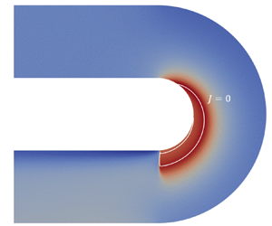
Non-ideal gasdynamic effects are now examined by simulating the supersonic flow evolution of siloxane MM, presented in figure 15. Thermodynamics is modelled through the improved Peng–Robinson–Stryjek–Vera equation of state in the polytropic form (see Van der Stelt, Nannan & Colonna Reference Van der Stelt, Nannan and Colonna2012), which is implemented directly in SU2. Also in this case, the flow acceleration in the inner part of the channel results in a shock wave at the end of the curve. The Mach number evolution exhibits the expected non-monotone behaviour both in the radial direction (figure 15b) and in the expansion along the internal wall (blue line in figure 15c). The flow in the channel never fully reaches planar radial equilibrium conditions, which are attained only close to the shock wave. Figure 15(b) compares the planar radial equilibrium profile from theory and CFD at  $\theta = 175^{\circ }$, showing a fairly good match between theory and simulations.

Figure 15. Supersonic Mach number evolution of MM in non-ideal conditions throughout the curved channel with Mach number at the inlet  $M_{in} = 0.5$: (a) Mach contours and $J=0$ line (white); (b) comparison between the radial profile from CFD at $\theta = 175^{\circ }$ and the theoretical planar radial equilibrium solution; (c) Mach evolution along the walls, compared with the equilibrium values. Reduced total conditions at the inlet are $P_{t}/P_{c}=2.08$ and $T_{t}/T_{c}=1.05$.
The numerical simulations confirm the flow evolution towards the planar radial equilibrium profile predicted by theory in the supersonic case. It is remarkable that, similarly to what was observed for subsonic flows, the achievement of a fully developed planar radial equilibrium condition is not guaranteed but instead depends on several parameters, such as the channel width and, for non-ideal flows, the fluid molecular complexity and stagnation conditions.
5. Conclusions
A relation for the Mach number dependency on the radius of curvature was presented for compressible flows in planar radial equilibrium. The ordinary differential equation was derived for a fluid governed by an arbitrary equation of state.
In the case of an ideal gas with constant specific heats, the equation was integrated analytically. A monotonically decreasing profile of the Mach number with the radius was found, and the dependence of the Mach profile on the molecular complexity of the fluids was discussed.
For thermodynamic states close to the liquid–vapour saturation curve and the critical point, the fluid gasdynamics departs from the ideal-gas solutions. Low molecular complexity fluid flows are qualitatively similar to those of ideal gases, and only quantitative differences are possible, termed non-ideal thermodynamic effects. In particular, the flow evolution along the radius shows a non-ideal dependence on total conditions, a well-known non-ideal thermodynamic effect. High molecular complexity fluids were shown to exhibit a non-monotone evolution of the Mach number with the radius in supersonic conditions, a non-ideal gasdynamic effect. For BZT fluids, non-monotone Mach number profiles were observed also in the subsonic regime.
The evolution of a uniform parallel flow towards planar radial equilibrium was studied by means of the streamline curvature method for subsonic flows, which also confirmed the prediction of the theory. Starting from a uniform parallel flow, the flow evolution towards planar radial equilibrium in a constant-curvature channel was characterised by increasing the ratio of the outer radius to the inner one in ideal flows, and by considering different stagnation conditions for non-ideal flows.
In the supersonic regime, flows developing through the same curved channel were analysed by means of inviscid CFD simulations, since a shock wave is observed in the inner part of the channel at the end of the curved duct. Upstream of the shock, the flow evolved isentropically towards the planar radial equilibrium condition predicted by the theory, eventually exhibiting non-ideal gasdynamic effects for high molecular complexity fluids.
Declaration of interests
The authors report no conflict of interest.
Appendix A. Analytical integration of the planar radial equilibrium equation for ideal gases
The analytical integration of the planar radial equilibrium equation for ideal gases (2.7) is reported in this appendix for completeness.
The differential equation reads
 \begin{equation} \frac{{\rm d}M}{{\rm d}\tilde{r}}={-} \frac{M}{\tilde{r}} \left(1+\frac{\gamma-1}{2}\,M^2 \right). \end{equation}
A rearrangement of the different terms leads to
 \begin{equation} \frac{{\rm d}M}{M \left(1+\dfrac{\gamma-1}{2}\,M^2 \right)} ={-}\frac{{\rm d}\tilde{r}}{\tilde{r}} \end{equation}
and then to
 \begin{equation} \frac{{\rm d}M}{M} - \frac{\dfrac{\gamma-1}{2}\,M}{1+\dfrac{\gamma-1}{2}\,M^2}\,{\rm d}M ={-}\frac{{\rm d} \tilde{r}}{\tilde{r}} . \end{equation}
The right-hand side is integrated between the dimensionless radius at the internal wall  $\tilde {r}_i$ and its generic value $\tilde {r}$. Analogously, the left-hand side is integrated between the Mach number at the internal wall $M_i$ and its generic value $M$. Note that, by definition, $\tilde {r}_i = r_i / r_i = 1$. The integration of the three terms yields
 $$\begin{gather} \int_{M_i}^{M} \frac{{\rm d}M}{M} - \int_{M_i}^{M} \frac{\dfrac{\gamma-1}{2}\,M}{1+\dfrac{\gamma-1}{2}\,M^2}\, {\rm d}M ={-} \int_{\tilde{r}_i}^{\tilde{r}} \frac{{\rm d}\tilde{r}}{\tilde{r}} , \end{gather}$$
 $$\begin{gather}\ln \left( \frac{M}{M_i} \right) - \frac{1}{2} \ln \left(\frac{1+\dfrac{\gamma-1}{2}\,M^2}{1+\dfrac{\gamma-1}{2}\,M_i^2} \right) ={-} \ln \tilde{r} . \end{gather}$$
By exploiting the properties of logarithms and performing additional computations, one can obtain the expressions
 \begin{equation} \ln \left( \frac{M}{M_i}\, \sqrt{\frac{1+\dfrac{\gamma-1}{2}\,M_i^2}{1+\dfrac{\gamma-1}{2}\,M^2}}\right) = \ln \left (\frac{1}{\tilde{r}} \right) \end{equation}
and
 \begin{equation} \frac{M^2 \left(1+\dfrac{\gamma-1}{2}\,M_i^2 \right)}{M_i^2 \left(1+\dfrac{\gamma-1}{2}\,M^2 \right)} = \frac{1}{\tilde{r}^2}. \end{equation}
Finally, rearranging the different terms leads to
 \begin{equation} \tilde{r}^2 M^2 \left(1+\frac{\gamma-1}{2}\,M_i^2 \right) = M_i^2 \left(1+\frac{\gamma-1}{2}\,M^2 \right), \end{equation}
which can be rewritten as
 \begin{equation} M^2 \left[ \left(1+\frac{\gamma-1}{2}\,M_i^2\right) \tilde{r}^2 - \frac{\gamma-1}{2}\,M_i^2\right] = M_i^2 , \end{equation}
yielding the final expression for the Mach number evolution along the non-dimensional radius,
 \begin{equation} M(\tilde{r})= \frac{M_i}{\sqrt{\left (1+\dfrac{\gamma-1}{2}\,M_i^2 \right ) \tilde{r}^2 - \dfrac{\gamma-1}{2}\,M_i^2}}, \end{equation}
reported in (2.8).


