


1. Introduction
This investigation explores the control of broad oceanic flows by rough topography, which is defined here as irregular bathymetric features with lateral scales of several kilometres. A series of recent modelling studies has demonstrated the profound impact of seafloor roughness on large-scale and mesoscale circulation patterns. For instance, small-scale variability in the bottom relief regulates the pattern and intensity of baroclinic instability in vertically sheared currents (e.g. LaCasce et al. Reference LaCasce, Escartin, Chassignet and Xu2019; Radko Reference Radko2020; Palóczy & LaCasce Reference Palóczy and LaCasce2022). Rough bathymetry can stabilize coherent vortices (Gulliver & Radko Reference Gulliver and Radko2022), extending their lifespan and enhancing their ability to transport heat, salt and nutrients. Even such major features of the ocean circulation as the Gulf Stream pathway and variability can be affected. Chassignet & Xu (Reference Chassignet and Xu2017) argue that the principal threshold for a significant improvement in the Gulf Stream representation in numerical models is an increase in the horizontal resolution to the submesoscale-enabled grid spacing. When spacing was decreased from 1/12° to 1/50° (~1.5 km at mid-latitudes), the simulated Gulf Stream and associated recirculating gyres transformed from unrealistic to realistic – the improvement attributed to a better representation of small-scale bathymetry.
While the general significance of seafloor roughness is no longer in doubt, our understanding of the specific physical mechanisms at play remains limited (Mashayek Reference Mashayek2023). For instance, considerable effort has been invested in analyses of the topographic pressure torque (Hughes & de Cuevas Reference Hughes and De Cuevas2001; Jackson, Hughes & Williams Reference Jackson, Hughes and Williams2006; Stewart, McWilliams & Solodoch Reference Stewart, McWilliams and Solodoch2021), with particular emphasis on lee-wave drag (Naveira Garabato et al. Reference Naveira Garabato, Nurser, Scott and Goff2013; Eden, Olbers & Eriksen Reference Eden, Olbers and Eriksen2021; Klymak et al. Reference Klymak, Balwada, Garabato and Abernathey2021). Less attention was paid to an alternative mechanism involving topographically induced Reynolds stresses. The interaction of broad abyssal currents with rough bathymetry inevitably generates small-scale eddies, and the associated eddy-induced transfer of momentum, in turn, influences primary flows. A recent analysis (Radko Reference Radko2023) suggests that the topographically induced Reynolds stresses control the abyssal circulation for moderately swift flows whereas the pressure torque becomes more significant for low velocities. However, more detailed investigations are required to determine the universality of these inferences. Even the sign of the effect cannot be assumed a priori. Generally, topographic forcing tends to substantially slow down large-scale abyssal currents (Gulliver & Radko Reference Gulliver and Radko2022, Reference Gulliver and Radko2023; Radko Reference Radko2022a,Reference Radkob). On the other hand, an argument can be made (Holloway Reference Holloway1987, Reference Holloway1992) that the interaction between topography and eddies can sometimes reinforce primary circulation patterns.
The lack of clear insight into the dynamics of flow–topography interaction – disconcerting as it is in its own right – also adversely impacts our ability to represent the effects of roughness in theoretical and coarse-resolution numerical models. Despite the continuous advancements in high-performance computing, roughness-resolving models will not be routinely used for global operational and climate simulations in the foreseeable future. Thus, parameterizing the effects of small-scale bathymetry is the most feasible way forward. A promising development in this area is the sandpaper theory (Radko Reference Radko2022a,Reference Radkob, Reference Radko2023; Gulliver & Radko Reference Gulliver and Radko2023; Mashayek Reference Mashayek2023), which attempts to evaluate the flow forcing by rough topography from the Fourier spectrum of the bottom relief. While small-scale seafloor patterns at different locations are as unique as our fingerprints, their spectral characteristics may be much more uniform. Thus, our focus on bathymetric spectra affords an appealing opportunity to develop rigorous universal parameterizations.
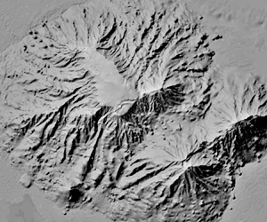
Although the sandpaper theory lays out the general roadmap for parameterizing the large-scale effects of roughness, much more work needs to be done. The key limitation of our earlier efforts is their focus on relatively calm environmental conditions. The first-generation sandpaper model (Radko Reference Radko2022a,Reference Radkob) was based on the quasi-geostrophic approximation, which assumes gentle topographic slopes and weak flows with low Rossby numbers. While these conditions are met in some regions, there are numerous locations in the World Ocean where quasi-geostrophy is inapplicable. A case in point is figure 1, which depicts the Atlantis II Seamount, an active area with complex bathymetry that has been the subject of recent extensive observational studies. The seafloor relief is dominated by a large-scale elevation with a lateral extent of ~100 km, perturbed by irregular patterns varying on the scale of kilometres. The ocean depth more than doubles from its value at the peak of the seamount to the depth at its base. This change violates one of the principal assumptions of the quasi-geostrophic approximation – the requirement for the depth variation to be much less than its reference value.

Figure 1. Complex multiscale terrain of the Atlantis II Seamount  $({38^ \circ }30^{\prime}N,\ {63^ \circ }10^{\prime}\textrm{W)}$.
The analysis of such challenging configurations demands the transition from the convenient but restrictive quasi-geostrophic (QG) approximation to a more general framework, capable of representing relatively steep topography and rapid flows. To this end, we formulate the next-generation sandpaper theory based on the governing shallow-water (SW) equations (e.g. Pedlosky Reference Pedlosky1987). The model is developed using conventional methods of multiscale homogenization mechanics (e.g. Manfroi & Young Reference Manfroi and Young1999, Reference Manfroi and Young2002; Balmforth & Young Reference Balmforth and Young2002, Reference Balmforth and Young2005; Mei & Vernescu Reference Mei and Vernescu2010). In the interest of tractability, the early attempts to apply multiscale techniques to flow–topography interaction problems assumed simple analytical small-scale patterns (e.g. Benilov Reference Benilov2000, Reference Benilov2001; Vanneste Reference Vanneste2000, Reference Vanneste2003; Radko Reference Radko2020; Goldsmith & Esler Reference Goldsmith and Esler2021). The drawback of these models is the inherent qualitative connection of the resulting solutions to oceanic systems, which are characterized by highly irregular seafloor patterns (e.g. figure 1). Fortunately, as was noted by Radko (Reference Radko2022a,Reference Radkob), analytical progress can still be made for irregular bathymetry, provided that its spectrum is known. The crux of the proposed technique is the application of Parseval's theorem (Parseval Reference Parseval1806), which relates the spatial averages of quadratic quantities to their Fourier spectra. The explicit and statistically accurate bathymetric spectrum of Goff & Jordan (Reference Goff and Jordan1988) proved to be well suited for the proposed approach, leading to a closed set of large-scale evolutionary equations (Radko Reference Radko2022a,Reference Radkob, Reference Radko2023).
The present study shows that the transition from the QG to SW framework is relatively straightforward and does not require a major revision of methodology. The SW-based formulation of the sandpaper theory reduces to its QG counterpart in the limit of low Rossby numbers and weak variation in the seafloor depth. To assess the performance characteristics of the resulting parameterization, we consider the interaction of an externally forced flow with a corrugated seamount – the configuration illustrated in figure 2. The parametric simulations based on the SW sandpaper theory are compared with the corresponding roughness-resolving simulations. The close agreement between the two indicates that the updated sandpaper model can accurately represent active systems with relatively large Rossby numbers and substantial depth variation.

Figure 2. Schematic diagram illustrating the setup of validation experiments for the SW sandpaper model. An externally forced current interacts with a large-scale seamount, which is represented by the Gaussian pattern (blue curve) perturbed by irregular small-scale variability (black curve).
The material is organized as follows. The governing equations are described in § 2. Section 3 presents the asymptotic multiscale theory that leads to an explicit parameterization of the large-scale effects of seafloor roughness. The analytical model is validated by simulations in § 4. The results are summarized, and conclusions are drawn, in § 5.
2. Formulation
Consider a homogeneous incompressible flow represented by the SW model (e.g. Pedlosky Reference Pedlosky1987). The momentum equations take the form
 \begin{equation}\left. {\begin{array}{*{20}{c@{}}} {\dfrac{{\partial {u^ \ast }}}{{\partial {t^\ast }}} + {u^\ast }\dfrac{{\partial {u^ \ast }}}{{\partial {x^\ast }}} + {v^\ast }\dfrac{{\partial {u^ \ast }}}{{\partial {y^\ast }}} - {f^\ast }{v^\ast } =- \dfrac{1}{{\rho_0^\ast }}\dfrac{{\partial {p^\ast }}}{{\partial {x^\ast }}} + {\upsilon^\ast }{\nabla^2}{u^\ast }}\\ {\dfrac{{\partial {v^ \ast }}}{{\partial {t^\ast }}} + {u^\ast }\dfrac{{\partial {v^ \ast }}}{{\partial {x^\ast }}} + {v^\ast }\dfrac{{\partial {v^ \ast }}}{{\partial {y^\ast }}} + {f^\ast }{u^\ast } =- \dfrac{1}{{\rho_0^\ast }}\dfrac{{\partial {p^\ast }}}{{\partial {y^\ast }}} + {\upsilon^\ast }{\nabla^2}{v^\ast }} \end{array}} \right\},\end{equation}
where  $({u^\ast },{v^\ast })$ are the lateral velocity components, which are assumed to be vertically uniform, ${p^\ast }$ is pressure, $\rho _0^\ast $ is the density, ${\upsilon ^\ast }$ is the eddy viscosity and ${f^\ast }$ is the Coriolis parameter. The asterisks represent dimensional quantities.
The following model ignores the bottom Ekman friction. This choice is motivated by (i) the considerations of simplicity and dynamic transparency and (ii) our experience with the previous version of the sandpaper model (Radko Reference Radko2022a,Reference Radkob). Those earlier analyses suggest that the Ekman dynamics plays a secondary role in topographic control for typical oceanic conditions. We also adopt the rigid-lid approximation for the sea surface, which is a common and widely accepted simplification for large-scale and mesoscale ocean models (e.g. Pedlosky Reference Pedlosky1987; Vallis Reference Vallis2006). The rigid-lid approximation assumes that vertical velocity is zero at the still-water level, simplifying the thickness equation to
 \begin{equation}\frac{\partial }{{\partial {x^\ast }}}({u^\ast }{h^\ast }) + \frac{\partial }{{\partial {y^\ast }}}({v^\ast }{h^\ast }) = 0,\end{equation}
where  ${h^\ast }$ is the local ocean depth. To reduce the number of controlling parameters, governing equations are non-dimensionalized as follows:
 \begin{equation}({u^\ast },{v^\ast }) = f_0^\ast {L^\ast }(u,v),\quad ({x^\ast },{y^\ast }) = {L^\ast }(x,y),\quad {t^\ast } = \frac{t}{{f_0^\ast }},\quad {h^\ast } = {H^\ast }h,\end{equation}
where  ${L^\ast }$, ${H^\ast }$ and $f_0^\ast $ are the representative scales for the width of small-scale topographic features, the ocean depth and the Coriolis parameter, respectively. To be specific, we consider the oceanographically relevant scales of
 \begin{equation}{L^\ast } = {10^4}\ \textrm{m},\quad {H^\ast } = 4000\ \textrm{m},\quad f_0^\ast= {10^{ - 4}}\ \textrm{s}{}^{ - 1}.\end{equation}
The governing system is simplified further by taking the curl of the momentum equations (2.1), which eliminates the pressure gradient terms and yields the vorticity equation
 \begin{equation}\frac{{\partial \varsigma }}{{\partial t}} + u\frac{{\partial {\varsigma _a}}}{{\partial x}} + v\frac{{\partial {\varsigma _a}}}{{\partial y}} + {\varsigma _a}\left( {\frac{{\partial u}}{{\partial x}} + \frac{{\partial v}}{{\partial y}}} \right) = \upsilon {\nabla ^2}\varsigma ,\end{equation}
where
 \begin{equation}\varsigma = \frac{{\partial v}}{{\partial x}} - \frac{{\partial u}}{{\partial y}},\quad {\varsigma _a} = \varsigma + f.\end{equation}
Combining (2.5) and (2.2), we reduce the vorticity equation to
 \begin{equation}\frac{{\partial \varsigma }}{{\partial t}} + uh\frac{{\partial q}}{{\partial x}} + vh\frac{{\partial q}}{{\partial y}} = \upsilon {\nabla ^2}\varsigma ,\end{equation}
where q is the potential vorticity
 \begin{equation}q = \frac{{f + \varsigma }}{h}.\end{equation}
 Equation (2.2) implies that the volume transport is non-divergent, and therefore it is conveniently represented by the transport streamfunction  $(\psi )$
 \begin{equation}uh =- \frac{{\partial \psi }}{{\partial y}},\quad vh = \frac{{\partial \psi }}{{\partial x}}.\end{equation}
This, in turn, casts the problem in the vorticity–streamfunction form
 \begin{equation}\frac{{\partial \varsigma }}{{\partial t}} + J(\psi ,q) = \upsilon {\nabla ^2}\varsigma ,\end{equation}
where J is the Jacobian, and
 \begin{equation}\varsigma = \frac{\partial }{{\partial x}}\left( {\frac{1}{h}\frac{{\partial \psi }}{{\partial x}}} \right) + \frac{\partial }{{\partial y}}\left( {\frac{1}{h}\frac{{\partial \psi }}{{\partial y}}} \right).\end{equation}
To explore the interaction between flow components of large and small lateral extents, we introduce the scale-separation parameter
 \begin{equation}\varepsilon = \frac{{{L_C}}}{{{L_{LS}}}} \ll 1,\end{equation}
where  ${L_{LS}}$ is the representative lateral extent of the large-scale flow, and ${L_C}$ is the cutoff value that separates scales that we intend to resolve from those that we wish to parameterize. Parameter $\varepsilon $ is used to define the new set of spatial scales $(X,Y)$ that reflects the dynamics of large-scale processes. These variables are related to the original ones through
 \begin{equation}(X,Y) = \varepsilon (x,y).\end{equation}
The derivatives in the governing system (2.5) are replaced accordingly
 \begin{equation}\frac{\partial }{{\partial x}} \to \frac{\partial }{{\partial x}} + \varepsilon \frac{\partial }{{\partial X}},\quad \frac{\partial }{{\partial y}} \to \frac{\partial }{{\partial y}} + \varepsilon \frac{\partial }{{\partial Y}}.\end{equation}
 The variation in depth  $\eta = H - h$ contains both large and small scales
 \begin{equation}\eta = {\eta _L}(X,Y) + {\eta _S}(x,y).\end{equation}
A natural way to separate bathymetry into the small- and large-scale components (Radko Reference Radko2022a,Reference Radkob) is based on the Fourier transform of  $\eta $
 \begin{equation}\eta = \frac{{\sqrt {{L_x}{L_y}} }}{{2{\rm \pi}}}\iint {\tilde{\eta }(k,l){\rm exp} (\textrm{i}kx + \textrm{i}ly)\,\textrm{d}k\,\textrm{d}l} ,\end{equation}
where  $(k,l)$ are the wavenumbers in x and y, respectively, tildes hereafter denote Fourier images and $({L_x},{L_y})$ is the domain size. Since the Fourier transform is linear, it can be conveniently separated into the contributions from high and low wavenumbers as follows:
 \begin{align}\eta = \underbrace{{\frac{{\sqrt {{L_x}{L_y}} }}{{2{\rm \pi}}}\iint\limits_{\kappa < 2{\rm \pi}/{L_C}} {\tilde{\eta }(k,l){\rm exp} (\textrm{i}kx + \textrm{i}ly)\,\textrm{d}k\,\textrm{d}l} }}_{{{\eta _L}}} + \underbrace{{\frac{{\sqrt {{L_x}{L_y}} }}{{2{\rm \pi}}}\iint\limits_{\kappa > 2{\rm \pi}/{L_C}} {\tilde{\eta }(k,l){\rm exp} (\textrm{i}kx + \textrm{i}ly)\,\textrm{d}k\,\textrm{d}l} }}_{{{\eta _S}}},\end{align}
where  $\kappa \equiv \sqrt {{k^2} + {l^2}} $. The ${\eta _L}$ component in (2.17) gently varies on relatively large scales, and ${\eta _S}$ represents small-scale variability. The normalization factor $\sqrt {{L_x}{L_y}} /2{\rm \pi}$ in the definition of Fourier transform is introduced to ensure that the Parseval identity (Parseval Reference Parseval1806), to be used in subsequent developments, takes a convenient form
 \begin{equation}{\langle ab\rangle _{x,y}} = \iint {\tilde{a} \cdot conj(\tilde{b})\,\textrm{d}k\,\textrm{d}l} .\end{equation}
Angle brackets hereafter represent mean values, with the averaging variables listed in the subscript.
3. The multiscale analysis
We now proceed with the development of large-scale evolutionary equations for system (2.10) using methods of multiscale mechanics (e.g. Mei & Vernescu Reference Mei and Vernescu2010). Our earlier explorations (Radko Reference Radko2023) revealed that the dynamics of flow–topography interactions differs substantially for relatively slow and swift flows. While this result was obtained using the QG-based model, it guides the analytical treatment of SW systems as well. Thus, we separately consider the asymptotic limits of high and low Reynolds numbers (Re), defined here as
 \begin{equation}Re = \frac{{{U^\ast }{L^\ast }}}{{{\upsilon ^\ast }}},\end{equation}
where  ${U^\ast }$ is the representative large-scale velocity. The ultimate objective is the development of a universal large-scale model that effectively bridges the two limits.
3.1. Fast flows
To describe the weakly dissipative limit of  $Re \to \infty $, we consider the asymptotic sector $U = O(1)$ and $\upsilon = O(\varepsilon )$, which corresponds to $Re = O({\varepsilon ^{ - 1}})$. The complication that one encounters in treating this limit is the presence of two dissimilar evolutionary time scales set by relatively fast advective processes $({t_1} = \varepsilon t)$ and much slower dissipative effects $({t_3} = {\varepsilon ^3}t)$. To capture both evolutionary patterns, we replace the time derivative in the governing system (2.10) by
 \begin{equation}\frac{\partial }{{\partial t}} \to \varepsilon \frac{\partial }{{\partial {t_1}}} + {\varepsilon ^3}\frac{\partial }{{\partial {t_3}}}.\end{equation}
We open expansion with the order-one large-scale flow
 \begin{equation}\left. {\begin{array}{*{20}{c@{}}} {u = {u_0}(X,Y,{t_1},{t_3}) + \varepsilon {u_1}(X,Y,x,y,{t_1},{t_3}) + {\varepsilon^2}{u_2}(X,Y,x,y,{t_1},{t_3}) + \cdots }\\ {v = {v_0}(X,Y,{t_1},{t_3}) + \varepsilon {v_1}(X,Y,x,y,{t_1},{t_3}) + {\varepsilon^2}{v_2}(X,Y,x,y,{t_1},{t_3}) + \cdots } \end{array}} \right\},\end{equation}
which demands that the streamfunction takes the form
 \begin{align}\psi = {\varepsilon ^{ - 1}}{\psi _{ - 1}}(X,Y,{t_1},{t_3}) + \varepsilon {\psi _1}(X,Y,x,y,{t_1},{t_3}) + {\varepsilon ^2}{\psi _2}(X,Y,x,y,{t_1},{t_3}) + \cdots ,\end{align}
and the analogous notation is used for q and  $\varsigma $ series. The eddy viscosity and small-scale bathymetric variability are rescaled as follows:
 \begin{equation}\upsilon = \varepsilon {\upsilon _0},\quad {\eta _S} = \varepsilon {\eta _{S0}}.\end{equation}
Importantly, the large-scale depth variation is treated as an order-one quantity:  ${h_L}(X,Y) = 1 - {\eta _L}(X,Y)$. The Coriolis parameter $f = f(Y)$ is a function of the large-scale latitudinal coordinate only.
Series (3.3) are substituted in (2.10) and terms of the same order are collected. The leading-order balance of the vorticity equation is realized at  $O(\varepsilon )$
 \begin{equation}\frac{{\partial {\psi _{ - 1}}}}{{\partial X}}\frac{{\partial {q_1}}}{{\partial y}} - \frac{{\partial {\psi _{ - 1}}}}{{\partial Y}}\frac{{\partial {q_1}}}{{\partial x}} + {J_{X,Y}}({\psi _{ - 1}},{q_0}) = 0.\end{equation}
Averaging (3.6) in  $(x,y)$ leads to
 \begin{equation}{J_{X,Y}}({\psi _{ - 1}},{q_0}) = 0,\end{equation}
where  ${q_0} \equiv f/{h_L}$ and ${J_{X,Y}}$ denotes the Jacobian in large-scale variables
 \begin{equation}{J_{X,Y}}(a,b) \equiv \frac{{\partial a}}{{\partial X}}\frac{{\partial b}}{{\partial Y}} - \frac{{\partial a}}{{\partial Y}}\frac{{\partial b}}{{\partial X}}.\end{equation}
Equation (3.7) reflects the so-called topographic steering effect – the tendency of large-scale flows to follow the contours of  $f/{h_L}$ (e.g. Marshall Reference Marshall1995; Wåhlin Reference Wåhlin2002). However, when (3.6) and (3.7) are subtracted, we are also met with the demand to comply with
 \begin{equation}\frac{{\partial {\psi _{ - 1}}}}{{\partial X}}\frac{{\partial {q_1}}}{{\partial y}} - \frac{{\partial {\psi _{ - 1}}}}{{\partial Y}}\frac{{\partial {q_1}}}{{\partial x}} = 0.\end{equation}
This condition is satisfied by insisting that the first-order potential vorticity perturbation does not vary on small spatial scales
 \begin{equation}{q_1} = {q_1}(X,Y,{t_1},{t_3}).\end{equation}
Statement (3.10) reflects the tendency for small-scale homogenization of potential vorticity. Homogenization controls the dynamics of numerous geophysical systems (e.g. Rhines & Young Reference Rhines and Young1982; Dewar Reference Dewar1986; Marshall, Williams & Lee Reference Marshall, Williams and Lee1999) and it spectacularly manifested itself in our previous studies of flow–topography interaction (Radko Reference Radko2022a,Reference Radkob, Reference Radko2023; Gulliver & Radko Reference Gulliver and Radko2023). The lack of small-scale variability in the first-order potential vorticity field implies that the rapid increase (decrease) in the fluid depth is compensated by the corresponding increase (decrease) in relative vorticity
 \begin{equation}{\varsigma _1} = {\langle {\varsigma _1}\rangle _{x,y}} - \frac{f}{{{h_L}}}{\eta _{S0}}.\end{equation}
Equation (3.11), in turn, leads to
 \begin{equation}{\nabla ^2}{\psi _1} =- \frac{1}{{{h_L}}}\left( {\frac{{\partial {\psi_{ - 1}}}}{{\partial X}}\frac{{\partial {\eta_{S0}}}}{{\partial x}} + \frac{{\partial {\psi_{ - 1}}}}{{\partial Y}}\frac{{\partial {\eta_{S0}}}}{{\partial y}}} \right) - f{\eta _{S0}}.\end{equation}
The second-order balance reveals an even more interesting dynamics
 \begin{align}\frac{{\partial {\varsigma _1}}}{{\partial {t_1}}} + \frac{{\partial {\psi _1}}}{{\partial x}}\frac{{\partial {q_0}}}{{\partial Y}} - \frac{{\partial {\psi _1}}}{{\partial y}}\frac{{\partial {q_0}}}{{\partial X}} + \frac{{\partial {\psi _{ - 1}}}}{{\partial X}}\frac{{\partial {q_2}}}{{\partial y}} - \frac{{\partial {\psi _{ - 1}}}}{{\partial Y}}\frac{{\partial {q_2}}}{{\partial x}} + {J_{X,Y}}({\psi _{ - 1}},{q_1}) = {\upsilon _0}{\nabla ^2}{\varsigma _1}.\end{align}
When (3.13) is averaged in  $(x,y)$, we arrive at
 \begin{equation}\frac{{\partial {{\langle {\varsigma _1}\rangle }_{x,y}}}}{{\partial {t_1}}} + {J_{X,Y}}({\psi _{ - 1}},{q_1}) = 0,\end{equation}
which essentially represents the leading-order Lagrangian conservation of large-scale potential vorticity. However, when (3.14) and (3.13) are subtracted, we arrive, using (3.11), at
 \begin{equation}\frac{{\partial {\psi _1}}}{{\partial x}}\frac{{\partial {q_0}}}{{\partial Y}} - \frac{{\partial {\psi _1}}}{{\partial y}}\frac{{\partial {q_0}}}{{\partial X}} + \frac{{\partial {\psi _{ - 1}}}}{{\partial X}}\frac{{\partial {q_2}}}{{\partial y}} - \frac{{\partial {\psi _{ - 1}}}}{{\partial Y}}\frac{{\partial {q_2}}}{{\partial x}} = {\upsilon _0}\frac{f}{{{h_L}}}{\nabla ^2}{\eta _{S0}},\end{equation}
which connects the small-scale variability in potential vorticity  $({q_2})$ to the roughness pattern $({\eta _{S0}})$.
The analysis of the  $O({\varepsilon ^3})$ balance proves to be somewhat uneventful. For future use, we list its $(x,y)$ average
 \begin{equation}\frac{{\partial {{\left\langle {{\varsigma_2}} \right\rangle }_{x,y}}}}{{\partial {t_1}}} + {J_{X,Y}}({\langle {\psi _1}\rangle _{x,y}},{q_0}) + {J_{X,Y}}({\psi _{ - 1}},{\langle {q_2}\rangle _{x,y}}) = 0.\end{equation}
The key solvability condition that leads to the evolutionary large-scale model is obtained by averaging the  $O({\varepsilon ^4})$ balance in x and y
 \begin{align}\frac{{\partial
{{\langle {\varsigma _1}\rangle }_{x,y}}}}{{\partial
{t_3}}} &+ \frac{{\partial {{\langle {\varsigma _3}\rangle
}_{x,y}}}}{{\partial {t_1}}} + {J_{X,Y}}({\psi _{ -
1}},{\langle {q_3}\rangle _{x,y}}) + {J_{X,Y}}({\langle
{\psi _1}\rangle _{x,y}},{q_1}) + {J_{X,Y}}({\langle {\psi
_2}\rangle _{x,y}},{q_0})\notag\\ &+ {D_{fast\;0}} = {\upsilon
_0}\nabla _{X,Y}^2{\langle {\varsigma _1}\rangle
_{x,y}},\end{align}
\begin{align}\frac{{\partial
{{\langle {\varsigma _1}\rangle }_{x,y}}}}{{\partial
{t_3}}} &+ \frac{{\partial {{\langle {\varsigma _3}\rangle
}_{x,y}}}}{{\partial {t_1}}} + {J_{X,Y}}({\psi _{ -
1}},{\langle {q_3}\rangle _{x,y}}) + {J_{X,Y}}({\langle
{\psi _1}\rangle _{x,y}},{q_1}) + {J_{X,Y}}({\langle {\psi
_2}\rangle _{x,y}},{q_0})\notag\\ &+ {D_{fast\;0}} = {\upsilon
_0}\nabla _{X,Y}^2{\langle {\varsigma _1}\rangle
_{x,y}},\end{align}
where  $\nabla _{X,Y}^2 \equiv {\partial ^2}/\partial {X^2} + {\partial ^2}/\partial {Y^2}$ and
 \begin{equation}{D_{fast\;0}} = \frac{\partial }{{\partial X}}{\left\langle {{\psi_1}\frac{{\partial {q_2}}}{{\partial y}}} \right\rangle _{x,y}} - \frac{\partial }{{\partial Y}}{\left\langle {{\psi_1}\frac{{\partial {q_2}}}{{\partial x}}} \right\rangle _{x,y}}.\end{equation}
We now combine all  $(x,y)$ averaged equations, which include (3.7), (3.14), (3.16) and (3.17). The resulting evolutionary equation is simplified by introducing the large-scale streamfunction
 \begin{equation}\bar{\psi } = {\varepsilon ^{ - 1}}{\psi _{ - 1}} + \varepsilon {\langle {\psi _1}\rangle _{x,y}} + {\varepsilon ^2}{\langle {\psi _2}\rangle _{x,y}},\end{equation}
the corresponding large-scale vorticity
 \begin{equation}\bar{\varsigma } = {\varepsilon ^2}\frac{\partial }{{\partial X}}\left( {\frac{1}{{{h_L}}}\frac{{\partial \bar{\psi }}}{{\partial X}}} \right) + {\varepsilon ^2}\frac{\partial }{{\partial Y}}\left( {\frac{1}{{{h_L}}}\frac{{\partial \bar{\psi }}}{{\partial Y}}} \right),\end{equation}
and potential vorticity
 \begin{equation}\bar{q} = \frac{{f + \bar{\varsigma }}}{{{h_L}}}.\end{equation}
Using (3.19)–(3.21) and neglecting all  $o({\varepsilon ^4})$ components, we express the large-scale evolutionary equation in terms of $\textrm{(}\bar{\varsigma },\bar{\psi },\bar{q}\textrm{)}$
 \begin{equation}\varepsilon \frac{{\partial \bar{\varsigma }}}{{\partial {t_1}}} + {\varepsilon ^3}\frac{{\partial \bar{\varsigma }}}{{\partial {t_3}}} + {\varepsilon ^2}{J_{X,Y}}(\bar{\psi },\bar{q}) + {\varepsilon ^4}{D_{fast\;0}} = {\varepsilon ^3}{\upsilon _0}\nabla _{X,Y}^2\bar{\varsigma }.\end{equation}
Equation (3.22) is written exclusively in terms of large-scale independent variables  $\textrm{(}X\textrm{,}Y\textrm{,}{t_1}\textrm{,}{t_3}\textrm{)}$. Thus, at this point, we can revert to their original counterparts $(x,y,t)$ without the risk of confusing the scales
 \begin{equation}\left. {\begin{array}{*{20}{c@{}}} {\dfrac{\partial }{{\partial t}}\bar{\varsigma } + J(\bar{\psi },\bar{q}) + {D_{fast}} = \upsilon {\nabla^2}\bar{\varsigma }}\\ {\bar{\varsigma } = \dfrac{\partial }{{\partial x}}\left( {\dfrac{1}{{{h_L}}}\dfrac{{\partial \bar{\psi }}}{{\partial x}}} \right) + \dfrac{\partial }{{\partial y}}\left( {\dfrac{1}{{{h_L}}}\dfrac{{\partial \bar{\psi }}}{{\partial y}}} \right)} \end{array}} \right\},\end{equation}
where  ${D_{fast}} = {\varepsilon ^4}{D_{fast\;0}}$. The large-scale equations (3.21) and (3.23) are structurally analogous to the original system (2.8), (2.10), and (2.11). Their significance lies in the ability to isolate and consistently describe the motion of large-scale flow components. The cumulative effect of the small-scale variability is represented solely by the forcing term $({D_{fast}})$ in the vorticity equation. To close the system, we express ${D_{fast}}$ in terms of properties of the large-scale flow by eliminating ${q_2}$ in (3.18) using (3.15). This procedure is described in Appendix A, and the result is
 \begin{equation}{D_{fast}} = \frac{\partial }{{\partial x}}\left( {{G_{fast}}\frac{{\bar{v}}}{{{{\bar{V}}^2}}}} \right) - \frac{\partial }{{\partial y}}\left( {{G_{fast}}\frac{{\bar{u}}}{{{{\bar{V}}^2}}}} \right),\quad {G_{fast}} = 2{\rm \pi}\upsilon \frac{{{f^2}}}{{h_L^2}}\int {|{{\tilde{\eta }}_S}{|^2}\kappa \,\textrm{d}\kappa } ,\end{equation}
where  $\bar{V} = \sqrt {{{\bar{u}}^2} + {{\bar{v}}^2}} $ is the absolute velocity.
3.2. Slow flows
While the foregoing model (§ 3.1) offers an explicit description of large-scale forcing by rough topography, its implementation in theoretical and coarse-resolution numerical models is hampered by the unbounded increase of (3.24a,b) in the weak flow limit:  $\bar{V} \to 0$. This singularity implies that relatively slow flows operate in a physically dissimilar regime. The dynamics of such systems is now captured by considering the strongly dissipative limit of $Re \ll 1$. To be specific, we explore the asymptotic sector $U = O({\varepsilon ^2})$ and $\upsilon = O(\varepsilon )$, which implies that $Re = O(\varepsilon )$. Anticipating that the evolution of large-scale patterns in this regime is controlled by slow frictional processes, the temporal variable is rescaled as ${t_3} = {\varepsilon ^3}t$. The time derivative in the governing system (2.10) is replaced accordingly
 \begin{equation}\frac{\partial }{{\partial t}} \to {\varepsilon ^3}\frac{\partial }{{\partial {t_3}}}.\end{equation}
We open the expansion with the leading-order large-scale flow
 \begin{equation}\left. {\begin{array}{*{20}{c@{}}} {u = {\varepsilon^2}{u_2}(X,Y,{t_3}) + {\varepsilon^3}{u_3}(X,Y,x,y,{t_3}) + {\varepsilon^4}{u_4}(X,Y,x,y,{t_3}) + \cdots }\\ {v = {\varepsilon^2}{v_2}(X,Y,{t_3}) + {\varepsilon^3}{v_3}(X,Y,x,y,{t_3}) + {\varepsilon^4}{v_4}(X,Y,x,y,{t_3}) + \cdots } \end{array}} \right\},\end{equation}
and the corresponding streamfunction pattern takes the form
 \begin{equation}\psi = \varepsilon {\psi _1}(X,Y,{t_3}) + {\varepsilon ^3}{\psi _3}(X,Y,x,y,{t_3}) + {\varepsilon ^4}{\psi _4}(X,Y,x,y,{t_3}) + \cdots .\end{equation}
The potential and relative vorticities (q and  $\varsigma $) are expanded similarly. The eddy viscosity and small-scale bathymetric variability are rescaled as follows:
 \begin{equation}\upsilon = \varepsilon {\upsilon _0},\quad {\eta _S} = {\varepsilon ^2}{\eta _{S0}}.\end{equation}
 The series (3.26) and (3.27) are substituted in the governing equations (2.10) and the terms of the same order are collected. The leading order balance of the vorticity equation is realized at  $O({\varepsilon ^3})$
 \begin{equation}{J_{X,Y}}({\psi _1},{q_0}) = 0.\end{equation}
Equation (3.29) reflects the topographic steering of large-scale flows. In this regard, the leading-order balance is analogous to (3.7) – its counterpart for fast flows. The  $O({\varepsilon ^4})$ balance of the vorticity equation amounts to
 \begin{equation}\frac{{\partial {\psi _1}}}{{\partial X}}\frac{{\partial {q_2}}}{{\partial y}} - \frac{{\partial {\psi _1}}}{{\partial Y}}\frac{{\partial {q_2}}}{{\partial x}} = {\upsilon _0}{\nabla ^2}{\varsigma _3} - \left( {\frac{{\partial {\psi_3}}}{{\partial x}}\frac{{\partial {q_0}}}{{\partial Y}} - \frac{{\partial {\psi_3}}}{{\partial y}}\frac{{\partial {q_0}}}{{\partial X}}} \right),\end{equation}
where
 \begin{equation}{q_2} = \frac{{f{\eta _{S0}}}}{{h_L^2}}.\end{equation}
The third-order component of relative vorticity  $({\varsigma _3})$ in (3.30) is expressed in terms of the streamfunction using (2.11)
 \begin{equation}{\varsigma _3} = \frac{{{\nabla ^2}{\psi _3}}}{{{h_L}}} + \frac{\partial }{{\partial X}}\left( {\frac{1}{{{h_L}}}\frac{{\partial {\psi_1}}}{{\partial X}}} \right) + \frac{\partial }{{\partial Y}}\left( {\frac{1}{{{h_L}}}\frac{{\partial {\psi_1}}}{{\partial Y}}} \right).\end{equation}
Recalling that  ${\psi _1}$ and ${h_L}$ vary only on large scales (X,Y), we conclude that the two last terms on the right-hand side of this equation do not depend on (x,y). Therefore, they are eliminated by applying the small-scale Laplacian to both sides of (3.32)
 \begin{equation}{\nabla ^2}{\varsigma _3} = \frac{{{\nabla ^4}{\psi _3}}}{{{h_L}}}.\end{equation}
Our theory also makes use of the small-scale average of the balance realized at  $O({\varepsilon ^5})$
 \begin{equation}{J_{X,Y}}({\langle {\psi _3}\rangle _{xy}},{q_0}) = 0.\end{equation}
The key solvability condition that represents the temporal variability of the large-scale flow is obtained by averaging the  $O({\varepsilon ^6})$ balance in x and y
 \begin{equation}\frac{{\partial {{\langle {\varsigma _3}\rangle }_{x,y}}}}{{\partial {t_3}}} + {J_{X,Y}}({\langle {\psi _4}\rangle _{x,y}},{q_0}) + {J_{X,Y}}({\psi _1},{\langle {q_3}\rangle _{x,y}}) + {D_{slow\;0}} = {\upsilon _0}\nabla _{X,Y}^2{\langle {\varsigma _3}\rangle _{x,y}},\end{equation}
where
 \begin{equation}{D_{slow\;0}} = \frac{\partial }{{\partial X}}{\left\langle {{\psi_3}\frac{{\partial {q_2}}}{{\partial y}}} \right\rangle _{x,y}} - \frac{\partial }{{\partial Y}}{\left\langle {{\psi_3}\frac{{\partial {q_2}}}{{\partial x}}} \right\rangle _{x,y}}.\end{equation}
To formulate the sought-after evolutionary equation, we now combine (3.29), (3.34) and (3.35) as follows:
 \begin{equation}\begin{array}{ccccc} & {\varepsilon ^6}\dfrac{{\partial {{\langle {\varsigma _3}\rangle }_{x,y}}}}{{\partial {t_3}}} + {\varepsilon ^3}{J_{X,Y}}({\psi _1},{q_0}) + {\varepsilon ^5}{J_{X,Y}}({\langle {\psi _3}\rangle _{x,y}},{q_0}) + {\varepsilon ^6}{J_{X,Y}}({\langle {\psi _4}\rangle _{x,y}},{q_0})\\ & \quad + \,{\varepsilon ^6}{J_{X,Y}}({\psi _1},{\langle {q_3}\rangle _{x,y}}) + {\varepsilon ^6}{D_{slow\;0}} = {\varepsilon ^6}{\upsilon _0}\nabla _{X,Y}^2{\langle {\varsigma _3}\rangle _{x,y}}. \end{array}\end{equation}
This expression is simplified by introducing the large-scale streamfunction
 \begin{equation}\bar{\psi } = \varepsilon {\psi _1} + {\varepsilon ^3}{\langle {\psi _3}\rangle _{x,y}} + {\varepsilon ^4}{\langle {\psi _4}\rangle _{x,y}},\end{equation}
and analogous quantities  $\bar{\varsigma }$ and $\bar{q}$ based on relative and potential vorticities. Neglecting all terms $o({\varepsilon ^6})$ reduces (3.37) to
 \begin{equation}{\varepsilon ^3}\frac{{\partial \bar{\varsigma }}}{{\partial {t_3}}} + {\varepsilon ^2}{J_{X,Y}}(\bar{\psi },\bar{q}) + {\varepsilon ^6}{D_{slow\;0}} = {\varepsilon ^3}{\upsilon _0}\nabla _{X,Y}^2\bar{\varsigma }.\end{equation}
Thus, we obtained the evolutionary equation (3.39) written exclusively in terms of large-scale independent variables  $(X,Y,{t_3})$. We now revert to the original variables $(x,y,t)$
 \begin{equation}\frac{\partial }{{\partial t}}\bar{\varsigma } + J(\bar{\psi },\bar{q}) + {D_{slow}} = \upsilon {\nabla ^2}\bar{\varsigma },\end{equation}
where  ${D_{slow}} = {\varepsilon ^6}{D_{slow\;0}}$. To close the system, it only remains to express ${D_{slow}}$ in terms of characteristics of the large-scale flow. To accomplish this task, we use (3.30) to eliminate ${q_2}$ in (3.36). The details are relegated to Appendix B, and the result is
 \begin{align}{D_{slow}} = \frac{\partial }{{\partial x}}({G_{slow}}\bar{v}) - \frac{\partial }{{\partial y}}({G_{slow}}\bar{u}),\quad {G_{slow}} = \frac{{2{\rm \pi}}}{\upsilon }\frac{{{f^2}}}{{h_L^2}}\int {\frac{{(\sqrt {1 + \delta } - 1)}}{{\delta \sqrt {1 + \delta } }}\frac{{|{{\tilde{\eta }}_S}{|^2}}}{\kappa }\,} \textrm{d}\kappa ,\end{align}
where  $\delta = {(({h_L}/\upsilon {\kappa ^3})|\boldsymbol{\nabla }{q_0}|)^2}$ and $(\bar{u},\bar{v}) = (1/{h_L})( - (\partial \bar{\psi }/\partial y),(\partial \bar{\psi }/\partial x))$. Our numerical simulations (not shown) reveal that the effects associated with $\delta $ tend to be very weak. If simplicity is desired, the expression for ${G_{slow}}$ in (3.41a,b) can be reduced to ${G_{slow}} = ({\rm \pi}/\upsilon )(\,{f^2}/h_L^2)\int {(|{{\tilde{\eta }}_S}{|^2}/\kappa )\,\textrm{d}\kappa }$ by taking the $\delta \to 0$ limit.
3.3. Hybrid model
The expressions for large-scale forcing by small-scale topography obtained for fast (§ 3.1) and slow (§ 3.2) flows are fundamentally different. For instance,  ${D_{slow}}$ tends to increase with increasing velocity, whereas ${D_{fast}}$ somewhat counterintuitively decreases. Such dramatic dissimilarity motivates the development of an explicit hybrid model that would seamlessly connect these asymptotic limits. The benefit of this effort is the roughness parameterization that could be readily implemented in course-resolution models.
In developing the hybrid model, we follow the approach suggested by Radko (Reference Radko2023). First, we note that forcing terms  ${D_{slow}}$ and ${D_{fast}}$ can both be written as
 \begin{equation}D = curl(\boldsymbol{M}),\end{equation}
where M represents the topographic momentum forcing. In the fast and slow limits,  $\boldsymbol{M}$ takes the following forms:
 \begin{equation}{\boldsymbol{M}_{slow}} = {G_{slow}}\bar{V}\boldsymbol{s},\quad {\boldsymbol{M}_{fast}} = {G_{fast}}{\bar{V}^{ - 1}}\boldsymbol{s},\end{equation}
where  $\boldsymbol{s} \equiv (\bar{u}{\bar{V}^{ - 1}},\bar{v}{\bar{V}^{ - 1}})$ is the unit vector aligned with the large-scale flow. To connect the two regimes, we introduce an analytical function $F(\bar{V})$ that reduces to ${G_{slow}}\bar{V}$ and ${G_{fast}}{\bar{V}^{ - 1}}$ in the slow-flow and fast-flow limits, respectively. Following Radko (Reference Radko2023), we use
 \begin{equation}F = {F_C}{\rm exp} ( - \sqrt {1 + {{\ln }^2}(\bar{V}V_C^{ - 1})} ),\end{equation}
where  ${F_C} = \sqrt {{G_{slow}}{G_{fast}}}$ and ${V_C} = \sqrt {{G_{fast}}/{G_{slow}}} $. Here, ${V_C}$ represents the critical velocity that marks the transition between the fast-flow and slow-flow regimes, which is defined as the crossing point of the two asymptotic models: ${\boldsymbol{M}_{slow}}({V_C}) = {\boldsymbol{M}_{fast}}({V_C})$.
The momentum forcing in this hybrid model takes the form
 \begin{equation}{\boldsymbol{M}_{hybrid}} = {F_C}{\rm exp} ( - \sqrt {1 + {{\ln }^2}(\bar{V}V_C^{ - 1})} )\boldsymbol{s},\end{equation}
and the corresponding term in the vorticity equation is
 \begin{align}{D_{hybrid}} = \frac{\partial }{{\partial x}}\left[ {\frac{{\bar{v}}}{{\bar{V}}}{F_C}{\rm exp} ( - \sqrt {1 + {{\ln }^2}(\bar{V}V_C^{ - 1})} )} \right] - \frac{\partial }{{\partial y}}\left[ {\frac{{\bar{u}}}{{\bar{V}}}{F_C}{\rm exp} ( - \sqrt {1 + {{\ln }^2}(\bar{V}V_C^{ - 1})} )} \right].\end{align}
The complete set of parametric equations becomes
 \begin{equation}\left. {\begin{array}{*{20}{c@{}}} {\dfrac{\partial }{{\partial t}}\bar{\varsigma } + J(\bar{\psi },\bar{q}) + {D_{hybrid}} = \upsilon {\nabla^2}\bar{\varsigma }}\\ {\bar{q} = \dfrac{{f + \bar{\varsigma }}}{{{h_L}}},\quad \bar{\varsigma } = \dfrac{\partial }{{\partial x}}\left( {\dfrac{1}{{{h_L}}}\dfrac{{\partial \bar{\psi }}}{{\partial x}}} \right) + \dfrac{\partial }{{\partial y}}\left( {\dfrac{1}{{{h_L}}}\dfrac{{\partial \bar{\psi }}}{{\partial y}}} \right)} \end{array}} \right\}.\end{equation}
It is comforting to see that, for systems with weak variation in  ${h_L}$ and f, parametric equations (3.47) reduce to the earlier QG-based version of the sandpaper model (Radko Reference Radko2023).
The dimensional counterpart of (3.47) is easily obtained by replacing all non-dimensional variables with their dimensional counterparts
 \begin{equation}\left. {\begin{array}{*{20}{c@{}}} {\dfrac{\partial }{{\partial {t^\ast }}}{{\bar{\varsigma }}^\ast } + J({{\bar{\psi }}^\ast },{{\bar{q}}^\ast }) + D_{hybrid}^\ast= {\upsilon^\ast }{\nabla^2}{{\bar{\varsigma }}^\ast }}\\ {{{\bar{q}}^\ast } = \dfrac{{{f^\ast } + {{\bar{\varsigma }}^\ast }}}{{h_L^\ast }},\quad {{\bar{\varsigma }}^\ast } = \dfrac{\partial }{{\partial {x^\ast }}}\left( {\dfrac{1}{{h_L^\ast }}\dfrac{{\partial {{\bar{\psi }}^\ast }}}{{\partial {x^\ast }}}} \right) + \dfrac{\partial }{{\partial {y^\ast }}}\left( {\dfrac{1}{{h_L^\ast }}\dfrac{{\partial {{\bar{\psi }}^\ast }}}{{\partial {y^\ast }}}} \right)} \end{array}} \right\},\end{equation}
where
 \begin{align}D_{hybrid}^\ast &=
\frac{\partial }{{\partial {x^\ast }}}\left[
{\frac{{{{\bar{v}}^\ast }}}{{{{\bar{V}}^\ast }}}F_C^\ast
{\rm exp} ( - \sqrt {1 + {{\ln }^2}({{\bar{V}}^\ast }V_C^{{\ast}-
1})} )} \right]\notag\\ &\quad - \frac{\partial }{{\partial {y^\ast
}}}\left[ {\frac{{{{\bar{u}}^\ast }}}{{{{\bar{V}}^\ast
}}}F_C^\ast {\rm exp} ( - \sqrt {1 + {{\ln }^2}({{\bar{V}}^\ast
}V_C^{{\ast}- 1})} )}
\right],\end{align}
\begin{align}D_{hybrid}^\ast &=
\frac{\partial }{{\partial {x^\ast }}}\left[
{\frac{{{{\bar{v}}^\ast }}}{{{{\bar{V}}^\ast }}}F_C^\ast
{\rm exp} ( - \sqrt {1 + {{\ln }^2}({{\bar{V}}^\ast }V_C^{{\ast}-
1})} )} \right]\notag\\ &\quad - \frac{\partial }{{\partial {y^\ast
}}}\left[ {\frac{{{{\bar{u}}^\ast }}}{{{{\bar{V}}^\ast
}}}F_C^\ast {\rm exp} ( - \sqrt {1 + {{\ln }^2}({{\bar{V}}^\ast
}V_C^{{\ast}- 1})} )}
\right],\end{align}and
 \begin{align}F_C^\ast &= \sqrt
{G_{slow}^\ast G_{fast}^\ast } ,\quad V_C^\ast= \sqrt
{\frac{{G_{fast}^\ast }}{{G_{slow}^\ast }}} ,\quad
G_{fast}^\ast= 2{\rm \pi}{\upsilon ^\ast }\frac{{{f^{{\ast}
2}}}}{{h_L^{{\ast} 2}}}\int {|\tilde{\eta }_S^\ast {|^2}}
{\kappa ^\ast }\,\textrm{d}{\kappa ^\ast },\notag\\
G_{slow}^\ast &= \frac{\rm \pi}{{{\upsilon ^\ast
}}}\frac{{{f^{{\ast} 2}}}}{{h_L^{{\ast} 2}}}\int
{\frac{{|\tilde{\eta }_S^\ast {|^{\,2}}}}{{{\kappa ^\ast
}}}\,} \textrm{d}{\kappa ^\ast }.\end{align}
\begin{align}F_C^\ast &= \sqrt
{G_{slow}^\ast G_{fast}^\ast } ,\quad V_C^\ast= \sqrt
{\frac{{G_{fast}^\ast }}{{G_{slow}^\ast }}} ,\quad
G_{fast}^\ast= 2{\rm \pi}{\upsilon ^\ast }\frac{{{f^{{\ast}
2}}}}{{h_L^{{\ast} 2}}}\int {|\tilde{\eta }_S^\ast {|^2}}
{\kappa ^\ast }\,\textrm{d}{\kappa ^\ast },\notag\\
G_{slow}^\ast &= \frac{\rm \pi}{{{\upsilon ^\ast
}}}\frac{{{f^{{\ast} 2}}}}{{h_L^{{\ast} 2}}}\int
{\frac{{|\tilde{\eta }_S^\ast {|^{\,2}}}}{{{\kappa ^\ast
}}}\,} \textrm{d}{\kappa ^\ast }.\end{align}4. Validation
We now assess the performance of the hybrid parametric model using roughness-resolving simulations. The calculations are performed on the computational domain of size  $({L_x},{L_y}) = (100,50)$, and the numerical configuration is illustrated in figure 2. The externally imposed flow with the prescribed net zonal volume transport ${T_V}$ encounters a large-scale seamount. We assume that this transport is maintained indefinitely by the external mechanical and thermodynamic forcing of the system. Therefore, the transport streamfunction is separated into the basic state $\varPsi =- Uy$, where $U = {T_V}L_y^{ - 1}$, and the perturbation $(\psi ^{\prime})$
 \begin{equation}\psi = \varPsi + \psi ^{\prime}.\end{equation}
We assume doubly periodic boundary conditions for  $\psi ^{\prime}$, which ensures that the net zonal transport is kept at the desired level $\int_{ - 0.5{L_y}}^{0.5{L_y}} {uh\ \textrm{d}y} = {T_V}$. One of the primary objectives of the following simulations is the assessment of the theoretical sandpaper model (§ 3). Therefore, its numerical counterpart is based on the same governing equations (2.9)–(2.11) and assumptions, which include the free-slip bottom boundary condition.
Topography is represented by the superposition of the Gaussian large-scale pattern
 \begin{equation}{\eta _L} = 0.5{\rm exp} \left( { - \frac{{{x^2} + {y^2}}}{{L_{LS}^2}}} \right),\quad {L_{LS}} = 10,\end{equation}
and irregular small-scale variability  $({\eta _S})$ that conforms to the observationally derived spectrum of Goff & Jordan (Reference Goff and Jordan1988). In our non-dimensional units, the Goff–Jordan spectrum takes the form
 \begin{equation}{P_{GJ}} = C{\left( {1 + {{\left( {\frac{\kappa }{{2{\rm \pi}{L^\ast }k_0^\ast }}} \right)}^2}} \right)^{ - \mu /2}},\quad C = \frac{{\mu - 2}}{{{{(2{\rm \pi})}^3}}}{\left( {\frac{{{h^\ast }}}{{H_0^\ast k_0^\ast {L^\ast }}}} \right)^2},\end{equation}
where, following Nikurashin et al. (Reference Nikurashin, Ferrari, Grisouard and Polzin2014), we assume
 \begin{equation}\mu = 3.5,\quad k_0^\ast= 1.8 \times {10^{ - 4}}\ {\textrm{m}^{ - 1}},\quad l_0^\ast= 1.8 \times {10^{ - 4}}\ {\textrm{m}^{ - 1}},\quad {h^\ast } = 305\ \textrm{m}.\end{equation}
The Goff–Jordan small-scale topography  ${\eta _{GJ}}$ is represented by a sum of Fourier modes with random phases and spectral amplitudes conforming to (4.3a,b). The wavelengths that constitute ${\eta _{GJ}}$ are constrained from both above and below
 \begin{equation}{L_{min}} < 2{\rm \pi}{\kappa ^{ - 1}} < {L_C}.\end{equation}
We assume  ${L_C} = 3$ to satisfy (2.12) – the key assumption of multiscale theory – and ${L_{min}} = 0.3$ to ensure that all scales present in the topography are well resolved. The components of ${\eta _{GJ}}$ with wavelengths outside of interval (4.5) are excluded. The root-mean-square depth variation of the resulting small-scale pattern is ${\eta _{S\;rms}} = \textrm{6}\textrm{.14} \times \textrm{1}{\textrm{0}^{ - 2}}$, which is much less than the height of the seamount (4.2a,b).
All following simulations are performed using the de-aliased pseudo-spectral model employed in our previous studies (Radko Reference Radko2022a, Reference Radko2023). A technical complication that arises in the SW model is the requirement to evaluate  $\partial \psi ^{\prime}/\partial t$. This quantity is related to $\partial \varsigma /\partial t$ by virtue of (2.11)
 \begin{equation}\frac{{\partial \varsigma }}{{\partial t}} = \frac{\partial }{{\partial x}}\left( {\frac{1}{h}\frac{\partial }{{\partial x}}\left( {\frac{{\partial \psi^{\prime}}}{{\partial t}}} \right)} \right) + \frac{\partial }{{\partial y}}\left( {\frac{1}{h}\frac{\partial }{{\partial y}}\left( {\frac{{\partial \psi^{\prime}}}{{\partial t}}} \right)} \right).\end{equation}
Combining (4.6) and (2.10) yields
 \begin{equation}\frac{\partial }{{\partial x}}\left( {\frac{1}{h}\frac{\partial }{{\partial x}}\left( {\frac{{\partial \psi^{\prime}}}{{\partial t}}} \right)} \right) + \frac{\partial }{{\partial y}}\left( {\frac{1}{h}\frac{\partial }{{\partial y}}\left( {\frac{{\partial \psi^{\prime}}}{{\partial t}}} \right)} \right) =- J(\psi ,q) + \upsilon {\nabla ^2}\varsigma .\end{equation}
At each time step, the streamfunction tendency  $\partial \psi ^{\prime}/\partial t$ is calculated from (4.7) using an iterative solver based on the generalized minimum residual method, and $\psi ^{\prime}$ is advanced in time. The velocity and relative vorticity are evaluated from the updated streamfunction using diagnostic relations (2.9) and (2.11), respectively.
The topography-resolving experiments employ a mesh with  $({N_x},{N_y}) = (4096,2048)$ grid points. The eddy viscosity is $\upsilon = 5 \times {10^{ - 3}}$, and the background flow speed is set to $U = 0.1$ – parameters that correspond to ${\upsilon ^\ast } = 50\ {\textrm{m}^2}\ {\textrm{s}^{ - 1}}$ and ${U^\ast } = 0.1\ \textrm{m}\ {\textrm{s}^{ - 1}}$. We also assume the f-plane model $(\,f = 1)$, which conforms to the periodic boundary conditions assumed by the spectral code. Simulations are initiated by the state with $\psi ^{\prime} = 0$ and the key characteristics of all experiments in this study are listed in table 1.
Table 1. The summary of all experiments presented in this study.

Our first example is the baseline roughness-resolving experiment (ExpR1) in which small-scale variability is represented by the Goff–Jordan pattern with a statistically uniform magnitude:  ${\eta _S} = {\eta _{GJ}}$. Figure 3(a–c) presents the patterns of absolute velocity $V = \sqrt {{u^2} + {v^2}} $ realized at various stages. The effective perimeter of the seamount $({x^2} + {y^2} = L_{LS}^2)$ is also indicated in all panels of figure 3. The first evolutionary phase (figure 3a) is marked by the formation of a Taylor column above the seamount that traps fluid in its interior (Taylor Reference Taylor1923; Johnson Reference Johnson1978). The water masses in this area start rapidly circulating in an anticyclonic manner. In time, however, this circulation gradually weakens (figure 3b). After $t \approx 1500$, which is equivalent to a period of approximately six months, the Taylor column becomes effectively quiescent. The nearly steady state realized at $t = 4000$ is shown in figure 3(c). The maximal Rossby number $Ro \equiv |\varsigma |\,{f^{ - 1}}$ in this simulation is $R{o_{max}} = 0.79$. Such a large value of Ro is one of the reasons why the considered system cannot be adequately represented by the QG model, which a priori assumes $Ro \ll 1$. The counterpart of the foregoing simulation performed with the smooth Gaussian topography (ExpG) is shown in figure 3(d–f). The initial stages of ExpR1 (figure 3a) and ExpG (figure 3d) are very similar. However, in time, the two solutions start to considerably deviate from each other. The most dramatic difference is in the strength of circulation above the seamount. In the rough-topography experiment (figure 3c), the flow in this region dramatically slows down. In contrast, the Taylor column in ExpG (figure 3f) continues to spin indefinitely, maintaining peak azimuthal velocities of ${V_{max}} \approx 0.3$.

Figure 3. The snapshots of the absolute velocity (V) at t = 100, 500 and 4000 in simulations ExpR1 and ExpG. The dashed black-and-white circles mark the location of the seamount. Panels show (a)  ${V}\ \textrm{at}\ t = 100\ (ExpR1)$, (b) ${V}\ \textrm{at}\ t = 500\ (ExpR1)$, (c) ${V}\ \textrm{at}\ t = 4000\ (ExpR1)$, (d) ${V}\ \textrm{at}\ t = 100\ (ExpG)$, (e) ${V}\ \textrm{at}\ t = 500\ (ExpG)$ and (f) ${V}\ \textrm{at}\ t = 4000\ (ExpG)$.
The roughness-resolving simulation (figure 3a–c) also makes it possible to test some predictions of the multiscale theory (§ 3). In particular, the fast-flow model (§ 3.1) describes the tendency for the homogenization of potential vorticity in relatively swift large-scale currents  $\textrm{(}\bar{V} \gg {\bar{V}_C}\textrm{)}$. To determine whether this tendency is reflected in simulations, we consider distinct components of q
 \begin{equation}q = {q_\varsigma } + {q_\eta } + {q_L}\textrm{,}\end{equation}
where  ${q_\varsigma } = \varsigma /h$, ${q_\eta } = f/h - f/{h_L}$ and ${q_L} = f/{h_L}$ are the flow-induced, roughness-induced and large-scale components of the potential vorticity. Homogenization is expected to occur when small-scale currents form in a manner allowing the flow-induced component $\textrm{(}{q_\varsigma }\textrm{)}$ to balance the roughness component $\textrm{(}{q_\eta }\textrm{)}$
 \begin{equation}{q_\varsigma } \approx- {q_\eta }.\end{equation}
To verify that the balance (4.9) is reflected in simulations, we present (figure 4) an enlarged view of  ${q_\varsigma }$ and ${q_\eta }$ in one of the high-speed zones. Figure 4 demonstrates the compensating role of small-scale flows which act to reduce the roughness-induced variability $\textrm{(}{q_\eta }\textrm{)}$ and thereby homogenize the net potential vorticity.

Figure 4. The flow-induced  $\textrm{(}{q_\varsigma }\textrm{)}$ and roughness-induced $\textrm{(}{q_\eta }\textrm{)}$ components of potential vorticity in a small high-speed region in the lee of the seamount for the state in figure 3(c). Note the mutually compensating patterns of ${q_\varsigma }$ and ${q_\eta }$, reflecting the small-scale homogenization of potential vorticity.
Given the major impact of seafloor roughness on the flow pattern revealed by simulations (figure 3a–c), it becomes critical to determine whether the sandpaper theory can reproduce these solutions. For that, we turn to parametric simulations based on system (3.47). The spectral code used for roughness-resolving simulations is altered only by the inclusion of the topographic forcing term  ${D_{hybrid}}$ in the vorticity equation. Since parametric simulations do not require resolving small scales, they can be performed on relatively coarse grids. Indeed, a series of parametric simulations reveal a remarkable lack of sensitivity to resolution. The simulations employing meshes as small as $({N_x},{N_y}) = (256,128)$ are visually indistinguishable from their better-resolved counterparts.
Figures 5(a)–5(c) illustrate the evolution of large-scale absolute velocity  $\bar{V}$ in the parametric simulation (ExpP1) performed with $({N_x},{N_y}) = (512,256)$. This calculation demonstrates the consistency of the sandpaper model with the roughness-resolving simulation (cf. figure 3a–c). Of particular significance is its ability to reproduce the suppression of currents immediately above the seamount. To be more precise in the assessment of the parametric model, we examine (figure 5d–f) the large-scale components of velocity in the topography-resolving simulation – the components that the sandpaper theory strives to represent. The filtering calculation (ExpR1F) was performed by post-processing the output of ExpR1. The large-scale velocities $(\bar{u},\bar{v})$ were reconstructed from the Fourier images of u and v by retaining only the harmonics with wavelengths exceeding the cutoff scale: $2{\rm \pi}{\kappa ^{ - 1}} > L{}_C$. The resulting patterns (figure 5d–f) are strikingly similar to the prediction of the parametric model (cf. figure 5a–c).

Figure 5. The same as in figure 3, but for the parametric simulation  $(ExpP1)$, which is shown in panels (a–c). The corresponding filtered calculation (ExpR1F) is presented in (d–f). Panels show (a) $\bar{V}\ \textrm{at}\ t = 100\ (ExpP1)$, (b) $\bar{V}\ \textrm{at}\ t = 500\ (ExpP1)$, (c) $\bar{V}\ \textrm{at}\ t = 4000\ (ExpP1)$, (d) $\bar{V}\ \textrm{at}\ t = 100\ (ExpR1F)$, (e) $\bar{V}\ \textrm{at}\ t = 500\ (ExpR1F)$ and (f) $\bar{V}\ \textrm{at}\ t = 4000\ (ExpR1F)$.
In figure 6, we quantify the tendency for the suppression of the Taylor column circulation by seafloor roughness. Presented is the time series of the mean kinetic energy in the region  $(\varOmega )$ located directly above the seamount
 \begin{equation}E = \frac{{{{\langle ({u^2} + {v^2})h\rangle }_{(x,y) \subset \varOmega }}}}{{2{{\langle h\rangle }_{(x,y) \subset \varOmega }}}},\end{equation}
where
 \begin{equation}\varOmega = \{ {x^2} + {y^2} < L_{LS}^2\} .\end{equation}
The time series of roughness-resolving and parametric simulations in figure 6 are mutually consistent in demonstrating the dramatic two orders of magnitude reduction in energy from its peak at  $t = 116$ to the final quasi-equilibrium level $(t > 1500)$. The notable differences between ExpR1 and ExpP1 are observed only in the late low-energy stages of the experiments. For $t > 1000$, the energy in the roughness-resolving experiment substantially exceeds the parametric prediction. This observation suggests that, while the fast-flow theory (§ 3.1) accurately represents the roughness effects, the slow-flow model (§ 3.2) may systematically overestimate the strength of topographic forcing. The energy pattern in the smooth-topography experiment (ExpG) is cardinally different from the corresponding time series in both ExpR1 and ExpP1. After a drop off during the intermediate stage $100 < t < 2000$, the energy above the seamount starts to slowly but steadily increase, eventually (by $t\sim 3 \times {10^4}$) approaching the equilibrium value of $E \approx 0.05$.

Figure 6. The time series of mean kinetic energy above the seamount. The simulations ExpR1, ExpP1 and ExpG are indicated by red, blue and black curves, respectively.
The diagnostics in figure 6 make it possible to evaluate the rate of energy loss that can be attributed to bottom roughness. Over the period  $100 < t < 1100$, the mean kinetic energy in the region above the seamount reduced by $\Delta E\sim 0.04$. Integrating ${E_t} = \Delta E/\Delta t$ over the water-column depth and converting to dimensional units, we estimate the energy loss per unit area to be ~11 mW m−2. Interestingly, this value is comparable to the energy reduction rates caused by small-scale topography in fully stratified models (Nikurashin et al. Reference Nikurashin, Ferrari, Grisouard and Polzin2014; Klymak Reference Klymak2018), where it is usually attributed to the wave-induced form drag. Our model, however, precludes wave radiation and, instead, focuses on the roughness-induced Reynolds stresses. Thus, it appears that the sandpaper effect is an order-one contributor to the energy balance that has been largely overlooked in the oceanographic literature.
The following examples are motivated by the observations of the ocean bathymetry that reveal substantial large-scale variability in the effective magnitude of roughness. A case in point is the Atlantis II seamount shown in figure 1. While the seamount itself is highly corrugated, the seafloor surrounding Atlantis II is relatively smooth. It is of interest therefore to determine how well the sandpaper model can represent such non-uniform-roughness patterns. For that, we consider the small-scale topography that is still based on the Goff–Jordan spectrum (4.3a,b), but is modulated on larger scales
 \begin{equation}{\eta _S} = {\eta _{GJ}}{\rm exp} \left( { - \frac{{{x^2} + {y^2}}}{{L_{LS}^2}}} \right).\end{equation}
This pattern is characterized by a gradual transition from the rough terrain of the seamount  $(\varOmega )$ to a relatively smooth exterior.
To explore such roughness-modulated systems, we perform the roughness-resolving experiment (ExpR2) based on (4.12), as well as the corresponding parametric simulation (ExpP2). In ExpP2, the sandpaper algorithm is modified through the corresponding adjustment of the coefficients  ${G_{slow}}$ and ${G_{fast}}$
 \begin{equation}({G_{slow}},{G_{fast}}) = ({G_{slow\;GJ}},{G_{fast\;GJ}}){\rm exp} \left( { - 2\frac{{{x^2} + {y^2}}}{{L_{LS}^2}}} \right),\end{equation}
where  ${G_{slow\;GJ}}$ and ${G_{fast\;GJ}}$ are their counterparts used for the earlier parametric simulation ExpP1.
The velocity patterns realized at various stages of the parametric simulation ExpP2 are shown in figure 7(a–c). As in our earlier examples (cf. figure 5a–c), rough topography leads to the suppression of the recirculating flow above the seamount. However, this tendency is less dramatic than in the uniform-roughness model (ExpP1) and the final quiescent area in ExpP2 is noticeably smaller. To assess the fidelity of the modulated parametric simulation, we turn to the corresponding roughness-resolving experiment (ExpR2). As previously (figure 5), the recorded velocity patterns are filtered by retaining only Fourier harmonics with wavelengths exceeding the cutoff scale: $2{\rm \pi}{\kappa ^{ - 1}} > L{}_C$. The results of this filtering calculation (ExpR2F) are plotted in figure 7(d–f), revealing an excellent agreement between the parametric and roughness-resolving simulations. Figure 7 unambiguously confirms the ability of the sandpaper theory to represent topographic forcing even in regions where roughness itself is spatially modulated on larger scales.

Figure 7. The same as in figure 5, but for the parametric simulation (ExpP2), which is shown in panels (a–c). The corresponding filtered calculation (ExpR2F) is presented in (d–f). Panels show (a)  $\bar{V}\ \textrm{at}\ t = 100\ (ExpP2)$, (b) $\bar{V}\ \textrm{at}\ t = 500\ (ExpP2)$, (c) $\bar{V}\ \textrm{at}\ t = 4000\ (ExpP2)$, (d) $\bar{V}\ \textrm{at}\ t = 100\ (ExpR2F)$, (e) $\bar{V}\ \textrm{at}\ t = 500\ (ExpR2F)$ and (f) $\bar{V}\ \textrm{at}\ t = 4000\ (ExpR2F)$.
Figure 8 presents the time series of the mean kinetic energy of the flow in region  $\varOmega $ above the seamount. The modulated parametric and roughness-resolving simulations are generally consistent, albeit the flow in simulation ExpR2 tends to be slightly more energetic than in ExpP2, particularly in the late stages of the experiments $(t > 2000)$. However, this difference is completely dwarfed by the dissimilarities of the energy patterns in systems with rough and smooth topography – the latter (ExpG) is also shown in figure 8.

Figure 8. The time series of mean kinetic energy above the seamount. The simulations ExpR2, ExpP2 and ExpG are indicated by red, blue and black curves, respectively.
5. Discussion
The presence of small-scale features in seafloor relief poses a major challenge for Earth systems models. Rough topography plays an undeniably important role in regulating large-scale circulation patterns. At the same time, the kilometre-scale depth variability is unresolved by the present generation of global ocean models and will remain subgrid for the foreseeable future. Our current inability to resolve seafloor roughness and the associated small-scale dynamics compromises the fidelity of both operational forecasts and climate projections. This complication motivates the search for accurate and universal parametrizations of the large-scale effects of rough topography. An interesting and viable path for the development of such closure models is afforded by the recently proposed sandpaper theory (Radko Reference Radko2022a,Reference Radkob, Reference Radko2023; Mashayek Reference Mashayek2023). The distinguishing feature of this theory is its focus on the Fourier spectra of small-scale variability of the ocean depth. While specific small-scale bathymetric patterns at different locations are unique, the topographic spectra could be statistically more universal.
The previous parameterizations based on the sandpaper theory exhibited considerable skill in reproducing the results of roughness-resolving simulations (Radko Reference Radko2022a,Reference Radkob, Reference Radko2023). The Achilles heel of those earlier models is their reliance on a rather restrictive QG approximation, which limits the model's applicability to calm environmental conditions. Such conditions are often violated in the ocean, which prompts the transition to more general frameworks, such as the SW system considered here. While fully nonlinear systems rarely permit considerable analytical progress, this communication brings uplifting news – the SW-based sandpaper theory is tractable. The present version of the sandpaper theory generally follows the methodology used in its QG-based antecedent. It is successfully validated by roughness-resolving simulations of a large-scale flow impinging on a corrugated seamount (figure 2). This configuration is characterized by a large variation in the ocean depth and order-one Rossby numbers, both of which prohibit the use of QG-based models and underscore the significance of the proposed generalizations. We find that small-scale topography most dramatically affects the flow patterns immediately above the seamount, where seafloor roughness substantially slows down recirculating currents. This tendency is accurately captured by the SW-based sandpaper theory. Our study reveals yet another potentially useful feature of the proposed parameterization, its flexibility. We find that the parameterized model performs well even when the magnitude of roughness varies considerably on larger scales. Such capability could prove critical for the implementation of the sandpaper theory in comprehensive ocean models since representative roughness heights observed at different locations differ by as much as an order of magnitude (Goff Reference Goff2020).
The sandpaper model can be further extended in several ways. To fully represent the dynamics of oceanic flows, the basic theory needs to be generalized to density-stratified systems. Particularly promising in this regard are multilayer models that are both naturally compatible with the sandpaper formalism and commonly used for large-scale ocean simulations (e.g. Bleck Reference Bleck2002; Metzger et al. Reference Metzger2014). Other technical enhancements of the sandpaper theory should take into account the anisotropy of roughness spectra, the Ekman bottom friction and water-mass transformation. A parallel line of efforts on our wish list involves broadening the spectrum of applications. Examples of phenomena that would benefit from the analyses through the lens of the sandpaper theory abound – baroclinic and barotropic instabilities, planetary waves and boundary currents, among many others. It is perhaps more difficult to name a single large-scale oceanic process that is not affected by bottom roughness. Our ultimate pragmatic goal, however, is the improvement of operational forecasting through the implementation of roughness closure models. So far, the sandpaper theory has consistently exceeded our expectations, offering a cause for cautious optimism in this regard.
Funding
Support of the National Science Foundation (grants OCE 1828843 and OCE 2241625) is gratefully acknowledged.
Declaration of interests
The author reports no conflict of interest.
Appendix A. Auxiliary steps in the development of the asymptotic fast-flow model
This calculation expresses topographic forcing  ${D_{fast}}$ in terms of large-scale flow properties. The derivation is analogous to its counterpart in the QG-based sandpaper model (Radko Reference Radko2023) and is included here for completeness. The analysis is carried out in the flow-following coordinate system
 \begin{equation}\left. {\begin{array}{*{20}{c@{}}} {(X^{\prime},x^{\prime}) = (X,x)\cos \theta + (Y,y)\sin \theta }\\ {(Y^{\prime},y^{\prime}) =- (X,x)\sin \theta + (Y,y)\cos \theta } \end{array}} \right\},\end{equation}
where the flow-orientation variable  $\theta $ is based on the leading-order large-scale velocity
 \begin{equation}\cos (\theta ) = \frac{{{u_0}}}{{{V_0}}},\quad \sin (\theta ) = \frac{{{v_0}}}{{{V_0}}},\quad {V_0} = \sqrt {u_0^2 + v_0^2} .\end{equation}
In this coordinate system, (3.15) takes the form
 \begin{equation}{h_L}{V_0}\frac{{\partial {q_2}}}{{\partial x^{\prime}}} = {\upsilon _0}\frac{f}{{{h_L}}}{\nabla ^2}{\eta _{S0}} - \frac{{\partial {\psi _1}}}{{\partial x^{\prime}}}\frac{{\partial {q_0}}}{{\partial Y^{\prime}}},\end{equation}
and (3.18) is written as
 \begin{equation}{D_{fast\;0}} = \frac{\partial }{{\partial X}}({D_V}\sin \theta + {D_U}\cos \theta ) - \frac{\partial }{{\partial Y}}({D_V}\cos \theta - {D_U}\sin \theta ),\end{equation}
where
 \begin{equation}{D_V} = {\left\langle {{\psi_1}\frac{{\partial {q_2}}}{{\partial x^{\prime}}}} \right\rangle _{x^{\prime},y^{\prime}}},\quad {D_U} = {\left\langle {{\psi_1}\frac{{\partial {q_2}}}{{\partial y^{\prime}}}} \right\rangle _{x^{\prime},y^{\prime}}}.\end{equation}
The  ${D_U}$ term can be shown to be inconsequential based on its symmetries. Reversing the x’-orientation of small-scale bathymetry ${\eta _{S0}} \to {\eta _{S0}}( - x^{\prime},y^{\prime})$ reverses the sign of ${\psi _1} \to - {\psi _1}( - x^{\prime},y^{\prime})$ but retains the sign of ${q_2} \to {q_2}( - x^{\prime},y^{\prime})$. The latter observation implies that the sign of $\partial {q_2}/\partial y^{\prime} \to (\partial {q_2}/\partial y^{\prime})( - x^{\prime},y^{\prime})$ would also be retained. This, in turn, reverses the sign of ${D_U}$. Thus, any statistical averaging that assigns equal weights to a given pattern of ${\eta _S}$ and its mirror image results in the net cancellation of their contributions to ${D_U}$. Note that the analogous argument does not apply to ${D_V}$. Reverting the x’-orientation of small-scale bathymetry reverses signs of both ${\psi _1}$ and $\partial {q_2}/\partial x^{\prime}$, thereby retaining the sign of ${D_V}$.
To obtain an explicit expression for  ${D_V}$, we eliminate $\partial {q_2}/\partial x^{\prime}$ in (A5) using (A3), which yields
 \begin{equation}{D_V} = \frac{{{\upsilon _0}f}}{{{V_0}h_L^2}}{\langle {\psi _1}{\nabla ^2}{\eta _{S0}}\rangle _{x^{\prime},y^{\prime}}} - \frac{1}{{{V_0}{h_L}}}\frac{{\partial {q_0}}}{{\partial Y^{\prime}}}{\left\langle {{\psi_1}\frac{{\partial {\psi_1}}}{{\partial x^{\prime}}}} \right\rangle _{x^{\prime},y^{\prime}}}.\end{equation}
The second term on the right-hand side of (A6) vanishes identically, and the first one is integrated by parts
 \begin{equation}{D_V} = \frac{{{\upsilon _0}f}}{{{V_0}h_L^2}}{\langle {\eta _{S0}}{\nabla ^2}{\psi _1}\rangle _{x^{\prime},y^{\prime}}}.\end{equation}
Using (3.12), this expression is reduced to
 \begin{equation}{D_V} = \frac{{{\upsilon _0}{f^2}}}{{{V_0}h_L^2}}{\langle \eta _{S0}^2\rangle _{x^{\prime},y^{\prime}}},\end{equation}
which can be further simplified using the Parseval identity
 \begin{equation}{D_V} = 2{\rm \pi}\frac{{{\upsilon _0}{f^2}}}{{{V_0}h_L^2}}\int {|{{\tilde{\eta }}_{S0}}{|^{\,2}}\kappa \,} \textrm{d}\kappa .\end{equation}
This relation is now used to compute (A4)
 \begin{equation}{D_{fast\;0}} = \frac{\partial }{{\partial X}}\left( {{G_{fast\;0}}\frac{{{v_0}}}{{V_0^2}}} \right) - \frac{\partial }{{\partial Y}}\left( {{G_{fast\;0}}\frac{{{u_0}}}{{V_0^2}}} \right),\end{equation}
where
 \begin{equation}{G_{fast\;0}} = 2{\rm \pi}{\upsilon _0}\frac{{{f^2}}}{{h_L^2}}\int {|{{\tilde{\eta }}_{S0}}{|^2}\kappa \,\textrm{d}\kappa } .\end{equation}
Finally, we revert to the original variables
 \begin{equation}{D_{fast}} = {\varepsilon ^4}{D_{fast\;0}} = \frac{\partial }{{\partial x}}\left( {{G_{fast}}\frac{{\bar{v}}}{{{{\bar{V}}^2}}}} \right) - \frac{\partial }{{\partial y}}\left( {{G_{fast}}\frac{{\bar{u}}}{{{{\bar{V}}^2}}}} \right),\end{equation}
where
 \begin{equation}{G_{fast}} = {\varepsilon ^3}{G_{fast\;0}} = 2{\rm \pi} \upsilon \frac{{{f^2}}}{{h_L^2}}\int {|{{\tilde{\eta }}_S}{|^2}\kappa \,\textrm{d}\kappa } .\end{equation}
Appendix B. Auxiliary steps in the development of the asymptotic slow-flow model
The following calculation attempts to express topographic forcing  ${D_{slow}}$ in terms of large-scale flow properties. The analysis is carried out in the flow-following coordinate system (A1) and the flow-orientation variable $\theta $ is defined by
 \begin{equation}\cos (\theta ) = \frac{{{u_2}}}{{{V_2}}},\quad \sin (\theta ) = \frac{{{v_2}}}{{{V_2}}},\end{equation}
where  ${V_2} = \sqrt {u_2^2 + v_2^2}$. In the new coordinate system, (3.30) takes the form
 \begin{equation}{h_L}{V_2}\frac{{\partial {q_2}}}{{\partial x^{\prime}}} = {\upsilon _0}{\nabla ^2}{\varsigma _3} - \left( {\frac{{\partial {\psi_3}}}{{\partial x^{\prime}}}\frac{{\partial {q_0}}}{{\partial Y^{\prime}}} - \frac{{\partial {\psi_3}}}{{\partial y^{\prime}}}\frac{{\partial {q_0}}}{{\partial X^{\prime}}}} \right).\end{equation}
 Equation (3.29) implies that  $\partial {q_0}/\partial X^{\prime} = 0$, which further reduces (B2) to
 \begin{equation}{h_L}{V_2}\frac{{\partial {q_2}}}{{\partial x^{\prime}}} = {\upsilon _0}{\nabla ^2}{\varsigma _3} - \frac{{\partial {\psi _3}}}{{\partial x^{\prime}}}\frac{{\partial {q_0}}}{{\partial Y^{\prime}}}.\end{equation}
Equation (3.36) is written as
 \begin{equation}{D_{slow\;0}} = \frac{\partial }{{\partial X}}({D_V}\sin \theta + {D_U}\cos \theta ) - \frac{\partial }{{\partial Y}}({D_V}\cos \theta - {D_U}\sin \theta ),\end{equation}
where
 \begin{equation}{D_V} = {\left\langle {{\psi_3}\frac{{\partial {q_2}}}{{\partial x^{\prime}}}} \right\rangle _{x^{\prime},y^{\prime}}},\quad {D_U} = {\left\langle {{\psi_3}\frac{{\partial {q_2}}}{{\partial y^{\prime}}}} \right\rangle _{x^{\prime},y^{\prime}}}.\end{equation}
As in the fast-flow model (Appendix A), term  ${D_U}$ turns out to be inconsequential based on its symmetries. An explicit expression for ${D_V}$ is obtained by eliminating $\partial {q_2}/\partial x^{\prime}$ in (B5) using (B3), which yields
 \begin{equation}{D_V} = \frac{1}{{{h_L}{V_2}}}{\langle {\psi _3}{\upsilon _0}{\nabla ^2}{\varsigma _3}\rangle _{x^{\prime},y^{\prime}}} - \frac{1}{{{h_L}{V_2}}}\frac{{\partial {q_0}}}{{\partial Y^{\prime}}}{\left\langle {{\psi_3}\frac{{\partial {\psi_3}}}{{\partial x^{\prime}}}} \right\rangle _{x^{\prime},y^{\prime}}}.\end{equation}
 The last term in (B6) vanishes since  ${\psi _3}(\partial {\psi _3}/\partial x^{\prime}) = (\partial /\partial x^{\prime})(\psi _3^2/2)$ and the expression for ${D_V}$ is further simplified using (3.33)
 \begin{equation}{D_V} = \frac{{{\upsilon _0}}}{{h_L^2{V_2}}}{\langle {\psi _3}{\nabla ^4}{\psi _3}\rangle _{x^{\prime},y^{\prime}}}.\end{equation}
At this point, we transition our analysis into the spectral space using the Parseval identity
 \begin{equation}{D_V} = \frac{{{\upsilon _0}}}{{{V_2}h_L^2}}\iint {{{\tilde{\psi }}_3} \cdot conj({\kappa ^4}{{\tilde{\psi }}_3})\,\textrm{d}k^{\prime}\,\textrm{d}l^{\prime}} ,\end{equation}
where  $(k^{\prime},l^{\prime})$ are the small-scale wavenumbers in the flow-following coordinate system and ${\kappa ^2} = {k^{\prime 2}} + {l^{\prime 2}}$. To evaluate the double integral in (B8), we use polar coordinates defined as
 \begin{equation}k^{\prime} = \kappa \cos \varphi ,\quad l^{\prime} = \kappa \sin \varphi ,\end{equation}
which further reduces (B8) to
 \begin{equation}{D_V} = \frac{{{\upsilon _0}}}{{{V_2}h_L^2}}\int {\Bigg( {\int_0^{2{\rm \pi}} {|{{\tilde{\psi }}_3}{|^2}\,\textrm{d}\varphi } } \Bigg)} {\kappa ^5}\,\textrm{d}\kappa .\end{equation}
 We proceed to express  ${D_V}$ in terms of the spectrum of small-scale topography. This is accomplished by applying the Fourier transform to (B3)
 \begin{equation}{h_L}{V_2}\textrm{i}k^{\prime}{\tilde{q}_2} = \left( {\frac{{{\upsilon_0}{\kappa^4}}}{{{h_L}}} - \textrm{i}k^{\prime}\frac{{\partial {q_0}}}{{\partial Y^{\prime}}}} \right){\tilde{\psi }_3},\end{equation}
and then evaluating the squared absolute values of both sides of the resulting equation
 \begin{equation}h_L^2V_2^2{\kappa ^2}{\cos ^2}\varphi |{\tilde{q}_2}{|^2} = \Bigg[ {{{\left( {\frac{{{\upsilon_0}{\kappa^4}}}{{{h_L}}}} \right)}^2} + {{\left( {\kappa \frac{{\partial {q_0}}}{{\partial Y^{\prime}}}} \right)}^2}{{\cos }^2}\varphi } \Bigg]|{\tilde{\psi }_3}{|^2}.\end{equation}
Using (3.31), we reduce (B12) to
 \begin{equation}|{\tilde{\psi }_3}{|^2} = \frac{{{f^2}|{{\tilde{\eta }}_{S0}}{|^2}V_2^2}}{{\upsilon _0^2{\kappa ^6}}}\frac{{{{\cos }^2}\varphi }}{{1 + \delta {{\cos }^2}\varphi }},\end{equation}
where
 \begin{equation}\delta = {\left( {\frac{{{h_L}}}{{{\upsilon_0}{\kappa^3}}}\frac{{\partial {q_0}}}{{\partial Y^{\prime}}}} \right)^2}.\end{equation}
 In this study, we consider statistically isotropic spectra of topography, with  $|{\tilde{\eta }_{S0}}{|^2}$ fully determined by $\kappa $. For such patterns, we can analytically integrate the right-hand side of (B13) in $\varphi $
 \begin{equation}\int_0^{2{\rm \pi}} {|{{\tilde{\psi }}_3}{|^2}\,\textrm{d}\varphi } = \frac{{{f^2}|{{\tilde{\eta }}_{S0}}{|^2}V_2^2}}{{\upsilon _0^2{\kappa ^6}}}\frac{{2{\rm \pi}\mathrm{(}\sqrt {1 + \delta } - 1\textrm{)}}}{{\delta \sqrt {1 + \delta } }},\end{equation}
which reduces (B10) to
 \begin{equation}{D_V} = {V_2}\frac{{2{\rm \pi}{f^2}}}{{{\upsilon _0}h_L^2}}\int {\frac{{\sqrt {1 + \delta } - 1}}{{\delta \sqrt {1 + \delta } }}} \frac{{|{{\tilde{\eta }}_{S0}}{|^{\,2}}}}{\kappa }\,\textrm{d}\kappa .\end{equation}
Next, we compute (B4)
 \begin{equation}{D_{slow\;0}} = \frac{\partial }{{\partial X}}({G_{slow\;0}}{v_2}) - \frac{\partial }{{\partial Y}}({G_{slow\;0}}{u_2}),\end{equation}
where
 \begin{equation}{G_{slow\;0}} = \frac{{2{\rm \pi} }}{{{\upsilon _0}}}\frac{{{f^2}}}{{h_L^2}}\int {\frac{{\sqrt {1 + \delta } - 1}}{{\delta \sqrt {1 + \delta } }}\frac{{|{{\tilde{\eta }}_{S0}}{|^{\,2}}}}{\kappa }\,} \textrm{d}\kappa .\end{equation}
Finally, we revert to the original variables
 \begin{equation}{D_{slow}} = {\varepsilon ^6}{D_{slow\;0}} = \frac{\partial }{{\partial x}}({G_{slow}}\bar{v}) - \frac{\partial }{{\partial y}}({G_{slow}}\bar{u}),\end{equation}
where
 \begin{equation}{G_{slow}} = {\varepsilon ^3}{G_{slow\;0}} = \frac{{2{\rm \pi}}}{\upsilon }\frac{{{f^2}}}{{h_L^2}}\int {\frac{{\sqrt {1 + \delta } - 1}}{{\delta \sqrt {1 + \delta } }}\frac{{|{{\tilde{\eta }}_S}{|^2}}}{\kappa }\,\textrm{d}\kappa } ,\end{equation}
and (B14) is expressed as  $\delta = {(({h_L}/\upsilon {\kappa ^3})|\boldsymbol{\nabla }{q_0}|)^2}$.


