


1 Introduction
Orbital sloshing experiments provide the opportunity to study a broad range of physical effects in the field of fluid mechanics with moderate effort. An orbital shaking device can perform circular trajectories with adjustable shaking diameters  $d_{s}$ and angular frequencies $\unicode[STIX]{x1D6FA}$. This motion naturally induces a homogeneous, rotating centripetal force, which can be exploited to drive rotating gravity or capillary waves accompanied by a swirling mean flow in partially filled cylindrical tanks.
Although such experiments might appear unsophisticated, we know today that the evolving wave dynamics can be quite complex. Multiple linear and nonlinear, harmonic and sub-harmonic, synchronous and non-synchronous wave modes may arise. These modes can involve linear or nonlinear resonance dynamics subject to a hysteresis or even wave breaking. Different damping mechanisms require a profound understanding of the viscous boundary layers. Additionally, the wave-induced flow fields can comprise different secondary flow structures as well as a swirling mean flow. Finally, capillary effects at the surface–sidewall contact line can modify the entire wave dynamics or cause additional damping. In addition to these basic research topics, there is a substantial amount of applied research on orbitally shaken bioreactors (OSBs), the most important current application. In the following, we will give a short overview of orbital sloshing research.
The first known orbital sloshing apparatus was realised by Ludwig Prandtl around 1940, who intended to understand the origin of the mean swirling flow (Prandtl Reference Prandtl1949; Eckert Reference Eckert2019), a question which is still the subject of research. Mainly motivated by spacecraft and offshore applications, sloshing dynamics research in the 1950s concentrated on hydrodynamic loads in moving containers under lateral, rolling or pitching excitation; see Abramson (Reference Abramson1966). In contrast, orbital sloshing, which is less connected to these practical applications, remained almost unexplored with the exception of Hutton (Reference Hutton1964). Hutton developed analytical expressions for the velocity field and the surface elevation by applying potential flow theory.
Orbitally excited hydrodynamics came into focus only much later at the beginning of the 21st century due to the growing interest in orbitally shaken bioreactors. Modern OSBs can provide mixing, aeration and shear stresses on multiple scales and are meanwhile used for various applications such as the cultivation of mammalian stem cells, drug production or fermentation processes (Klöckner & Büchs Reference Klöckner and Büchs2012; Klöckner, Diederichs & Büchs Reference Klöckner, Diederichs and Büchs2014). While earlier studies had focused mainly on the gas exchange, mixing or the power consumption (Büchs et al. Reference Büchs, Maier, Milbradt and Zoels2000; Micheletti et al. Reference Micheletti, Barrett, Doig, Baganz, Levy, Woodley and Lye2006; Zhang et al. Reference Zhang, Bürki, Stettler, De Sanctis, Perrone, Discacciati, Parolini, DeJesus, Hacker, Quarteroni and Wurm2009; Tissot et al. Reference Tissot, Farhat, Hacker, Anderlei, Kühner, Comninellis and Wurm2010; Klöckner et al. Reference Klöckner, Tissot, Wurm and Büchs2012), research into wave and fluid mechanics has gained importance in recent years. Kim & Kizito (Reference Kim and Kizito2009) were the first to experimentally and numerically study the wave-induced flow fields and found that the swirling mean flow is mainly driven by secondary flow structures.
Significant experimental progress was then achieved by Weheliye, Yianneskis & Ducci (Reference Weheliye, Yianneskis and Ducci2013) and Ducci & Weheliye (Reference Ducci and Weheliye2014), who measured velocity fields for a wide range of parameter combinations. From these measurements they could deduce useful scaling laws to predict the interface elevation, they managed to characterise different flow regimes and, perhaps most importantly, they could characterise the transition to the out-of-phase flow regime that is essential for the bioreactor efficiency in terms of mixing times (Rodriguez et al. Reference Rodriguez, Anderlei, Micheletti, Yianneskis and Ducci2014), microcarrier suspension speeds (Pieralisi et al. Reference Pieralisi, Rodriguez, Micheletti, Paglianti and Ducci2016) or power consumption (Büchs et al. Reference Büchs, Maier, Milbradt and Zoels2000). Complementary, studies by Reclari (Reference Reclari2013) and Reclari et al. (Reference Reclari, Dreyer, Tissot, Obreschkow, Wurm and Farhat2014) investigated in detail the wave dynamics. Using inviscid potential flow theory, they developed a weakly nonlinear model to predict the wave motion and velocity fields. This model is still state-of-the-art and can characterise and classify many different wave patterns. However, the wave dynamics under close-to-resonance excitation is out of the scope of this model. There, it diverges, and waves behave strongly nonlinearly under typical shaking conditions. This gap was recently filled by Timokha & Raynovskyy (Reference Timokha and Raynovskyy2017) and Raynovskyy & Timokha (Reference Raynovskyy and Timokha2018b) who have applied the Narimanov–Moiseev multimodal sloshing theory describing the nonlinear wave dynamics near the first resonance. They have proven that resonant wave dynamics is of the hard-spring type and could explain its frequency-dependent hysteresis, observed before by Reclari (Reference Reclari2013). Also Prandtl’s original question about the origin of the mean swirling flow slid back into focus. Bouvard, Herreman & Moisy (Reference Bouvard, Herreman and Moisy2017) have studied the Lagrangian mean flow in the weakly nonlinear regime and attributed the mean central rotation primarily to the Stokes drift. Thereafter, Faltinsen & Timokha (Reference Faltinsen and Timokha2019) provided a comprehensive theoretical description of both the Eulerian and non-Eulerian mean azimuthal mass transport, pointing out that the Stokes drift can explain the mass transport only in a small neighbourhood around the tank centre. Moisy, Bouvard & Herreman (Reference Moisy, Bouvard and Herreman2018) have investigated the mean flow under the influence of a thin layer of foam and explained the formation of a counter-rotating flow. Beside these fundamental approaches, there is currently ongoing research on different flow properties of practical relevance for the design and optimisation of OSBs: wall shear stresses, volumetric mass transfer, mixing times or wave breaking regimes (Discacciati et al. Reference Discacciati, Hacker, Quarteroni, Quinodoz, Tissot and Wurm2013; Rodriguez et al. Reference Rodriguez, Weheliye, Anderlei, Micheletti, Yianneskis and Ducci2013; Filipovic et al. Reference Filipovic, Ghimire, Saveljic, Milosevic and Ruegg2016; Pieralisi et al. Reference Pieralisi, Rodriguez, Micheletti, Paglianti and Ducci2016; Thomas et al. Reference Thomas, Chakraborty, Berson, Shakeri and Sharp2017; Alpresa et al. Reference Alpresa, Sherwin, Weinberg and van Reeuwijk2018a,Reference Alpresa, Sherwin, Weinberg and van Reeuwijkb; Rodriguez, Micheletti & Ducci Reference Rodriguez, Micheletti and Ducci2018; Weheliye et al. Reference Weheliye, Cagney, Rodriguez, Micheletti and Ducci2018; Zhu et al. Reference Zhu, Han, Song and Wang2018).
A related magnetohydrodynamic question stimulated our own interest in the topic. Horstmann, Wylega & Weier (Reference Horstmann, Wylega and Weier2019) have introduced a novel multi-layer interfacial sloshing wave experiment, which is physically related to the presented free-surface sloshing studies. It was designed with the intention to imitate the responding wave dynamics, as it can be induced by the magnetohydrodynamical metal pad roll instability, which is a potential limiting factor in aluminium reduction cells and liquid metal batteries (Bojarevics & Romerio Reference Bojarevics and Romerio1994; Weber et al. Reference Weber, Beckstein, Herreman, Horstmann, Nore, Stefani and Weier2017; Horstmann, Weber & Weier Reference Horstmann, Weber and Weier2018; Kelley & Weier Reference Kelley and Weier2018; Tucs, Bojarevics & Pericleous Reference Tucs, Bojarevics and Pericleous2018).
It became apparent that understanding of the effects of viscous damping on resonance dynamics, particularly for the case of interfacial waves, can be improved. The frequently applied potential model of Reclari et al. (Reference Reclari, Dreyer, Tissot, Obreschkow, Wurm and Farhat2014) fails to predict the wave amplitudes near resonance, the most interesting regime, due to the lack of any dissipation source term. Likewise, a satisfactory explanation of the overdamped resonance amplitudes, described by Horstmann et al. (Reference Horstmann, Wylega and Weier2019), is lacking so far. Also, the phase lags between shaker and wave are not yet quantitatively understood. There are at least two different physical mechanisms which are frequently confused: on the one hand, we have the classical phase jumps of  $180^{\circ }$ emerging around the resonance frequencies, which are smoothed out by damping forces. These kinds of phase shifts are, inter alia, discussed by Reclari et al. (Reference Reclari, Dreyer, Tissot, Obreschkow, Wurm and Farhat2014), Bouvard et al. (Reference Bouvard, Herreman and Moisy2017), Alpresa et al. (Reference Alpresa, Sherwin, Weinberg and van Reeuwijk2018a) and Horstmann et al. (Reference Horstmann, Wylega and Weier2019). We will refer to them henceforth as linear phase shifts, although they also appear in the weakly nonlinear regime, where they can be subject to a hysteresis (Raynovskyy & Timokha Reference Raynovskyy and Timokha2018b). On the other hand, Weheliye et al. (Reference Weheliye, Yianneskis and Ducci2013), Klöckner et al. (Reference Klöckner, Diederichs and Büchs2014), Ducci & Weheliye (Reference Ducci and Weheliye2014) and Weheliye et al. (Reference Weheliye, Cagney, Rodriguez, Micheletti and Ducci2018) investigate strongly nonlinear phase shifts, which are induced by the interaction of secondary flow structures with the vessel walls. These phase shifts are essential for the mixing efficiency (Rodriguez et al. Reference Rodriguez, Anderlei, Micheletti, Yianneskis and Ducci2014) and can arise long before the first resonance is reached.
In the paper at hand we develop a new damped sloshing model accounting for both gravity–capillary free-surface and interfacial waves in cylindrical containers. Consequently, the model can be applied to better understand wave dynamics in many OSB as well as to study damping mechanisms in multi-layer stratifications such as liquid metal batteries. Aiming for explicit solutions, we derive at first a set of modal equations accounting for the irrotational part of the flow only and include linear damping rates a posteriori. Viscous damping rates of interfacial waves in cylinders were recently derived by Herreman et al. (Reference Herreman, Nore, Guermond, Cappanera, Weber and Horstmann2019) and are applied for the two-layer description. Analogous damping rates of free-surface waves are well known (Miles & Henderson Reference Miles and Henderson1998) and have already been included in the nonlinear resonant sloshing theory of Raynovskyy & Timokha (Reference Raynovskyy and Timokha2018b). Our analysis is restricted only to linear solutions since we found that they already capture several of the aforementioned phenomena and allow for some predictions in the weakly nonlinear regime as well.
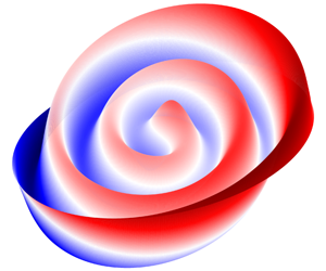
The paper is organised as follows. In § 2, we formulate the sloshing problem and derive a set of modal equations, which is supplemented by linear damping rates. We present explicit solutions for the wave amplitudes and phase shifts which depend on eight independent dimensionless numbers. In § 3, we discuss the resulting wave and resonance dynamics for the different cases considered. As a special feature, the theory predicts the occurrence of novel spiral wave patterns, which are analysed for various damping rates. In § 4, we finally compare theoretical wave amplitudes, phase shifts and fluid velocities with three recently reported experiments. Section 4.3 contains an explanation of the wave elevation’s linear scaling with the Froude number that was found by Weheliye et al. (Reference Weheliye, Yianneskis and Ducci2013) on an empirical basis. Building on this, a prediction for the nonlinear out-of-phase transition is also derived by quantifying the waviness of the free surface.
2 Theory
Analytical solutions to viscous wave dynamics are often difficult if not impossible to find. Therefore, potential flow theory was frequently applied in many early studies to approximate the velocity fields. However, potential flow theory introduces drastic simplifications: the flow is assumed to be inviscid, irrotational and incompressible. Further, wave amplitudes must remain sufficiently low to allow linear or weakly nonlinear approaches. Despite all these restrictions, potential approaches have been quite successful in predicting non-resonant sloshing (Ibrahim Reference Ibrahim2005).

Figure 1. Sketch of the theoretical set-up. A cylinder of radius  $R$ undergoes a harmonic circular translation of diameter $d_{s}$ with a constant angular frequency $\unicode[STIX]{x1D6FA}$. The cylinder contains two fluids $i=1,2$ of densities $\unicode[STIX]{x1D70C}_{i}$, kinematic viscosities $\unicode[STIX]{x1D708}_{i}$ and layer heights $h_{i}$, which are stably stratified due to gravity $\boldsymbol{g}$. The interface with interfacial tension $\unicode[STIX]{x1D6FE}$ is placed at $z=\unicode[STIX]{x1D702}(r,\unicode[STIX]{x1D711},t)$ in the frame of reference moving with the cylinder $O(r,\unicode[STIX]{x1D711},z)$. The inertial frame of reference is indexed by $O^{\prime }(r^{\prime },\unicode[STIX]{x1D711}^{\prime },z^{\prime })$. The orange arrows mark the decompositions of the orbital translation into Cartesian coordinates ( $\boldsymbol{e}_{x}$, $\boldsymbol{e}_{y}$).
Studies tackling viscous wave theories and their higher mathematical complexity are rare. A significant approach for lateral excitation was developed by Bauer & Eidel (Reference Bauer and Eidel1997, Reference Bauer and Eidel1999), who performed a modal analysis starting from the Stokes equations. This approach allows us to calculate responding resonance curves and container forces in direct dependence of the viscosity; however, the solutions are elusive and remain implicit. For this reason, we decided to apply a simpler approach based on potential flow theory. Although potential flow theory can be applied only to irrotational flows, it is possible to include viscous damping rates a posteriori into the modal equations, as described by Faltinsen & Timokha (Reference Faltinsen and Timokha2009, chap. 6). In this way, we neglect the influence of rotational boundary layers on the flow fields and the wave motion, but we can include the energy dissipation resulting from the boundary layers. This approach is valid only if the boundary layers are considerably smaller than the lateral dimensions of the cylinder. The detailed parameter regime fulfilling this condition is discussed in § 2.5.
Very recently, Herreman et al. (Reference Herreman, Nore, Guermond, Cappanera, Weber and Horstmann2019) have derived viscous damping rates for interfacial waves in cylindrical tanks using a perturbative description of Stokes boundary layers. This result finally allows us to derive explicit viscosity-dependent formulas for the resonance curves and phase shifts, which are comparatively easy to handle and simple to apply for further analysis.
2.1 Statement of the problem
Figure 1 shows the set-up for our theoretical framework, analogous to the description given by Reclari (Reference Reclari2013). We define an ideal cylinder of radius  $R$, containing two liquid layers (subscripts $i=1,2$) of heights $h_{1},h_{2}$, kinematic viscosities $\unicode[STIX]{x1D708}_{1},\unicode[STIX]{x1D708}_{2}$ and densities $\unicode[STIX]{x1D70C}_{1},\unicode[STIX]{x1D70C}_{2}$, where $\unicode[STIX]{x1D70C}_{1}<\unicode[STIX]{x1D70C}_{2}$ must be fulfilled to ensure a stable vertical stratification. Gravity $\boldsymbol{g}$ acts in the negative $z$-direction. In cylindrical coordinates ( $r,\unicode[STIX]{x1D711},z$) the interface is located at $z=\unicode[STIX]{x1D702}(r,\unicode[STIX]{x1D711},t)$. Interfacial tension $\unicode[STIX]{x1D6FE}$ is considered along the liquid–liquid interface but capillary forces acting on the contact line are neglected; we assume that the interface may slide freely along the cylinder wall while maintaining a static contact angle of $90^{\circ }$ (no meniscus). The coordinate origin of the moving cylinder, the moving frame of reference $O(r,\unicode[STIX]{x1D711},z)$, is defined in the centre of the unperturbed interface $\unicode[STIX]{x1D702}$. In addition, we define the inertial frame of reference $O^{\prime }(r^{\prime },\unicode[STIX]{x1D711}^{\prime },z^{\prime })$ to describe the circulatory trajectories of the shaking table. The shaker is horizontally translated with a constant angular frequency $\unicode[STIX]{x1D6FA}$ along a circular path $\unicode[STIX]{x1D711}^{\prime }(t)=\unicode[STIX]{x1D6FA}t$ of shaking diameter $d_{s}$.
This formulation is characterised by eleven physical variables and three physical dimensions. Following the Buckingham  $\unicode[STIX]{x03C0}$ theorem, the system can be uniquely described by eight independent dimensionless parameters. We define the following set of dimensionless numbers for our analysis:
 $$\begin{eqnarray}Fr={\displaystyle \frac{d_{s}\unicode[STIX]{x1D6FA}^{2}}{2g}},\quad E={\displaystyle \frac{d_{s}}{2R}},\quad Re_{i}={\displaystyle \frac{\unicode[STIX]{x1D6FA}R^{2}}{\unicode[STIX]{x1D708}_{i}}},\quad H_{i}={\displaystyle \frac{h_{i}}{R}},\quad Bo={\displaystyle \frac{(\unicode[STIX]{x1D70C}_{2}-\unicode[STIX]{x1D70C}_{1})gR^{2}}{\unicode[STIX]{x1D6FE}}},\quad A={\displaystyle \frac{\unicode[STIX]{x1D70C}_{2}-\unicode[STIX]{x1D70C}_{1}}{\unicode[STIX]{x1D70C}_{1}+\unicode[STIX]{x1D70C}_{2}}}.\end{eqnarray}$$
 The Froude number  $Fr$ describes the forcing expressed by the ratio of inertial force and gravitational acceleration. The normalised shaking diameter determines the eccentricity $E$, while $Re_{i}$ are the phase-dependent Reynolds numbers, here weighting the cylinder radius with the boundary layer thicknesses $\unicode[STIX]{x1D6FF}_{i}=\sqrt{\unicode[STIX]{x1D708}_{i}/\unicode[STIX]{x1D6FA}}$. The importance of gravitational forces compared with interfacial tension forces is specified by the Bond number $Bo$. Finally, $H_{i}$ and $A$ are the geometrical aspect ratios and the Atwood number, respectively. It is the aim of our following analysis to relate these numbers to the resulting wave amplitudes and phase shifts.
2.2 Modal equations and solutions
The velocity vector  $\boldsymbol{V}_{0}(t)$ describing the orbital container motion can be expressed in terms of cylindrical unit base vectors in the inertial frame of reference $O^{\prime }(r^{\prime },\unicode[STIX]{x1D711}^{\prime },z^{\prime })$
 $$\begin{eqnarray}\boldsymbol{V}_{0}(t)=\left(\begin{array}{@{}c@{}}-{\displaystyle \frac{d_{s}\unicode[STIX]{x1D6FA}}{2}}\sin (\unicode[STIX]{x1D6FA}t-\unicode[STIX]{x1D711}^{\prime })\boldsymbol{e}_{r^{\prime }}\\[10.0pt] {\displaystyle \frac{d_{s}\unicode[STIX]{x1D6FA}}{2}}\cos (\unicode[STIX]{x1D6FA}t-\unicode[STIX]{x1D711}^{\prime })\boldsymbol{e}_{\unicode[STIX]{x1D711}^{\prime }}\\ \end{array}\right).\end{eqnarray}$$
 Due to this orbital motion the liquids in the cylinder constantly experience rotary acceleration in the moving frame of reference  $O$ resulting in centripetal forces, which can be formulated as external volume forces in the equations of motion for the container-fixed coordinate system. The incompressible Euler equations for $O$ under the influence of gravity $\boldsymbol{g}$ and subject to $\boldsymbol{V}_{0}$ are
 $$\begin{eqnarray}\displaystyle & \displaystyle {\displaystyle \frac{\unicode[STIX]{x2202}\boldsymbol{u}_{i}}{\unicode[STIX]{x2202}t}}+{\displaystyle \frac{1}{2}}\unicode[STIX]{x1D735}|\boldsymbol{u}_{i}^{2}|-\boldsymbol{u}_{i}\times (\unicode[STIX]{x1D735}\times \boldsymbol{u}_{i})+{\displaystyle \frac{1}{\unicode[STIX]{x1D70C}_{i}}}\unicode[STIX]{x1D735}P_{i}-\boldsymbol{g}+\dot{\boldsymbol{V}}_{0}=0, & \displaystyle\end{eqnarray}$$
 $$\begin{eqnarray}\displaystyle & \displaystyle \unicode[STIX]{x1D735}\boldsymbol{\cdot }\boldsymbol{u}_{i}=0, & \displaystyle\end{eqnarray}$$
 (compare with Kochin, Kibel & Roze (Reference Kochin, Kibel and Roze1964, chap. 2)), where  $\boldsymbol{u}_{i}$ are the relative velocity fields and $P_{i}$ the pressures associated with both fluids $(i=1,2)$. By postulating irrotationality ( $\unicode[STIX]{x1D735}\times \boldsymbol{u}_{i}=0$), the potential flow approximation can be applied stating that the flow fields $\boldsymbol{u}_{i}$ can be uniquely expressed as gradients of scalar potentials $\unicode[STIX]{x1D719}_{i}$
 $$\begin{eqnarray}\boldsymbol{u}_{i}=\unicode[STIX]{x1D735}\unicode[STIX]{x1D719}_{i}.\end{eqnarray}$$
 By inserting (2.5) into (2.3) and (2.4) and integrating over the cylinder volume, a complete set of governing equations and boundary conditions for the scalar flow potentials  $\unicode[STIX]{x1D719}_{i}$, the pressures $P_{i}$ and the interface position $\unicode[STIX]{x1D702}$ can be formulated
 $$\begin{eqnarray}\displaystyle \text{Flow fields:}\!\quad & & \displaystyle {\displaystyle \frac{\unicode[STIX]{x2202}\unicode[STIX]{x1D719}_{i}}{\unicode[STIX]{x2202}t}}-{\displaystyle \frac{d_{s}\unicode[STIX]{x1D6FA}^{2}r}{2}}\cos (\unicode[STIX]{x1D6FA}t-\unicode[STIX]{x1D711})+{\displaystyle \frac{1}{2}}(\unicode[STIX]{x1D735}\unicode[STIX]{x1D719}_{i})^{2}+{\displaystyle \frac{P_{i}}{\unicode[STIX]{x1D70C}_{i}}}+gz=c_{i}(t),\end{eqnarray}$$
 $$\begin{eqnarray}\displaystyle \displaystyle \text{Flow fields:}\!\quad & & \displaystyle \unicode[STIX]{x0394}\unicode[STIX]{x1D719}_{i}=0,\end{eqnarray}$$
 $$\begin{eqnarray}\displaystyle \displaystyle \text{Top wall:}\!\quad & & \displaystyle {\displaystyle \frac{\unicode[STIX]{x2202}\unicode[STIX]{x1D719}_{1}}{\unicode[STIX]{x2202}z}}=0|_{z=h_{1}},\end{eqnarray}$$
 $$\begin{eqnarray}\displaystyle \displaystyle \text{Bottom wall:}\!\quad & & \displaystyle {\displaystyle \frac{\unicode[STIX]{x2202}\unicode[STIX]{x1D719}_{2}}{\unicode[STIX]{x2202}z}}=0|_{z=-h_{2}},\end{eqnarray}$$
 $$\begin{eqnarray}\displaystyle \displaystyle \text{Sidewall:}\!\quad & & \displaystyle {\displaystyle \frac{\unicode[STIX]{x2202}\unicode[STIX]{x1D719}_{1}}{\unicode[STIX]{x2202}r}}={\displaystyle \frac{\unicode[STIX]{x2202}\unicode[STIX]{x1D719}_{2}}{\unicode[STIX]{x2202}r}}=0|_{r=R},\end{eqnarray}$$
 $$\begin{eqnarray}\displaystyle \displaystyle \text{Interface:}\!\quad & & \displaystyle {\displaystyle \frac{\unicode[STIX]{x2202}\unicode[STIX]{x1D719}_{1}}{\unicode[STIX]{x2202}z}}={\displaystyle \frac{\unicode[STIX]{x2202}\unicode[STIX]{x1D719}_{2}}{\unicode[STIX]{x2202}z}}={\displaystyle \frac{\unicode[STIX]{x2202}\unicode[STIX]{x1D702}}{\unicode[STIX]{x2202}t}}+\unicode[STIX]{x1D735}\unicode[STIX]{x1D719}_{i}\boldsymbol{\cdot }\unicode[STIX]{x1D735}\unicode[STIX]{x1D702}|_{z=\unicode[STIX]{x1D702}},\end{eqnarray}$$
 $$\begin{eqnarray}\displaystyle \displaystyle \text{Interface:}\!\quad & & \displaystyle \unicode[STIX]{x1D6FE}\unicode[STIX]{x1D735}\boldsymbol{\cdot }{\displaystyle \frac{\unicode[STIX]{x1D735}\unicode[STIX]{x1D702}}{\sqrt{1+|\unicode[STIX]{x1D735}\unicode[STIX]{x1D702}|^{2}}}}=P_{1}-P_{2}|_{z=\unicode[STIX]{x1D702}}.\end{eqnarray}$$
 This formulation represents a class of spectral sloshing problems well known in the literature. Faltinsen & Timokha (Reference Faltinsen and Timokha2009) introduce different modal theories to find approximate analytical solutions for free-surface sloshing problems, mathematically quite similar to our two-layer formulation. In this study, we want to focus on first-order linear solutions, which are reasonable approximations as long as the wave amplitudes remain sufficiently small. In the linear approximation, the flow potentials  $\unicode[STIX]{x1D719}_{i}$ can be described as superpositions of an infinite number of independent sloshing modes $m\in \mathbb{N}_{0}$ and $n\in \mathbb{N}_{1}$
 $$\begin{eqnarray}\displaystyle & & \displaystyle \unicode[STIX]{x1D719}_{1}(r,\unicode[STIX]{x1D711},z,t)=-\mathop{\sum }_{m=0}^{\infty }\mathop{\sum }_{n=1}^{\infty }\unicode[STIX]{x1D6F7}_{mn}(\unicode[STIX]{x1D711},t){\displaystyle \frac{\cosh \left({\displaystyle \frac{\unicode[STIX]{x1D716}_{mn}}{R}}(z-h_{1})\right)}{\sinh \left({\displaystyle \frac{\unicode[STIX]{x1D716}_{mn}}{R}}h_{1}\right)}}J_{m}\left(\unicode[STIX]{x1D716}_{mn}\frac{r}{R}\right),\end{eqnarray}$$
 $$\begin{eqnarray}\displaystyle & & \displaystyle \unicode[STIX]{x1D719}_{2}(r,\unicode[STIX]{x1D711},z,t)=\mathop{\sum }_{m=0}^{\infty }\mathop{\sum }_{n=1}^{\infty }\unicode[STIX]{x1D6F7}_{mn}(\unicode[STIX]{x1D711},t){\displaystyle \frac{\cosh \left({\displaystyle \frac{\unicode[STIX]{x1D716}_{mn}}{R}}(z+h_{2})\right)}{\sinh \left({\displaystyle \frac{\unicode[STIX]{x1D716}_{mn}}{R}}h_{2}\right)}}J_{m}\left(\unicode[STIX]{x1D716}_{mn}{\displaystyle \frac{r}{R}}\right),\end{eqnarray}$$
 $$\begin{eqnarray}\displaystyle & & \displaystyle \quad \text{with }\unicode[STIX]{x1D6F7}_{mn}(\unicode[STIX]{x1D711},t)=\unicode[STIX]{x1D6FC}_{mn}(t)\cos (m\unicode[STIX]{x1D711})+\unicode[STIX]{x1D6FD}_{mn}(t)\sin (m\unicode[STIX]{x1D711}),\end{eqnarray}$$ $\unicode[STIX]{x1D6FC}_{mn}(t)$ and $\unicode[STIX]{x1D6FD}_{mn}(t)$ are the time-dependent modal functions to be determined, $J_{m}$ are the $m$th-order Bessel functions of the first kind and $\unicode[STIX]{x1D716}_{mn}$ denote the mode-dependent wavenumbers, restricted to the $n$ roots of the first derivative of the $m$th-order Bessel function ( $J_{m}^{^{\prime }}(\unicode[STIX]{x1D716}_{mn})=0$; Abramowitz & Stegun (Reference Abramowitz and Stegun1972)), needed to satisfy the no-outflow condition at the sidewalls; $\unicode[STIX]{x1D716}_{mn}$ are often called the radial wavenumbers since they determine the number of crests in the radial direction. Accordingly, $m$ denote the azimuthal wavenumbers.
 In order for the flow potentials (2.7) to fulfil (2.6), we have to specify the modal functions  $\unicode[STIX]{x1D6FC}_{mn}(t)$ and $\unicode[STIX]{x1D6FD}_{mn}(t)$. Linear model theories show that the modal functions always obey a multidimensional system of ordinary differential equations. Faltinsen & Timokha (Reference Faltinsen and Timokha2009, equation (5.155)) have derived the modal equations in the case of one fluid layer, which are mathematically very similar to our interfacial sloshing problem. By following their procedures, we find the modal equations
 $$\begin{eqnarray}\displaystyle & \displaystyle \ddot{\unicode[STIX]{x1D6FC}}_{1n}(t)+2\unicode[STIX]{x1D706}_{1n}\dot{\unicode[STIX]{x1D6FC}}_{1n}(t)+\unicode[STIX]{x1D714}_{1n}^{2}\unicode[STIX]{x1D6FC}_{1n}(t)-\unicode[STIX]{x1D701}_{n}\sin (\unicode[STIX]{x1D6FA}t)=0, & \displaystyle\end{eqnarray}$$
 $$\begin{eqnarray}\displaystyle & \displaystyle \ddot{\unicode[STIX]{x1D6FD}}_{1n}(t)+2\unicode[STIX]{x1D706}_{1n}\dot{\unicode[STIX]{x1D6FD}}_{1n}(t)+\unicode[STIX]{x1D714}_{1n}^{2}\unicode[STIX]{x1D6FD}_{1n}(t)+\unicode[STIX]{x1D701}_{n}\cos (\unicode[STIX]{x1D6FA}t)=0, & \displaystyle\end{eqnarray}$$
 $$\begin{eqnarray}\displaystyle & \displaystyle \unicode[STIX]{x1D714}_{1n}^{2}={\displaystyle \frac{(\unicode[STIX]{x1D70C}_{2}-\unicode[STIX]{x1D70C}_{1})g{\displaystyle \frac{\unicode[STIX]{x1D716}_{1n}}{R}}+\unicode[STIX]{x1D6FE}\left({\displaystyle \frac{\unicode[STIX]{x1D716}_{1n}}{R}}\right)^{3}}{\unicode[STIX]{x1D70C}_{1}\coth \left({\displaystyle \frac{\unicode[STIX]{x1D716}_{1n}}{R}}h_{1}\right)+\unicode[STIX]{x1D70C}_{2}\coth \left({\displaystyle \frac{\unicode[STIX]{x1D716}_{1n}}{R}}h_{2}\right)}}, & \displaystyle\end{eqnarray}$$
 $$\begin{eqnarray}\displaystyle & \displaystyle \unicode[STIX]{x1D701}_{n}={\displaystyle \frac{(\unicode[STIX]{x1D70C}_{2}-\unicode[STIX]{x1D70C}_{1})Rd_{s}\unicode[STIX]{x1D6FA}^{3}}{\left(\unicode[STIX]{x1D70C}_{1}\coth \left({\displaystyle \frac{\unicode[STIX]{x1D716}_{1n}}{R}}h_{1}\right)+\unicode[STIX]{x1D70C}_{2}\coth \left({\displaystyle \frac{\unicode[STIX]{x1D716}_{1n}}{R}}h_{2}\right)\right)(\unicode[STIX]{x1D716}_{1n}^{2}-1)J_{1}(\unicode[STIX]{x1D716}_{1n})}}, & \displaystyle\end{eqnarray}$$
 to be fulfilled for  $\unicode[STIX]{x1D6FC}_{mn}(t)$ and $\unicode[STIX]{x1D6FD}_{mn}(t)$, where we have included linear damping rates $\unicode[STIX]{x1D706}_{1n}$ expressing the energy dissipation as explained by Faltinsen & Timokha (Reference Faltinsen and Timokha2009, chap. 6). Here, $\unicode[STIX]{x1D714}_{1n}^{2}$ are the natural eigenfrequencies of two-layer gravity–capillary waves in cylindrical tanks, while $\unicode[STIX]{x1D701}_{n}$ can be understood as a mode-dependent forcing parameter describing the strength of excitation. Please note that only non-axisymmetric wave modes $(m=1)$ are excited in the linear regime, possessing exactly one nodal circle. Linear solutions do not exist for $m\neq 1$.
Equations (2.8a) and (2.8b) have the following stationary solutions:
 $$\begin{eqnarray}\displaystyle \hspace{-12.0pt}\unicode[STIX]{x1D6FC}_{1n}(t) & = & \displaystyle {\displaystyle \frac{\unicode[STIX]{x1D701}_{n}(\unicode[STIX]{x1D714}_{1n}^{2}-\unicode[STIX]{x1D6FA}^{2})}{(\unicode[STIX]{x1D714}_{1n}^{2}-\unicode[STIX]{x1D6FA}^{2})^{2}+4\unicode[STIX]{x1D706}_{1n}^{2}\unicode[STIX]{x1D6FA}^{2}}}\sin (\unicode[STIX]{x1D6FA}t)-{\displaystyle \frac{2\unicode[STIX]{x1D706}_{1n}\unicode[STIX]{x1D701}_{n}\unicode[STIX]{x1D6FA}}{(\unicode[STIX]{x1D714}_{1n}^{2}-\unicode[STIX]{x1D6FA}^{2})^{2}+4\unicode[STIX]{x1D706}_{1n}^{2}\unicode[STIX]{x1D6FA}^{2}}}\cos (\unicode[STIX]{x1D6FA}t),\qquad\end{eqnarray}$$
 $$\begin{eqnarray}\displaystyle \hspace{-12.0pt}\unicode[STIX]{x1D6FD}_{1n}(t) & = & \displaystyle -{\displaystyle \frac{\unicode[STIX]{x1D701}_{n}(\unicode[STIX]{x1D714}_{1n}^{2}-\unicode[STIX]{x1D6FA}^{2})}{(\unicode[STIX]{x1D714}_{1n}^{2}-\unicode[STIX]{x1D6FA}^{2})^{2}+4\unicode[STIX]{x1D706}_{1n}^{2}\unicode[STIX]{x1D6FA}^{2}}}\cos (\unicode[STIX]{x1D6FA}t)-{\displaystyle \frac{2\unicode[STIX]{x1D706}_{1n}\unicode[STIX]{x1D701}_{n}\unicode[STIX]{x1D6FA}}{(\unicode[STIX]{x1D714}_{1n}^{2}-\unicode[STIX]{x1D6FA}^{2})^{2}+4\unicode[STIX]{x1D706}_{1n}^{2}\unicode[STIX]{x1D6FA}^{2}}}\sin (\unicode[STIX]{x1D6FA}t).\qquad\end{eqnarray}$$
 $$\begin{eqnarray}\displaystyle & & \displaystyle \hspace{-9.60004pt}\unicode[STIX]{x1D719}_{1}(r,\unicode[STIX]{x1D711},z,t)=\mathop{\sum }_{n=1}^{\infty }{\displaystyle \frac{(\unicode[STIX]{x1D70C}_{2}-\unicode[STIX]{x1D70C}_{1})Rd_{s}\unicode[STIX]{x1D6FA}^{3}}{\left(\unicode[STIX]{x1D70C}_{1}\coth \left({\displaystyle \frac{\unicode[STIX]{x1D716}_{1n}}{R}}h_{1}\right)+\unicode[STIX]{x1D70C}_{2}\coth \left({\displaystyle \frac{\unicode[STIX]{x1D716}_{1n}}{R}}h_{2}\right)\right)}}{\displaystyle \frac{\cosh \left({\displaystyle \frac{\unicode[STIX]{x1D716}_{1n}}{R}}(z-h_{1})\right)}{\sinh \left({\displaystyle \frac{\unicode[STIX]{x1D716}_{1n}}{R}}h_{1}\right)}}{\displaystyle \frac{J_{1}\left(\unicode[STIX]{x1D716}_{1n}{\displaystyle \frac{r}{R}}\right)}{(\unicode[STIX]{x1D716}_{1n}^{2}-1)J_{1}(\unicode[STIX]{x1D716}_{1n})}}\nonumber\\ \displaystyle & & \displaystyle \hspace{-9.60004pt}\quad \times \left[{\displaystyle \frac{(\unicode[STIX]{x1D714}_{1n}^{2}-\unicode[STIX]{x1D6FA}^{2})}{(\unicode[STIX]{x1D714}_{1n}^{2}-\unicode[STIX]{x1D6FA}^{2})^{2}+4\unicode[STIX]{x1D706}_{1n}^{2}\unicode[STIX]{x1D6FA}^{2}}}\sin (\unicode[STIX]{x1D6FA}t-\unicode[STIX]{x1D711})-{\displaystyle \frac{2\unicode[STIX]{x1D706}_{1n}\unicode[STIX]{x1D6FA}}{(\unicode[STIX]{x1D714}_{1n}^{2}-\unicode[STIX]{x1D6FA}^{2})^{2}+4\unicode[STIX]{x1D706}_{1n}^{2}\unicode[STIX]{x1D6FA}^{2}}}\cos (\unicode[STIX]{x1D6FA}t-\unicode[STIX]{x1D711})\right]\!,\end{eqnarray}$$
 $$\begin{eqnarray}\displaystyle & & \displaystyle \hspace{-9.60004pt}\unicode[STIX]{x1D719}_{2}(r,\unicode[STIX]{x1D711},z,t)=\mathop{\sum }_{n=1}^{\infty }{\displaystyle \frac{-(\unicode[STIX]{x1D70C}_{2}-\unicode[STIX]{x1D70C}_{1})Rd_{s}\unicode[STIX]{x1D6FA}^{3}}{\left(\unicode[STIX]{x1D70C}_{1}\coth \left({\displaystyle \frac{\unicode[STIX]{x1D716}_{1n}}{R}}h_{1}\right)+\unicode[STIX]{x1D70C}_{2}\coth \left({\displaystyle \frac{\unicode[STIX]{x1D716}_{1n}}{R}}h_{2}\right)\right)}}{\displaystyle \frac{\cosh \left({\displaystyle \frac{\unicode[STIX]{x1D716}_{1n}}{R}}(z+h_{2})\right)}{\sinh \left({\displaystyle \frac{\unicode[STIX]{x1D716}_{1n}}{R}}h_{2}\right)}}{\displaystyle \frac{J_{1}\left(\unicode[STIX]{x1D716}_{1n}{\displaystyle \frac{r}{R}}\right)}{(\unicode[STIX]{x1D716}_{1n}^{2}-1)J_{1}(\unicode[STIX]{x1D716}_{1n})}}\nonumber\\ \displaystyle & & \displaystyle \hspace{-9.60004pt}\quad \times \left[{\displaystyle \frac{(\unicode[STIX]{x1D714}_{1n}^{2}-\unicode[STIX]{x1D6FA}^{2})}{(\unicode[STIX]{x1D714}_{1n}^{2}-\unicode[STIX]{x1D6FA}^{2})^{2}+4\unicode[STIX]{x1D706}_{1n}^{2}\unicode[STIX]{x1D6FA}^{2}}}\sin (\unicode[STIX]{x1D6FA}t-\unicode[STIX]{x1D711})-{\displaystyle \frac{2\unicode[STIX]{x1D706}_{1n}\unicode[STIX]{x1D6FA}}{(\unicode[STIX]{x1D714}_{1n}^{2}-\unicode[STIX]{x1D6FA}^{2})^{2}+4\unicode[STIX]{x1D706}_{1n}^{2}\unicode[STIX]{x1D6FA}^{2}}}\cos (\unicode[STIX]{x1D6FA}t-\unicode[STIX]{x1D711})\right]\!.\end{eqnarray}$$ $\unicode[STIX]{x1D702}$ is determined by linearising (2.6f). It can be expressed as
  $$\begin{eqnarray}\displaystyle & & \displaystyle \hspace{-36.0pt}\unicode[STIX]{x1D702}(r,\unicode[STIX]{x1D711},t)=\mathop{\sum }_{n=1}^{\infty }{\displaystyle \frac{(\unicode[STIX]{x1D70C}_{2}-\unicode[STIX]{x1D70C}_{1})d_{s}R\unicode[STIX]{x1D6FA}^{2}}{\left[(\unicode[STIX]{x1D70C}_{2}-\unicode[STIX]{x1D70C}_{1})g+\left({\displaystyle \frac{\unicode[STIX]{x1D716}_{1n}}{R}}\right)^{2}\unicode[STIX]{x1D6FE}\right]}}{\displaystyle \frac{J_{1}\left(\unicode[STIX]{x1D716}_{1n}{\displaystyle \frac{r}{R}}\right)}{(\unicode[STIX]{x1D716}_{1n}^{2}-1)J_{1}(\unicode[STIX]{x1D716}_{1n})}}\nonumber\\ \displaystyle & & \displaystyle \hspace{-42.0pt}\quad \times \left[{\displaystyle \frac{\unicode[STIX]{x1D714}_{1n}^{2}(\unicode[STIX]{x1D714}_{1n}^{2}-\unicode[STIX]{x1D6FA}^{2})}{(\unicode[STIX]{x1D714}_{1n}^{2}-\unicode[STIX]{x1D6FA}^{2})^{2}+4\unicode[STIX]{x1D706}_{1n}^{2}\unicode[STIX]{x1D6FA}^{2}}}\cos (\unicode[STIX]{x1D6FA}t-\unicode[STIX]{x1D711})+{\displaystyle \frac{2\unicode[STIX]{x1D706}_{1n}\unicode[STIX]{x1D6FA}\unicode[STIX]{x1D714}_{1n}^{2}}{(\unicode[STIX]{x1D714}_{1n}^{2}-\unicode[STIX]{x1D6FA}^{2})^{2}+4\unicode[STIX]{x1D706}_{1n}^{2}\unicode[STIX]{x1D6FA}^{2}}}\sin (\unicode[STIX]{x1D6FA}t-\unicode[STIX]{x1D711})\!\right]\!.\end{eqnarray}$$
 As a main difference from the previous inviscid theories, the azimuthal part of our solution is composed of both a symmetric  ${\sim}\cos (\unicode[STIX]{x1D6FA}t-\unicode[STIX]{x1D711})$ and an antisymmetric ${\sim}\sin (\unicode[STIX]{x1D6FA}t-\unicode[STIX]{x1D711})$ contribution, whereas inviscid solutions are always symmetric. In the limit $\unicode[STIX]{x1D70C}_{2},\unicode[STIX]{x1D706}_{1n},\unicode[STIX]{x1D6FE}\mapsto 0$ this solution is equivalent to the inviscid one-layer theory by Reclari et al. (Reference Reclari, Dreyer, Tissot, Obreschkow, Wurm and Farhat2014), as we prove in appendix B. From (2.13) we can deduce the resonance frequencies $\unicode[STIX]{x1D714}_{R,n}$ of the wave modes which are modified by damping. Close to resonance ( $\unicode[STIX]{x1D6FA}\approx \unicode[STIX]{x1D714}_{1n}$) the interface elevation is described only by the antisymmetric part of the solution. Therefore
 $$\begin{eqnarray}\unicode[STIX]{x1D702}(r,\unicode[STIX]{x1D711}=\unicode[STIX]{x1D6FA}t-\unicode[STIX]{x03C0}/2,t)|_{\unicode[STIX]{x1D6FA}\approx \unicode[STIX]{x1D714}_{1n}}=A{\displaystyle \frac{2\unicode[STIX]{x1D706}_{1n}\unicode[STIX]{x1D6FA}^{3}\unicode[STIX]{x1D714}_{1n}^{2}}{(\unicode[STIX]{x1D714}_{1n}^{2}-\unicode[STIX]{x1D6FA}^{2})^{2}+4\unicode[STIX]{x1D706}_{1n}^{2}\unicode[STIX]{x1D6FA}^{2}}},\end{eqnarray}$$
 where  $A$ contains the frequency-independent prefactors of (2.13). The shaking frequency causing the highest amplitude ( $\unicode[STIX]{x1D6FA}\equiv \unicode[STIX]{x1D714}_{R,n}$) is calculated by solving
 $$\begin{eqnarray}{\displaystyle \frac{\unicode[STIX]{x2202}\unicode[STIX]{x1D702}(r,\unicode[STIX]{x1D711}=\unicode[STIX]{x1D6FA}t-\unicode[STIX]{x03C0}/2,t)}{\unicode[STIX]{x2202}\unicode[STIX]{x1D6FA}}}=0\end{eqnarray}$$
giving a resonance frequency of
 $$\begin{eqnarray}\unicode[STIX]{x1D714}_{R,n}^{2}=2\sqrt{(\unicode[STIX]{x1D714}_{1n}^{2}-\unicode[STIX]{x1D706}_{1n}^{2})^{2}+\unicode[STIX]{x1D706}_{1n}^{2}\unicode[STIX]{x1D714}_{1n}^{2}}-\unicode[STIX]{x1D714}_{1n}^{2}+2\unicode[STIX]{x1D706}_{1n}^{2}\geqslant \unicode[STIX]{x1D714}_{1n}^{2}.\end{eqnarray}$$
 Thus, high damping rates always increase the resonance frequency. This behaviour might appear counterintuitive and is contrary to that of the classical driven harmonic oscillator. It is caused by differences of the external forcing. The forcing amplitude itself depends on the driving frequency and scales with  ${\sim}\unicode[STIX]{x1D6FA}^{3}$ (see (2.10)), introducing the tendency that the wave is generally amplified for higher shaking frequencies independently of the resonant amplifications. This effect overcompensates the common frequency drop observed in systems underlying a constant driving force ( $\unicode[STIX]{x1D701}_{n}$ independent of $\unicode[STIX]{x1D6FA}$). However, in practical applications, as with OSBs, a noticeable increase of the eigenfrequency will not be observable for the first modes due to their weak dependency on $\unicode[STIX]{x1D706}_{1n}$ in (2.16) for common damping rates $\unicode[STIX]{x1D706}_{1n}\lesssim 1$. An increase of $\unicode[STIX]{x1D714}_{R,n}$ would be observable only in highly overdamped set-ups. For weakly damped systems we identify $\unicode[STIX]{x1D714}_{R,n}\approx \unicode[STIX]{x1D714}_{1n}$ (at least for the first important large-scale wave modes).
2.3 Viscous damping
Equation (2.13) is the final result of the modal analysis containing the responding resonance dynamics of the interface. In contrast to previous inviscid theories (Reclari et al. Reference Reclari, Dreyer, Tissot, Obreschkow, Wurm and Farhat2014; Bouvard et al. Reference Bouvard, Herreman and Moisy2017), our solution does not contain any singularities at the resonance frequencies. Those are resolved by the damping parameters  $\unicode[STIX]{x1D706}_{1n}$ determining the maximum amplitudes at resonance $\unicode[STIX]{x1D6FA}\approx \unicode[STIX]{x1D714}_{1n}$. However, using an irrotational approach, the damping rates cannot be further deduced since viscous dissipation is caused by the rotational part of the flow manifested in the boundary layers. Therefore, damping rates must be determined a priori, i.e. by fitting the exponential decay of resonant waves after the shaker is switched off. Then, equation (2.13) can predict the wave amplitudes (within its limits) for all shaking frequencies $\unicode[STIX]{x1D6FA}$ around the considered resonance frequency.
However, to allow for further analysis and a better understanding of how viscous damping can affect the resonance dynamics, it is desirable to describe the wave elevation in direct dependence of the viscosities  $\unicode[STIX]{x1D708}_{i}$. For that purpose, we exploit some of the recent results given by Herreman et al. (Reference Herreman, Nore, Guermond, Cappanera, Weber and Horstmann2019), who applied a perturbation approach to study interfacial wave damping. They derived viscous damping rates of free gravity–capillary waves by explicitly calculating Stokes boundary layers for the same two-layer geometry that we are considering in the present paper. It was found in this study that viscous damping rates of free-surface and interfacial waves are inherently different, so that we must carefully distinguish between the one- and two-layer limit of viscous damping rates in the following.
In the first order, the two-layer damping rate  $\unicode[STIX]{x1D706}_{1n}^{2L}$ is composed of three different contributions
 $$\begin{eqnarray}\displaystyle \unicode[STIX]{x1D706}_{1n}^{2L}=\unicode[STIX]{x1D706}_{1n}^{BL}+\unicode[STIX]{x1D706}_{1n}^{IL}+\unicode[STIX]{x1D706}_{1n}^{Int},\end{eqnarray}$$
with
 $$\begin{eqnarray}\displaystyle \unicode[STIX]{x1D706}_{1n}^{BL} & = & \displaystyle \mathop{\sum }_{i=1,2}\unicode[STIX]{x1D70C}_{i}\sqrt{{\displaystyle \frac{\unicode[STIX]{x1D708}_{i}\unicode[STIX]{x1D6FA}}{8R^{2}}}}\!\left[{\displaystyle \frac{\unicode[STIX]{x1D716}_{1n}\!\left(1-{\displaystyle \frac{h_{i}}{R}}\right)\sinh ^{-2}\left({\displaystyle \frac{\unicode[STIX]{x1D716}_{1n}}{R}}h_{i}\right)+\left({\displaystyle \frac{\unicode[STIX]{x1D716}_{1n}^{2}+1}{\unicode[STIX]{x1D716}_{1n}^{2}-1}}\right)\coth \left({\displaystyle \frac{\unicode[STIX]{x1D716}_{1n}}{R}}h_{i}\right)}{\unicode[STIX]{x1D70C}_{1}\coth \left({\displaystyle \frac{\unicode[STIX]{x1D716}_{1n}}{R}}h_{1}\right)+\unicode[STIX]{x1D70C}_{2}\coth \left({\displaystyle \frac{\unicode[STIX]{x1D716}_{1n}}{R}}h_{2}\right)}}\!\right]\!\!,\qquad\end{eqnarray}$$
 $$\begin{eqnarray}\displaystyle \unicode[STIX]{x1D706}_{1n}^{IL} & = & \displaystyle {\displaystyle \frac{\unicode[STIX]{x1D716}_{1n}}{\left({\displaystyle \frac{1}{\unicode[STIX]{x1D70C}_{1}}}\sqrt{{\displaystyle \frac{8R^{2}}{\unicode[STIX]{x1D6FA}\unicode[STIX]{x1D708}_{1}}}}+{\displaystyle \frac{1}{\unicode[STIX]{x1D70C}_{2}}}\sqrt{{\displaystyle \frac{8R^{2}}{\unicode[STIX]{x1D6FA}\unicode[STIX]{x1D708}_{2}}}}\right)}}\left[{\displaystyle \frac{\left(\coth \left({\displaystyle \frac{\unicode[STIX]{x1D716}_{1n}}{R}}h_{1}\right)+\coth \left({\displaystyle \frac{\unicode[STIX]{x1D716}_{1n}}{R}}h_{2}\right)\right)^{2}}{\unicode[STIX]{x1D70C}_{1}\coth \left({\displaystyle \frac{\unicode[STIX]{x1D716}_{1n}}{R}}h_{1}\right)+\unicode[STIX]{x1D70C}_{2}\coth \left({\displaystyle \frac{\unicode[STIX]{x1D716}_{1n}}{R}}h_{2}\right)}}\right]\!,\end{eqnarray}$$
 $$\begin{eqnarray}\displaystyle \unicode[STIX]{x1D706}_{1n}^{Int} & = & \displaystyle {\displaystyle \frac{2\unicode[STIX]{x1D716}_{1n}^{2}\left({\displaystyle \frac{\unicode[STIX]{x1D70C}_{2}\unicode[STIX]{x1D708}_{2}}{R^{2}}}-{\displaystyle \frac{\unicode[STIX]{x1D70C}_{1}\unicode[STIX]{x1D708}_{1}}{R^{2}}}\right)}{\left({\displaystyle \frac{1}{\unicode[STIX]{x1D70C}_{1}\sqrt{\unicode[STIX]{x1D708}_{1}}}}+{\displaystyle \frac{1}{\unicode[STIX]{x1D70C}_{2}\sqrt{\unicode[STIX]{x1D708}_{2}}}}\right)}}\left[{\displaystyle \frac{{\displaystyle \frac{1}{\unicode[STIX]{x1D70C}_{1}\sqrt{\unicode[STIX]{x1D708}_{1}}}}\coth \left({\displaystyle \frac{\unicode[STIX]{x1D716}_{1n}}{R}}h_{2}\right)-{\displaystyle \frac{1}{\unicode[STIX]{x1D70C}_{2}\sqrt{\unicode[STIX]{x1D708}_{2}}}}\coth \left({\displaystyle \frac{\unicode[STIX]{x1D716}_{1n}}{R}}h_{1}\right)}{\left(\unicode[STIX]{x1D70C}_{1}\coth \left({\displaystyle \frac{\unicode[STIX]{x1D716}_{1n}}{R}}h_{1}\right)+\unicode[STIX]{x1D70C}_{2}\coth \left({\displaystyle \frac{\unicode[STIX]{x1D716}_{1n}}{R}}h_{2}\right)\right)}}\right]\!.\qquad\end{eqnarray}$$
 The first contribution  $\unicode[STIX]{x1D706}_{1n}^{BL}$ involves viscous dissipation arising at the solid tank boundary layers including the side, top and bottom walls. The second term $\unicode[STIX]{x1D706}_{1n}^{IL}$ describes the dissipation rate in the interfacial boundary layers above and below the interface. Finally, $\unicode[STIX]{x1D706}_{1n}^{Int}$ is the interior damping rate which can be destabilising. Please note that this damping rate is fundamentally different from the well-known damping rates of free-surface waves in upright cylinders calculated by Case & Parkinson (Reference Case and Parkinson1956) and Miles & Henderson (Reference Miles and Henderson1998). The first solid boundary layer term $\unicode[STIX]{x1D706}_{1n}^{BL}$ is physically the same as for one-layer systems. The one-layer limit $\unicode[STIX]{x1D70C}_{1}\mapsto 0$ of $\unicode[STIX]{x1D706}_{1n}^{BL}$ is equivalent to the boundary layer term derived by Case & Parkinson (Reference Case and Parkinson1956). However, the interfacial layer contribution $\unicode[STIX]{x1D706}_{1n}^{IL}$ does not exist in free-surface waves in the leading order. The reason is that the flow field under free surfaces is to a good approximation irrotational, which is not the case around moving interfaces, where viscous boundary layers evolve to balance the strong tangential shear flows between the liquids. Indeed, we find $\unicode[STIX]{x1D706}_{1n}^{IL}\mapsto 0$ for $\unicode[STIX]{x1D70C}_{1}\mapsto 0$. For liquids with similar densities and viscosities $\unicode[STIX]{x1D706}_{1n}^{BL}$ and $\unicode[STIX]{x1D706}_{1n}^{IL}$ can have comparable magnitudes and should always both be considered. In contrast, the interior damping rate $\unicode[STIX]{x1D706}_{1n}^{Int}$ is completely negligible for liquids with densities of the same order. However, this term cannot be ignored anymore when we approach the free-surface limit $\unicode[STIX]{x1D70C}_{1}\mapsto 0$. Then, the interior damping is increased by orders of magnitude until it reaches the limit $\unicode[STIX]{x1D706}_{1n}^{Int}\mapsto 2\unicode[STIX]{x1D708}_{2}\unicode[STIX]{x1D716}_{1n}^{2}/R^{2}$, the familiar interior damping rate of free-surface waves that is generally not negligible. This is the only remaining dissipation term for irrotational surface waves, while interfacial wave damping is always manifested in rotational boundary layers. All in all, leading-order interfacial damping is well described by
 $$\begin{eqnarray}\unicode[STIX]{x1D706}_{1n}^{2L}=\unicode[STIX]{x1D706}_{1n}^{BL}+\unicode[STIX]{x1D706}_{1n}^{IL}.\end{eqnarray}$$
In contrast, free-surface damping must be calculated using the contributions
 $$\begin{eqnarray}\unicode[STIX]{x1D706}_{1n}^{1L}=\unicode[STIX]{x1D706}_{1n}^{BL}+\tilde{\unicode[STIX]{x1D706}}_{1n}^{Int},\end{eqnarray}$$
with
 $$\begin{eqnarray}\displaystyle & \displaystyle \unicode[STIX]{x1D706}_{1n}^{BL}=\sqrt{{\displaystyle \frac{\unicode[STIX]{x1D708}_{2}\unicode[STIX]{x1D6FA}}{8R^{2}}}}\left[{\displaystyle \frac{\unicode[STIX]{x1D716}_{1n}^{2}+1}{\unicode[STIX]{x1D716}_{1n}^{2}-1}}+{\displaystyle \frac{2\unicode[STIX]{x1D716}_{1n}\left(1-{\displaystyle \frac{h_{2}}{R}}\right)}{\sinh \left(2{\displaystyle \frac{\unicode[STIX]{x1D716}_{1n}}{R}}h_{2}\right)}}\right]\!, & \displaystyle\end{eqnarray}$$
 $$\begin{eqnarray}\displaystyle & \displaystyle \tilde{\unicode[STIX]{x1D706}}_{1n}^{Int}={\displaystyle \frac{\unicode[STIX]{x1D708}_{2}}{R^{2}}}\left[2\unicode[STIX]{x1D716}_{1n}^{2}-{\displaystyle \frac{1}{\unicode[STIX]{x1D716}_{1n}^{2}-1}}\left(1+{\displaystyle \frac{2\unicode[STIX]{x1D716}_{1n}h_{2}}{R\sinh \left(2{\displaystyle \frac{\unicode[STIX]{x1D716}_{1n}}{R}}h_{2}\right)}}\right)\right]\!. & \displaystyle\end{eqnarray}$$
 The boundary layer damping (2.23) is the one-layer limit of (2.18), whereas the interior damping rate  $\tilde{\unicode[STIX]{x1D706}}_{1n}^{Int}$ was supplemented by an additional sidewall contribution calculated by Miles & Henderson (Reference Miles and Henderson1998) in order to describe damping with the best known accuracy. This contribution is entirely negligible for interfacial waves and still small for typical free-surface cylinders such as OSBs. In this form, the damping rate (2.22) is fully equivalent to the formulation recently used by Raynovskyy & Timokha (Reference Raynovskyy and Timokha2018a) to study resonant sloshing. In the shallow water limit, the damping rate is further consistent with the Stokes wall shear stress model presented by Alpresa et al. (Reference Alpresa, Sherwin, Weinberg and van Reeuwijk2018b), predicting a spiral-like shape of the horizontal velocity profile in the bottom boundary layer.
Technically, both damping rates  $\unicode[STIX]{x1D706}_{1n}^{2L}$ and $\unicode[STIX]{x1D706}_{1n}^{1L}$ are only valid for free gravity–capillary waves; dissipation rates of forced wave motion are generally more complex. However, damping affects linear waves mainly in a small window around the eigenfrequencies $\unicode[STIX]{x1D6FA}\approx \unicode[STIX]{x1D714}_{1n}$, as we will show in § 2.4. In this frequency range, the interfacial motions are very similar to free wave motions and dissipation rates can be well approximated by (2.17) and (2.22). This is not generally the case for frequencies far below or above the resonance frequency, but there, damping is of no importance except for a largely overdamped system.
Finally, it is important to note that the damping rates do not involve any dissipation mechanism associated with the contact line (contact line hysteresis, meniscus dynamics) or surface contamination. Hence, (2.17) and (2.22) are always expected to slightly underestimate viscous damping rates and should be considered as conservative estimations to predict maximum expectable interface elevations. While it is often difficult to realise two-layer stratifications involving free-sliding contact lines and negligible menisci (Horstmann et al. Reference Horstmann, Wylega and Weier2019), these idealised boundary conditions apply for most mid- and large-size free-surface systems, including typical commercial OSBs.
2.4 Dimensionless prediction of resonance dynamics
In this section we want to relate the wave solutions (2.12b) and (2.13) to the eight dimensionless parameters introduced in § 2.1 in order to discuss the damped wave dynamics predicted by our model. We can write the solutions in dimensionless forms by introducing the dimensionless variables  $\tilde{r}=r/R,~\tilde{z}=z/R$ and $\tilde{t}=\unicode[STIX]{x1D6FA}t$. This way, the interface elevation $\unicode[STIX]{x1D702}$ (2.13) can be expressed as
 $$\begin{eqnarray}\displaystyle & & \displaystyle {\displaystyle \frac{\unicode[STIX]{x1D702}(\tilde{r},\unicode[STIX]{x1D711},\tilde{t})}{R}}=\mathop{\sum }_{n=1}^{\infty }{\displaystyle \frac{2Fr}{\left(1+{\displaystyle \frac{\unicode[STIX]{x1D716}_{1n}^{2}}{Bo}}\right)}}{\displaystyle \frac{J_{1}(\unicode[STIX]{x1D716}_{1n}\tilde{r})}{(\unicode[STIX]{x1D716}_{1n}^{2}-1)J_{1}(\unicode[STIX]{x1D716}_{1n})}}\nonumber\\ \displaystyle & & \displaystyle \quad \times \left[{\displaystyle \frac{\unicode[STIX]{x1D6E4}_{\unicode[STIX]{x1D714}_{1n}}^{2}}{{\displaystyle \frac{(\unicode[STIX]{x1D6E4}_{\unicode[STIX]{x1D714}_{1n}}^{2}-1)^{2}}{\unicode[STIX]{x1D6EC}_{1n}}}+\unicode[STIX]{x1D6EC}_{1n}}}\sin (\,\tilde{t}-\unicode[STIX]{x1D711})+{\displaystyle \frac{\unicode[STIX]{x1D6E4}_{\unicode[STIX]{x1D714}_{1n}}^{2}}{(\unicode[STIX]{x1D6E4}_{\unicode[STIX]{x1D714}_{1n}}^{2}-1)+{\displaystyle \frac{\unicode[STIX]{x1D6EC}_{1n}^{2}}{(\unicode[STIX]{x1D6E4}_{\unicode[STIX]{x1D714}_{1n}}^{2}-1)}}}}\cos (\,\tilde{t}-\unicode[STIX]{x1D711})\right]\!,\qquad\end{eqnarray}$$
 where  $\unicode[STIX]{x1D6E4}_{\unicode[STIX]{x1D714}_{1n}}(Fr,E,Bo,H_{i},A)=\unicode[STIX]{x1D714}_{1n}/\unicode[STIX]{x1D6FA}$ and $\unicode[STIX]{x1D6EC}_{1n}(Re_{i},H_{i},A)=2\unicode[STIX]{x1D706}_{1n}/\unicode[STIX]{x1D6FA}$. Full formulas for these dimensionless frequencies and damping rates as well as for the dimensionless potentials and velocities are given in appendix A. Equation (2.25) is the final result of our theoretical work, allowing analysis of the wave elevation as a function of all eight dimensionless input parameters. The physics contained within this solution is very rich, although it may be difficult to recognise in the presented form. By analysing the different wave contributions and the asymptotics, we can further deduce various wave properties. One main difference between this damped wave solution in comparison with the previous inviscid description (Reclari et al. Reference Reclari, Dreyer, Tissot, Obreschkow, Wurm and Farhat2014) is the existence of an antisymmetric part ${\sim}\sin (\,\tilde{t}-\unicode[STIX]{x1D711})$, not present in the inviscid solution. The superposition of the symmetric and antisymmetric solutions captures the phase shift $\unicode[STIX]{x0394}\unicode[STIX]{x1D711}$ between the shaking table and the responding wave. The phase $\unicode[STIX]{x1D711}^{\ast }$ of the maximum wave elevation can be calculated by solving
 $$\begin{eqnarray}{\displaystyle \frac{\unicode[STIX]{x2202}\unicode[STIX]{x1D702}(\tilde{r},\unicode[STIX]{x1D711}^{\ast },\tilde{t})}{R\unicode[STIX]{x2202}\unicode[STIX]{x1D711}^{\ast }}}=0.\end{eqnarray}$$
From this, we find a phase difference of
 $$\begin{eqnarray}\unicode[STIX]{x0394}\unicode[STIX]{x1D711}(\tilde{r})=\text{arctan}\left({\displaystyle \frac{\displaystyle \mathop{\sum }_{n=1}^{\infty }{\displaystyle \frac{1}{\left(Bo+\unicode[STIX]{x1D716}_{1n}^{2}\right)}}{\displaystyle \frac{J_{1}(\unicode[STIX]{x1D716}_{1n}\tilde{r})}{(\unicode[STIX]{x1D716}_{1n}^{2}-1)J_{1}(\unicode[STIX]{x1D716}_{1n})}}{\displaystyle \frac{\unicode[STIX]{x1D6EC}_{1n}\unicode[STIX]{x1D6E4}_{\unicode[STIX]{x1D714}_{1n}}^{2}}{(\unicode[STIX]{x1D6E4}_{\unicode[STIX]{x1D714}_{1n}}^{2}-1)^{2}+\unicode[STIX]{x1D6EC}_{1n}^{2}}}}{\displaystyle \mathop{\sum }_{n=1}^{\infty }{\displaystyle \frac{1}{\left(Bo+\unicode[STIX]{x1D716}_{1n}^{2}\right)}}{\displaystyle \frac{J_{1}(\unicode[STIX]{x1D716}_{1n}\tilde{r})}{(\unicode[STIX]{x1D716}_{1n}^{2}-1)J_{1}(\unicode[STIX]{x1D716}_{1n})}}{\displaystyle \frac{\unicode[STIX]{x1D6E4}_{\unicode[STIX]{x1D714}_{1n}}^{2}(\unicode[STIX]{x1D6E4}_{\unicode[STIX]{x1D714}_{1n}}^{2}-1)}{\left(\unicode[STIX]{x1D6E4}_{\unicode[STIX]{x1D714}_{1n}}^{2}-1\right)^{2}+\unicode[STIX]{x1D6EC}_{1n}^{2}}}}}\right).\end{eqnarray}$$
 The phase difference depends on the radial coordinate  $\tilde{r}$ since the crests of the individual nodal cycles $n$, which are located at different radial positions, can be shifted differently by the mode-dependent damping rates (2.17). Considering only the phase shift of the first mode ( $n=1$), equation (2.27) simplifies to
 $$\begin{eqnarray}\unicode[STIX]{x0394}\unicode[STIX]{x1D711}|_{n=1}=\text{arctan}\left({\displaystyle \frac{\unicode[STIX]{x1D6EC}_{11}}{\unicode[STIX]{x1D6E4}_{\unicode[STIX]{x1D714}_{11}}^{2}-1}}\right)=\text{arctan}\left({\displaystyle \frac{2\unicode[STIX]{x1D706}_{11}\unicode[STIX]{x1D6FA}}{\unicode[STIX]{x1D714}_{11}^{2}-\unicode[STIX]{x1D6FA}^{2}}}\right),\end{eqnarray}$$
 exactly reproducing the well-known phase shift of the driven harmonic oscillator, even though we found a different resonance frequency (see (2.16)). Equation (2.28) can be exploited to estimate the linear out-of-phase flow. By defining an expedient critical small phase shift  $\unicode[STIX]{x0394}\unicode[STIX]{x1D711}>\unicode[STIX]{x0394}\unicode[STIX]{x1D711}_{c}$ as an out-of-phase threshold, a corresponding critical shaking frequency $\unicode[STIX]{x1D6FA}_{c}$ for out-of-phase flow can be calculated as
 $$\begin{eqnarray}{\displaystyle \frac{\unicode[STIX]{x1D6FA}_{c}}{\unicode[STIX]{x1D714}_{11}}}\geqslant \sqrt{{\displaystyle \frac{1}{\unicode[STIX]{x1D6EC}_{11}\cot (\unicode[STIX]{x0394}\unicode[STIX]{x1D711}_{c})+1}}}.\end{eqnarray}$$
It becomes apparent that the linear phase shift is primarily specified by the damping forces.
Likewise, the maximum achievable interface elevation for given system parameters can be estimated from (2.25). Close to resonance the wave elevation is determined only by the antisymmetric part of the solution (2.25). Here, we can locate the maximum elevation  $\unicode[STIX]{x1D702}_{0}/R$ of the first dominant mode at $\tilde{r}=1$, $\unicode[STIX]{x1D711}=\tilde{t}-\unicode[STIX]{x03C0}/2$ and $\unicode[STIX]{x1D6FA}=\unicode[STIX]{x1D714}_{11}$, yielding
 $$\begin{eqnarray}{\displaystyle \frac{\unicode[STIX]{x1D702}_{0}}{R}}={\displaystyle \frac{2Fr}{\left(1+{\displaystyle \frac{\unicode[STIX]{x1D716}_{1n}^{2}}{Bo}}\right)}}{\displaystyle \frac{1}{\unicode[STIX]{x1D716}_{11}^{2}-1}}{\displaystyle \frac{\unicode[STIX]{x1D6E4}_{\unicode[STIX]{x1D714}_{11}}^{2}}{\unicode[STIX]{x1D6EC}_{11}}}.\end{eqnarray}$$
 This expression is only valid for finite amplitudes. Nonlinear effects and wave breaking cause additional dissipation, effectively reducing the maximal elevation, an effect not captured by the theory. However, equation (2.30) is a good measure for the maximum attainable wave elevation. As pointed out by Reclari (Reference Reclari2013) and Alpresa et al. (Reference Alpresa, Sherwin, Weinberg and van Reeuwijk2018a), linear potential theory can adequately predict free-surface motions up to a critical amplitude, where breaking is expected. This usually happens if the wave steepness exceeds a critical value beyond which gravity waves become unstable. For the first and practically most important wave mode  $\unicode[STIX]{x1D716}_{11}$, the critical wave steepness $\unicode[STIX]{x1D702}_{0}/R\gtrsim 0.44$ has been well established as a wave breaking criterion in orbitally shaken cylinders with deep fluid layers (Reclari Reference Reclari2013). Up to this wave slope, equation (2.30) is expected to predict the resonant interfacial displacement with sufficient accuracy. However, this criterion is not valid for shallow layers, where the vicinity of the bottom leads to additional effects including a partially uncovered bottom. For these cases Alpresa et al. (Reference Alpresa, Sherwin, Weinberg and van Reeuwijk2018a) verified the shallow breaking criterion $\unicode[STIX]{x1D702}_{0}/R\gtrsim 0.7H$. By combining these criteria as upper thresholds and by modifying (2.30) according to (A 4) and (A 5), we can derive the following relations for the resonant wave slope within the one-layer limit as relevant for OSBs:
 $$\begin{eqnarray}\displaystyle & & \displaystyle {\displaystyle \frac{\unicode[STIX]{x1D702}_{0}}{R}}=\unicode[STIX]{x1D712}\sqrt{Re}E\text{ if }\left\{\begin{array}{@{}ll@{}}{\displaystyle \frac{\unicode[STIX]{x1D702}_{0}}{R}}<0.44 & \text{for }H\gtrsim 0.63,\\[7.0pt] {\displaystyle \frac{\unicode[STIX]{x1D702}_{0}}{R}}<0.7H & \text{for }H\lesssim 0.63,\end{array}\right.\nonumber\\ \displaystyle & & \displaystyle {\displaystyle \frac{\unicode[STIX]{x1D702}_{0}}{R}}\leqslant \unicode[STIX]{x1D712}\sqrt{Re}E\text{ if }\left\{\begin{array}{@{}ll@{}}{\displaystyle \frac{\unicode[STIX]{x1D702}_{0}}{R}}\geqslant 0.44 & \text{for }H\gtrsim 0.63,\\[7.0pt] {\displaystyle \frac{\unicode[STIX]{x1D702}_{0}}{R}}\geqslant 0.7H & \text{for }H\lesssim 0.63,\end{array}\right.\end{eqnarray}$$
with the form factors
 $$\begin{eqnarray}\displaystyle & & \displaystyle \unicode[STIX]{x1D712}={\displaystyle \frac{\sqrt{8}\unicode[STIX]{x1D716}_{11}\sinh ^{2}(\unicode[STIX]{x1D716}_{11}H)}{\unicode[STIX]{x1D716}_{11}(\unicode[STIX]{x1D716}_{11}^{2}-1)(1-H)+\sinh (\unicode[STIX]{x1D716}_{11}H)\cosh (\unicode[STIX]{x1D716}_{11}H)(\unicode[STIX]{x1D716}_{11}^{2}+1)}}.\nonumber\end{eqnarray}$$
 Here, the index  $i=2$ was omitted for better readability. In line with a conservative estimation, the interior damping distribution ${\sim}Re$ in (2.22) was ignored since it is, in comparison with boundary layer damping, negligibly small for lower wave modes in OSB-size cylinders ( $R\sim 10~\text{cm}$). The maximum wave displacement is independent of the gravity force and surface tension. It is solely determined by the balance of driving and viscous forces. We can determine the relation $\sqrt{Re}E=d_{s}/(2\unicode[STIX]{x1D6FF})$, showing that the maximum slope scales approximately with the length ratio between the shaking radius $d_{s}/2$ and the typical boundary layer thickness $\unicode[STIX]{x1D6FF}$. This scaling is precisely valid for interfacial waves, where interior damping is always negligible. The implied scaling law $\unicode[STIX]{x1D702}_{0}/R\sim Re^{\unicode[STIX]{x1D705}}$ with $\unicode[STIX]{x1D705}=0.5$ can generally be considered as an upper threshold also for non-resonant excitations since, at resonance, the impact of damping forces is always at a maximum. We finally conclude that an upper value of the scaling coefficient of $\unicode[STIX]{x1D705}\leqslant 0.5$ can be expected for most OSBs and all two-layer systems depending on the shaking frequency $\unicode[STIX]{x1D6FA}$ and on nonlinearities.
Lastly, we want to analyse the wave character of the elevated free surface. For low shaking frequencies  $\unicode[STIX]{x1D6FA}$ sufficiently below the first eigenfrequency $\unicode[STIX]{x1D714}_{11}$ the displaced free surface has the form of a tilted disk rather than a wavy shape (Reclari Reference Reclari2013; Weheliye et al. Reference Weheliye, Yianneskis and Ducci2013; Ducci & Weheliye Reference Ducci and Weheliye2014). The transition from the flat disk shape to the waveform is important for OSBs since the mixing dynamics is changed considerably: as soon as the surface becomes wavy, the nonlinear out-of-phase flow regime starts to develop (Weheliye et al. Reference Weheliye, Yianneskis and Ducci2013).
As shown in appendix B, the symmetric part of solution (2.25) can be transformed into the following form:
 $$\begin{eqnarray}{\displaystyle \frac{\unicode[STIX]{x1D702}(\tilde{r},\unicode[STIX]{x1D711},\tilde{t})}{R}}=2Fr\left[{\displaystyle \frac{\tilde{r}}{2}}+\mathop{\sum }_{n=1}^{\infty }{\displaystyle \frac{(\unicode[STIX]{x1D6E4}_{\unicode[STIX]{x1D714}_{1n}}^{2}-1)-\unicode[STIX]{x1D6EC}_{1n}^{2}}{(\unicode[STIX]{x1D6E4}_{\unicode[STIX]{x1D714}_{1n}}^{2}-1)^{2}+\unicode[STIX]{x1D6EC}_{1n}^{2}}}{\displaystyle \frac{J_{1}(\unicode[STIX]{x1D716}_{1n}\tilde{r})}{(\unicode[STIX]{x1D716}_{1n}^{2}-1)J_{1}(\unicode[STIX]{x1D716}_{1n})}}\right]\cos (\,\tilde{t}-\unicode[STIX]{x1D711}),\end{eqnarray}$$
 when surface tension is neglected ( $Bo\gg 1$). The radial part of (2.32) is composed of a linear contribution ${\sim}\tilde{r}$ representing the disk and a wavy contribution ${\sim}J_{1}(\unicode[STIX]{x1D716}_{1n}\tilde{r})$ resulting from the superposition of free gravity wave modes. We can now compare the linear contribution with the wave-like contributions. We consider a fixed time point $\tilde{t}=0$ and the radial position $\tilde{r}=1$, where both the disc and the first wave mode are of maximum elevation. Further restricting ourselves to small shaking frequencies $\unicode[STIX]{x1D6FA}$ below the first resonance frequency $\unicode[STIX]{x1D714}_{11}$ allows us to keep only the first wave mode ( $n=1$). We can then compare the wavy parts (mode $n=1$ in (2.32) and the antisymmetric part of (2.25)) with the disc component and calculate the point where the sum of the wavy components matches a certain percentage $\unicode[STIX]{x1D6F6}$ of the disc solution
 $$\begin{eqnarray}{\displaystyle \frac{\unicode[STIX]{x1D6F6}}{2}}={\displaystyle \frac{(\unicode[STIX]{x1D6E4}_{\unicode[STIX]{x1D714}_{11}}^{2}-1)-\unicode[STIX]{x1D6EC}_{11}^{2}}{(\unicode[STIX]{x1D6E4}_{\unicode[STIX]{x1D714}_{11}}^{2}-1)^{2}+\unicode[STIX]{x1D6EC}_{11}^{2}}}{\displaystyle \frac{1}{(\unicode[STIX]{x1D716}_{11}^{2}-1)}}-{\displaystyle \frac{\unicode[STIX]{x1D6EC}_{11}\unicode[STIX]{x1D6E4}_{\unicode[STIX]{x1D714}_{11}}^{2}}{(\unicode[STIX]{x1D6E4}_{\unicode[STIX]{x1D714}_{11}}^{2}-1)^{2}+\unicode[STIX]{x1D6EC}_{11}^{2}}}{\displaystyle \frac{1}{(\unicode[STIX]{x1D716}_{11}^{2}-1)}}\tan (\unicode[STIX]{x1D711}^{\ast }).\end{eqnarray}$$
 The phase  $\unicode[STIX]{x1D711}^{\ast }$ of maximum wave elevation can be calculated in analogy to (2.27) and is given by
 $$\begin{eqnarray}\unicode[STIX]{x1D711}^{\ast }=\arctan \left(-{\displaystyle \frac{\unicode[STIX]{x1D6EC}_{11}}{\unicode[STIX]{x1D6E4}_{\unicode[STIX]{x1D714}_{11}}^{2}-1}}\right).\end{eqnarray}$$
By inserting (2.34) into (2.33) the wave percentage simplifies to
 $$\begin{eqnarray}\unicode[STIX]{x1D6F6}={\displaystyle \frac{2}{(\unicode[STIX]{x1D716}_{11}^{2}-1)}}{\displaystyle \frac{1}{(\unicode[STIX]{x1D6E4}_{\unicode[STIX]{x1D714}_{11}}^{2}-1)}}.\end{eqnarray}$$
 The damping parameter  $\unicode[STIX]{x1D6EC}_{11}$ does not occur in (2.35) and thus the wave fraction $\unicode[STIX]{x1D6F6}$ is independent of the system’s damping. This somewhat surprising result implies that the disc and the first wave mode are equally damped. Hence, damping will not influence the plane-wave transition. Equation (2.35) can be derived as well by directly using the inviscid solution (equation (2.32) with $\unicode[STIX]{x1D6EC}_{11}=0$). Any possible influence of viscosity to the transition would be manifested in the rotational part of the flow confined to the boundary layers.
By including the dimensionless frequency (A 4) in (2.35) we can derive the critical Froude number  $Fr_{wave}$ needed to induce a certain waviness $\unicode[STIX]{x1D6F6}$
 $$\begin{eqnarray}Fr_{wave}(\unicode[STIX]{x1D6F6})={\displaystyle \frac{E\unicode[STIX]{x1D716}_{11}\tanh (\unicode[STIX]{x1D716}_{11}H)}{2(\unicode[STIX]{x1D716}_{11}^{2}-1)^{-1}\unicode[STIX]{x1D6F6}^{-1}+1}}.\end{eqnarray}$$
 This formula can be used to predict the limits of the linear scaling law  $\unicode[STIX]{x1D702}_{0}/R\sim Fr$ proposed by Weheliye et al. (Reference Weheliye, Yianneskis and Ducci2013) and Ducci & Weheliye (Reference Ducci and Weheliye2014) as well as the nonlinear out-of-phase flow regime in OSBs, as we will discuss in § 4.3.
2.5 Limits of applicability
Two of the initial assumptions are mainly responsible for the limits of our theoretical model: irrotationality and linearity. Even though the dissipative effect of rotational boundary layers is incorporated in our model by means of the damping rate formula (2.17), we neglect the influences of the boundary layers on the wave shapes and the velocity fields in the bulk since the flow solutions violate the no-slip boundary conditions. Hence, the wave modes (2.25) can describe the bulk flow only adequately if the boundary layer thicknesses  $\unicode[STIX]{x1D6FF}_{i}$ are far smaller than the internal dimensions
 $$\begin{eqnarray}\unicode[STIX]{x1D6FF}_{i}\sim \sqrt{{\displaystyle \frac{\unicode[STIX]{x1D708}_{i}}{\unicode[STIX]{x1D6FA}}}}={\displaystyle \frac{R}{\sqrt{Re_{i}}}}\ll R.\end{eqnarray}$$
This estimate directly leads to the condition
 $$\begin{eqnarray}\sqrt{Re_{i}}\gg 1,\end{eqnarray}$$
 which is no serious limitation in practice. Even small-scale bioreactors rarely operate at  $Re\lesssim 10^{2}$ (Alpresa et al. Reference Alpresa, Sherwin, Weinberg and van Reeuwijk2018a) since the fluid-driving wave would otherwise be too small to generate sufficient mixing.
A more serious restriction is the linearisation limiting our model to fairly small amplitude waves. Nonlinear effects such as subharmonic wave modes (Reclari et al. Reference Reclari, Dreyer, Tissot, Obreschkow, Wurm and Farhat2014), the mean flow (Bouvard et al. Reference Bouvard, Herreman and Moisy2017) and turbulent wave dynamics are not captured. As discussed before, the wave breaking conditions
 $$\begin{eqnarray}\displaystyle {\displaystyle \frac{\unicode[STIX]{x1D702}_{0}}{R}}\lesssim \left\{\begin{array}{@{}ll@{}}0.44, & \text{for }\min (H_{1},H_{2})\gtrsim 0.63,\\[2.0pt] 0.7\min (H_{1},H_{2}), & \text{for }\min (H_{1},H_{2})\lesssim 0.63,\end{array}\right. & & \displaystyle\end{eqnarray}$$
 are good estimates for linearity since good agreement with the inviscid potential model was found for the single-crested  $n=1$ mode in this amplitude regime. For OSBs we can use (2.31) to derive an upper threshold for the Reynolds number
 $$\begin{eqnarray}\displaystyle \sqrt{Re}\lesssim \left\{\begin{array}{@{}ll@{}}{\displaystyle \frac{0.44}{\unicode[STIX]{x1D712}E}}, & \text{for }H\gtrsim 0.63,\\[12.0pt] {\displaystyle \frac{0.7H}{\unicode[STIX]{x1D712}E}}, & \text{for }H\lesssim 0.63.\end{array}\right. & & \displaystyle\end{eqnarray}$$
 Consequently, a critical eccentricity  $E$ can be estimated beyond which nonlinear waves might evolve for excitation frequencies lower than or equal to the resonance frequency. In practice, condition (2.40) is fulfilled for small-scale OSBs of order $R\sim 1~\text{cm}$ as used for protein degradation. But it is violated for large-scale bioreactors of orders $R\sim 10$ up to $R\sim 100~\text{cm}$, as commonly used, e.g. for mammalian cell cultivation (Klöckner et al. Reference Klöckner, Tissot, Wurm and Büchs2012, Reference Klöckner, Diederichs and Büchs2014). However, equation (2.40) is a conservative limit for the maximum attainable amplitudes at resonance. For excitation frequencies sufficiently below or above the resonance frequency, amplitudes are considerably lower and our theory can predict wave amplitudes up to a critical Froude number, as previously shown for the inviscid model (Reclari et al. Reference Reclari, Dreyer, Tissot, Obreschkow, Wurm and Farhat2014). Some of the results, such as the prediction of the waviness (2.36), are of practical relevance for large-scale OSBs as well; see § 4.3 for details.
An inequality similar to (2.39) applies for the two-layer case, albeit with different wave breaking limits, which can depend on the density difference. Even so, an application to two-layer systems extends the valid parameter range of our model in comparison with equivalent one-layer waves (Horstmann et al. Reference Horstmann, Wylega and Weier2019). Here, the model performs best. This is mainly due to the density differences, which are considerably lower for most liquid–liquid interfaces compared with gas–liquid free-surfaces. Typical oil–water combinations possess up to an order of magnitude lower eigenfrequencies compared with free surfaces. In consequence, the wave amplitudes for frequencies near the resonance frequency, where the elevation scales with  ${\sim}\unicode[STIX]{x1D6FA}\unicode[STIX]{x1D714}_{1n}^{2}$ (cf. (2.13)), are much smaller.
Concluding this section, we have to emphasise again that our theory cannot describe contact line dynamics. The theory is valid only for idealised boundary conditions (free-sliding contact line with a static contact angle of  $90^{\circ }$). This condition is in good approximation fulfilled for many mid- and large-scale surface-wave systems but harder to realise for interfacial waves (cf. Horstmann et al. Reference Horstmann, Wylega and Weier2019). For the latter case, contact line hysteresis and dynamic menisci can frequently be observed and pose great challenges to modelling. For the idealised case of a perfectly fixed contact line there are some wave theories in the literature (Miles Reference Miles1991; Henderson & Miles Reference Henderson and Miles1994). Very recently, Viola & Gallaire (Reference Viola and Gallaire2018) succeeded in developing a mathematical framework which incorporates a dynamic contact angle model. Formulating these approaches under orbital excitation is a promising task that we have to leave for future studies.
3 Numerical results
Table 1. Default parameters and physical properties of the Paraffinum Perliquidum $|$Wacker® silicone oil AK 35 interfacial wave experiment described in Horstmann et al. (Reference Horstmann, Wylega and Weier2019). The resulting dimensionless numbers, calculated for the first eigenfrequency $\unicode[STIX]{x1D6FA}=\unicode[STIX]{x1D714}_{11}\approx 44~\text{r.p.m.}$, are shown in addition.

The theory introduced in the preceding paragraphs contains a rich wave dynamics which we present in this section using illustrative examples. Wave shapes depending on mode number and damping rate are discussed first and then related to forcing frequency and radial position. The section concludes with an overview of the influence of the dimensionless parameters on the wave amplitudes around the first resonance frequency.
We use the paraffin oil–silicon oil experiment described in Horstmann et al. (Reference Horstmann, Wylega and Weier2019) as a default case around which we modify different parameters to study the damped wave dynamics. A cylinder of equal height and diameter of  $10~\text{cm}$ was used and excited with shaking frequencies ranging from 20 up to 90 revolutions per minute (r.p.m.) with a default shaking diameter of $d_{s}=2.5~\text{cm}$. All relevant physical parameters and corresponding dimensionless numbers are listed in table 1.
First, we analyse how damping forces influence the shapes of different wave modes. The interfacial elevation is given by (2.13) and changes with the driving frequency  $\unicode[STIX]{x1D6FA}$. This solution is composed of a linear contribution (flat disc) and the $n$ wave solutions reflected by the wavenumbers $\unicode[STIX]{x1D716}_{1n}$, which are most prominent at the eigenfrequencies $\unicode[STIX]{x1D714}_{1n}$. Figure 2 shows the normalised interface elevations calculated at the first four eigenfrequencies $\unicode[STIX]{x1D6FA}=(\unicode[STIX]{x1D714}_{11},\unicode[STIX]{x1D714}_{12},\unicode[STIX]{x1D714}_{13},\unicode[STIX]{x1D714}_{14})$ for four different damping parameters $\unicode[STIX]{x1D706}_{1n}=(0,0.5,1,2.5)~\text{s}^{-1}$. The left column displays the inviscid solutions of the first four modes already presented in Reclari (Reference Reclari2013). It can be seen how the number of crests and troughs increases with the radial wavenumber and the maximum wave elevations become more and more concentrated in the centre of the cylinder.

Figure 2. Normalised interface elevations  $\unicode[STIX]{x1D702}(r,\unicode[STIX]{x1D711})/\unicode[STIX]{x1D702}_{0}$ for the first four wave modes $n=(1,2,3,4)$ for four different damping rates $\unicode[STIX]{x1D706}_{1n}=(0,0.5,1,2.5)~\text{s}^{-1}$. The modes were calculated at corresponding resonance frequencies $\unicode[STIX]{x1D6FA}=\unicode[STIX]{x1D714}_{1n}$ using (2.13).
The three other columns display wave modes under the influence of damping forces. As visible in the second ( $\unicode[STIX]{x1D706}_{1n}=0.5~\text{s}^{-1}$) and third ( $\unicode[STIX]{x1D706}_{1n}=1~\text{s}^{-1}$) columns, damping causes a twisting of the $n$ nodal circles such that spiral wave structures evolve, clearly visible in the higher modes $n\geqslant 2$. The effect of damping is weak for the first mode $n=1$, where the crest–trough symmetry is almost kept intact. But for higher modes the initially separated crests and troughs begin to merge under the influence of damping until only one clearly distinguishable crest–trough pair survives for $\unicode[STIX]{x1D706}_{1n}=1~\text{s}^{-1}$, appearing as a coherent spiral. With increasing damping, the maximum elevations move towards the cylinder wall until the wave is completely damped out in the cell centre for $\unicode[STIX]{x1D706}_{1n}=2.5~\text{s}^{-1}$ ( $n=3,4$). For $\unicode[STIX]{x1D706}_{1n}=2.5~\text{s}^{-1}$ the wave is already completely overdamped and condition (2.38) might no longer be fulfilled. In such cases, the boundary layers begin to grow into the bulk and would suppress interfacial displacements near the sidewalls, making it unlikely that these waveforms can be observed in experiments.
The transition to a spiral wave can also be understood mathematically. It is due to the mode-dependent phase lags which are governed by (2.27). This equation predicts that all nodal cycles underlie individual phase lags with regard to the shaking table, causing phase shifts between the single modes. These individual phase shifts result in mutual twists of the  $n$ nodal cycles, finally forming the coherent spirals.

Figure 3. Predicted maximum interface elevation  $\unicode[STIX]{x1D702}_{0}/R$ for the default parameters given in table 1 as a function of the forcing frequency $\unicode[STIX]{x1D6FA}/\unicode[STIX]{x1D714}_{11}$ evaluated near the centre $\tilde{r}=0.1$ (blue) and at the sidewall $\tilde{r}=1$ (magenta). The dashed black curves show the corresponding inviscid solutions given by Reclari et al. (Reference Reclari, Dreyer, Tissot, Obreschkow, Wurm and Farhat2014).
Now, we want to graphically study the resonance dynamics covering the predicted maximum attainable wave amplitudes  $\unicode[STIX]{x1D702}_{0}$ in dependence of the shaking frequencies $\unicode[STIX]{x1D6FA}$. At first, we compare the interfacial elevations of the first two wave modes at different interfacial locations. Figure 3 shows the maximum dimensionless interface elevation $\unicode[STIX]{x1D702}_{0}/R$ in dependence of the dimensionless shaking frequency $\unicode[STIX]{x1D6FA}/\unicode[STIX]{x1D714}_{11}$ at two different radial positions: close to the cell centre $\tilde{r}=r/R=0.1$ (coloured in blue) and at the sidewall $\tilde{r}=1$ (coloured in magenta). In addition, the dashed black curves show the corresponding inviscid solution for both positions. As expected, the inclusion of damping forces has closed the resonance curves. Non-physical singularities at the eigenfrequencies are avoided and the evolution of (linear) resonant wave amplitudes can now be predicted. The resonant amplitudes at the sidewall are considerably decreased for the second mode, while the peak amplitudes at $\tilde{r}=0.1$ remain almost constant. This behaviour underlines the tendency for the highest wave crests to become more and more concentrated near the centre for increasing wave modes, a phenomenon completely missing in the inviscid models. In addition, the inviscid model predicts zero amplitudes for $\tilde{r}=1$ at a singular point between both resonance peaks. This is another non-physical artefact caused by the disregard of damping. The inclusion of damping has markedly improved the predictive power of the model. Both theories coincide for non-resonant frequencies around the first eigenfrequency, while only the damped model can properly describe the linear wave dynamics close to resonance and close to the turnover frequencies between two modes. Both models entirely disagree around the second resonance, because for this example the system is already overdamped such that non-resonant frequencies are also affected.

Figure 4. Predicted wave amplitude responses around the first resonance frequency at  $\tilde{r}=1$ in dependence of the Froude number with different varying parameters around the default case given in table 1. The parameters $h_{2}$ (a), $\unicode[STIX]{x1D708}_{2}$ (b), $\unicode[STIX]{x1D6FE}$ (c), $\unicode[STIX]{x1D70C}_{2}$ (d), $d_{s}$ (e) and $R$ (f) were varied in each plot to modify the dimensionless numbers $H_{2}$ (a), $Re_{2}$ (b), $Bo$ (c), $A$ (d), $E$(e) and $E$ (f) while keeping constant all other parameters.
We now look at the dependence of the resonance dynamics on the different dimensionless numbers (2.1), whereby we focus on the first peak, most relevant in practice. Figure 4 shows the maximum dimensionless wave amplitude  $\unicode[STIX]{x1D702}_{0}/R$ at the sidewall $\tilde{r}=1$ versus the Froude number $Fr$ for six different parameter variations around the magenta coloured default case (table 1). The lower layer height $h_{2}$ was varied in figure 4(a) to modify the aspect ratio $H_{2}$. Two trends can be identified in this plot: the peak amplitudes decrease with decreasing $H_{2}$ and concurrently the eigenfrequencies are reduced. The first phenomenon reflects the strong aspect ratio dependency of the damping rate (A 6). When the interface is located at the centre of the cylinder sufficiently far away from the top and the bottom walls, viscous damping mainly arises at the sidewall. Whereas, when the interface approaches the bottom wall, shearing there causes higher dissipation, which results in lower peak amplitudes. The second effect is easily explained by the dispersion relation (2.9), revealing that gravity waves oscillate slower in shallow layers, a well-known result.
Figure 4(b) shows the resonance curves under variation of the viscosity  $\unicode[STIX]{x1D708}_{2}$ to modify the Reynolds number $Re_{2}$. The peak amplitudes are reduced similar to figure 4(a) with decreasing $Re_{2}$ since the damping (here caused near the sidewalls) grows with ${\sim}Re_{2}^{-0.5}$. In contrast, the resonance frequencies are almost unaffected. All curves match for the smallest $Fr$ and the Reynolds number affects only a window around resonance. This window is slightly expanded on lowering $Re_{2}$ until the overdamped regime is approached for $Re_{2}=10$. Here, damping affects the amplitudes also at non-resonant frequencies. However, for $Re_{2}\lesssim 10$ we start to violate condition (2.40) and the wave elevation at the tank wall is expected to be even more suppressed by ingrowing boundary layers.
The Bond number  $Bo$ is modified in figure 4(c) by varying the interfacial tension $\unicode[STIX]{x1D6FE}$. This figure captures the transition from gravity to gravity–capillary waves manifested mainly in increasing resonance frequencies. Moreover, both the height and width of the resonance peak are enlarged due to the coefficient $2Fr(1+\unicode[STIX]{x1D716}_{11}^{2}/Bo)^{-1}$ from (2.25).
In figure 4(d) we have varied the density  $\unicode[STIX]{x1D70C}_{2}$ to modify the Atwood number $A$ (
$A$ ( $Bo$ is weakly affected as well). The Atwood number has a large impact on both the eigenfrequency and the maximum amplitude. It can be understood as a measure of the influence of the upper layer on the wave dynamics. In other words, it describes the transition from one-layer surface waves to two-layer interfacial waves, the latter experiencing a weaker gravity force ${\sim}(\unicode[STIX]{x1D70C}_{2}-\unicode[STIX]{x1D70C}_{1})g$. The plot underlines again that our model is best suited to interfacial waves (cf. Horstmann et al. Reference Horstmann, Wylega and Weier2019). In practice, $A$ is small for most common two-layer stratifications and a small $A$ reduces the wave amplitudes, so that even resonant waves are likely to remain linear for typical shaking conditions. Free-surface waves imply $A=1$, a magnitude that would cause wave breaking in this case long before the eigenfrequency, around which damping has an impact, could be reached.
The influence of applying different shaking diameters  $d_{s}$ is shown in figure 4(e), both the eccentricity $E$ as well as the Froude number $Fr$ are affected. Peak amplitudes increase linearly with $E$, as predicted by (2.31). A general linear dependence of $E$ on the wave amplitudes and velocities was already reported by Bouvard et al. (Reference Bouvard, Herreman and Moisy2017). The $Fr$ shifts are linear as well simply due to the scaling $Fr\sim d_{s}$ in (2.1).
Finally, the cylinder radius  $R$ was varied in figure 4(f), influencing multiple numbers $E$,
$E$,  $Re_{1}$, $Re_{2}$, $H_{1}$, $H_{2}$ and $Bo$. Here, the wave slopes are reduced for increasing $R$ and shifted to smaller $Fr$, which might appear somewhat counterintuitive since damping rates are smaller in large containers. However, the eigenfrequencies are also reduced in larger tanks by which the driving force is effectively alleviated at resonance. This is an effect that overcompensates the diminished damping rates. This example shows that our linear approach can also be potentially relevant for large-size applications.
4 Comparisons with experiments
We compare our theory in this section with three different and independent experiments: (i) the linear wave amplitudes and phase shifts of the multi-layer interfacial wave experiment by Horstmann et al. (Reference Horstmann, Wylega and Weier2019); (ii) the weakly nonlinear velocity measurements conducted by Bouvard et al. (Reference Bouvard, Herreman and Moisy2017); and (iii) the scaling laws and the nonlinear phase transition presented by Weheliye et al. (Reference Weheliye, Yianneskis and Ducci2013), Ducci & Weheliye (Reference Ducci and Weheliye2014) and Weheliye et al. (Reference Weheliye, Cagney, Rodriguez, Micheletti and Ducci2018).
4.1 Two-layer wave elevation comparisons with Horstmann et al. (Reference Horstmann, Wylega and Weier2019)
The multi-layer orbital sloshing experiment by Horstmann et al. (Reference Horstmann, Wylega and Weier2019) was designed with the intention to imitate the wave dynamics excited by the metal pad roll instability in liquid metal batteries (Weber et al. Reference Weber, Beckstein, Herreman, Horstmann, Nore, Stefani and Weier2017; Horstmann et al. Reference Horstmann, Weber and Weier2018). Controlling the contact line dynamics was the major experimental difficulty. For most liquid combinations Horstmann et al. (Reference Horstmann, Wylega and Weier2019) observed entirely or partially fixed contact lines, with the latter additionally subject to a contact angle hysteresis. Complex contact line dynamics affects both the wave modes and the damping rates and is not covered in our model, however, recently, Viola & Gallaire (Reference Viola and Gallaire2018) developed a theoretical framework treating all these effects. However, the particular combination of Paraffinum Perliquidum (PP) ( $\unicode[STIX]{x1D70C}_{1}=846~\text{g}~\text{cm}^{-3}$, $\unicode[STIX]{x1D708}_{1}=36~\text{mm}^{2}~\text{s}^{-1}$) overlaying Wacker® AK 35 silicone oil ( $\unicode[STIX]{x1D70C}_{2}=955~\text{g}~\text{cm}^{-3}$, $\unicode[STIX]{x1D708}_{2}=35~\text{mm}^{2}~\text{s}^{-1}$) fulfilled the idealised boundary condition we have used in this study: no meniscus was visible and the contact line slid almost freely along the sidewalls. Hence, these oils are a promising choice for comparisons.

Figure 5. (a) Experimental resonance curves (circular markers) of paraffin oil $|$silicon oil interface elevations at the position $\tilde{r}=0.84$ presented in Horstmann et al. (Reference Horstmann, Wylega and Weier2019) for four chosen values of $H_{2}$ in comparison with the theoretical prediction (2.25). Resonance curves are depicted by the dimensionless local wave amplitudes as a function of the shaking frequency $f=\unicode[STIX]{x1D6FA}/2\unicode[STIX]{x03C0}$. (b) Phase shift $\unicode[STIX]{x0394}\unicode[STIX]{x1D711}$ between wave and shaker for the same measurements. The theoretical phase shifts were calculated using (2.27).
Horstmann et al. (Reference Horstmann, Wylega and Weier2019) observed that the measured resonance frequencies differed from the theoretical natural eigenfrequencies (2.9) in many stratifications. The inviscid resonance curves appeared shifted relative to the measured ones. The reason for these deviations were, on the one hand, the fixed contact lines in oil $|$water stratifications that increased the peak frequency with respect to (2.9). On the other hand, a similar shift was also observable in many oil $|$oil combinations as for PP $|$AK 35, caused by partial mixing at the interface. Partial mixing led to a temporally increasing reduction of the effective density difference $\unicode[STIX]{x1D70C}_{2}-\unicode[STIX]{x1D70C}_{1}$, eventually lowering the measured peak frequency with respect to (2.9).
We can nevertheless compare the theory with the experiments when using the measured resonance frequency in (2.25) instead of the theoretical frequency (2.9). In figure 5(a), resonance curves calculated accordingly are compared with the PP $|$AK 35 measurements of Horstmann et al. (Reference Horstmann, Wylega and Weier2019) for four representatively selected values of $H_{2}$. A small cylinder of radius $R=5~\text{cm}$ and a shaking diameter of $d_{s}=2.5~\text{cm}$ were used, and the interface elevation was measured at a fixed position $r=4.2~\text{cm}$. The theoretical prediction coincides well with the experimental data around the first resonance $f\lesssim 60~\text{r.p.m.}$; only the amplitudes close to the peaks are slightly overestimated for the shallow cases. This was expected since additional dissipation mechanisms (e.g. based on interface contamination or the contact line dynamics) are not covered by the theoretical damping rate (2.17). They are, however, unavoidable in the experiments. The direct comparison between measurements and theory in Herreman et al. (Reference Herreman, Nore, Guermond, Cappanera, Weber and Horstmann2019) demonstrates that the theory slightly underpredicts the measured damping rates. Nevertheless, the first peak is fairly well captured even for the highly damped case $H_{2}=0.3$, where, for $f\gtrsim 38~\text{r.p.m.}$, the existing inviscid theory largely fails. The second peak is completely damped out in our experiments. This behaviour is reflected in the theory, although there is a disagreement in the range $60~\text{r.p.m.}\lesssim f\lesssim 80~\text{r.p.m.}$ We observed in the experiment that high excitation frequencies $f\gtrsim 60~\text{r.p.m.}$ lead to interface ripples, probably causing substantial increase of the system’s dissipation and explaining the mismatch here. Qualitatively, the theory can describe how amplitude saturations can result from the superposition of higher overdamped wave modes.
Complementarily, figure 5(b) shows the theoretical and experimental phase shifts  $\unicode[STIX]{x0394}\unicode[STIX]{x1D711}$ for the same measurements. As for the amplitudes, the phase shifts around the first resonance are well described by our model, while the experimentally observed phase jumps for $H_{2}=0.4$ and $H_{2}=0.3$ are somewhat smoother than predicted due to the slightly underestimated damping discussed before. For higher frequencies, the theoretical phase shifts overshoot the measured curves. However, here, the theory (2.27) qualitatively reveals why a phase shift of $\unicode[STIX]{x0394}\unicode[STIX]{x1D711}=180\,^{\circ }$ is never reached. It predicts individual phase shifts for every eigenfrequency which are progressively smoothed out by increased damping. If the damping is strong enough, as in the present case, the second mode causes a reversed phase shift before a full out-of-phase flow can be developed. Eventually, the superposition of strongly smoothed phase transitions at higher modes yields the nearly linear growth we observe in 5(b) at the highest frequencies. Hence, our comparisons show that the model captures all the relevant physics causing this damped resonance dynamics. Because it is challenging to control the experimental conditions, the experimental damping rates are always slightly underestimated by the theory. However, all measured resonance and phase curves shown here can be almost perfectly reproduced by the theory, if fitted values of the damping rates instead of analytical values (2.21) are used. Following this procedure, our model can also be employed to determine linear damping rates by measuring only wave amplitudes or phase shifts. This is particularly useful when damping is high and the exponential decay happens too rapidly for a precise calculation of the decay rates.
4.2 Velocity comparisons with Bouvard et al. (Reference Bouvard, Herreman and Moisy2017)
Bouvard et al. (Reference Bouvard, Herreman and Moisy2017) created an orbital sloshing experiment with the aim to investigate the wave-induced mean mass transport in the weakly nonlinear regime. They conducted a series of measurements in a glass cylinder of radius  $R=5.12~\text{cm}$ and height $h_{2}=11.1~\text{cm}$. Silicon oils with a kinematic viscosity of either $\unicode[STIX]{x1D708}=50$ or $500~\text{mm}^{2}~\text{s}^{-1}$ and surface tension of $\unicode[STIX]{x1D6FE}=21\times 10^{-3}~\text{N}~\text{m}^{-1}$ were used as working fluids. Velocity fields were measured by particle imaging velocimetry at different vertical and horizontal light sheet positions. While the study focuses on the mean flow, which is not covered in our approach, other fundamental flow properties such as the wave fields and phase shifts are reported as well. Bouvard et al. (Reference Bouvard, Herreman and Moisy2017) defined the norm of the horizontal velocity at the cell centre $r=0$ and height $z=z_{0}$ as a measure of the wave amplitude
 $$\begin{eqnarray}|\mathbf{u}_{\bot }|(r=0,z=z_{0})=\sqrt{u_{r}^{2}+u_{\unicode[STIX]{x1D711}}^{2}}.\end{eqnarray}$$
 Figure 6(a) shows the normalised wave amplitude as a function of the normalised shaking frequency  $\unicode[STIX]{x1D6FA}/\unicode[STIX]{x1D714}_{11}$ at $z_{0}=-0.23R$ under excitation with $E=0.057$ for both silicon oils. The theoretical curves were calculated by the potential solution (A 1b) together with (2.5) in the one-layer limit $\unicode[STIX]{x1D70C}_{1}=0$. It becomes clear that our approach does not provide an advantage for $\unicode[STIX]{x1D708}=50~\text{mm}^{2}~\text{s}^{-1}$. The damped solution mainly coincides with the inviscid theory and highly overestimates the peak velocities. This is not unexpected since Bouvard et al. (Reference Bouvard, Herreman and Moisy2017) report a hysteresis of the resonant wave dynamics and thus clearly nonlinear behaviour. Here, we exceed the limits of our approach. The nonlinear multimodal theory by Faltinsen, Lukovsky & Timokha (Reference Faltinsen, Lukovsky and Timokha2016) was recently adapted to orbital sloshing (Raynovskyy & Timokha Reference Raynovskyy and Timokha2018b) and allows the first predictions of steady-state sloshing dynamics in this resonant regime. An advantage of our model is visible for $\unicode[STIX]{x1D708}=500~\text{mm}^{2}~\text{s}^{-1}$. Here, our theory tends to overestimate the resonant velocities as well. This might be due to the influence of ingrowing boundary layers or additional experimental damping mechanisms not captured by our theory (surface contamination, slight contact line hysteresis). However, for frequencies higher than the resonance frequency, the measured wave velocities agree better with our theory than with the inviscid model.

Figure 6. (a) Normalised velocity amplitude measured at  $r=0$, $z_{0}=-0.23R$ as a function of the dimensionless shaking frequency $\unicode[STIX]{x1D6FA}/\unicode[STIX]{x1D714}_{11}$ for both silicon oils and $E=0.057$. The markers show the measurements conducted by Bouvard et al. (Reference Bouvard, Herreman and Moisy2017), the black line our theoretical prediction due to the potential solution (2.12b) and the dashed line the inviscid prediction by Reclari et al. (Reference Reclari, Dreyer, Tissot, Obreschkow, Wurm and Farhat2014). (b) Phase shifts as a function of $\unicode[STIX]{x1D6FA}/\unicode[STIX]{x1D714}_{11}$ for the same measurements. (c) Normalised velocity amplitude as a function of $E$ of the viscous silicon oil ( $\unicode[STIX]{x1D708}_{2}=500~\text{mm}^{2}~\text{s}^{-1}$) for three different shaking frequencies.
Generally, it is known that potential models can more accurately predict interface elevations (especially for higher amplitudes) than velocity fields. The latter are influenced to a larger degree by boundary layers and secondary flow structures not captured in potential approaches (Ibrahim Reference Ibrahim2005). This observation is supported by figure 6(b), showing the corresponding phase shifts for both oils. Our model (2.28) can predict the frequency-dependent shift well even for  $\unicode[STIX]{x1D708}=50~\text{mm}^{2}~\text{s}^{-1}$, although it failed to predict the resonant velocities. The phase shift of the centre velocity coincides with the phase shift of the surface elevation, which seems to be much more robust towards effects of (weakly) nonlinear waves and secondary rotational flows.
Bouvard et al.’s (Reference Bouvard, Herreman and Moisy2017) measurements of the horizontal centre velocity obtained with the viscous silicon oil  $\unicode[STIX]{x1D708}=50~\text{mm}^{2}~\text{s}^{-1}$ for varying shaking diameters $E$ at three different shaking frequencies are shown in figure 6(c). A linear scaling between the velocity and $E$ becomes apparent. For the two measurement series $\unicode[STIX]{x1D6FA}/\unicode[STIX]{x1D714}_{11}=0.67$ and 0.78 conducted at frequencies sufficiently below the resonance, Bouvard et al. (Reference Bouvard, Herreman and Moisy2017) found a good agreement with the inviscid theory. The damped predictions scarcely deviate from the inviscid ones and the effect of damping is weak as discussed before. But for the measurement $\unicode[STIX]{x1D6FA}/\unicode[STIX]{x1D714}_{11}=0.89$, which is inside the resonant regime, our damped model coincides considerably better. The curve fits the first three or four measurements, until higher forcing parameters $E$ excite a nonlinear dynamics, manifested in an incipient saturation.
4.3 Scaling law and nonlinear out-of-phase flow prediction in comparison with Weheliye et al. (Reference Weheliye, Yianneskis and Ducci2013)
Recently, Weheliye et al. (Reference Weheliye, Yianneskis and Ducci2013), Ducci & Weheliye (Reference Ducci and Weheliye2014) and Weheliye et al. (Reference Weheliye, Cagney, Rodriguez, Micheletti and Ducci2018) have made significant progress in identifying and understanding the fluid mechanics of OSBs with a focus on the mixing dynamics. Most OSBs operate in strongly nonlinear regimes, which precludes comparison of our theoretical findings. However, these works reported two different physical effects of high practical relevance, which can be described by our theory under certain assumptions discussed and verified below.
A main result of Weheliye et al. (Reference Weheliye, Yianneskis and Ducci2013) is the existence of a linear scaling law
 $$\begin{eqnarray}{\displaystyle \frac{\unicode[STIX]{x1D702}_{0}}{R}}=\unicode[STIX]{x1D6FC}_{0}Fr,\end{eqnarray}$$
 very useful for estimating surface elevations in OSBs. The constant  $\unicode[STIX]{x1D6FC}_{0}$ is reported to depend on the working fluid. Its value is $\unicode[STIX]{x1D6FC}_{0}=1.4$ for water, while lower values were measured for silicon oils of higher viscosity (Ducci & Weheliye Reference Ducci and Weheliye2014). The scaling law was experimentally well verified for small and moderate Froude numbers $Fr\lesssim 0.3$ and frequencies much smaller than the resonance frequency, a regime that our theory should be able to describe. However, our solution (2.25) does not contain any linear scaling, except for the asymptotic limit of extremely small shaking frequencies $Fr\ll E$. In this limit, the surface elevation is determined solely by the balance between the centrifugal acceleration and the gravitational force. Figure 7(a) shows solution (2.25) (lines) together with the $\unicode[STIX]{x1D702}_{0}/R$ values (triangles) measured by Weheliye et al. (Reference Weheliye, Yianneskis and Ducci2013) versus $Fr$ for different $E$ and $H$. Weheliye et al. (Reference Weheliye, Yianneskis and Ducci2013) used two glass cylinders of radii $R=5~\text{cm}$ and $6.5~\text{cm}$ partially filled with water of different depths. Weheliye et al.’s (Reference Weheliye, Yianneskis and Ducci2013) scaling law with $\unicode[STIX]{x1D6FC}_{0}=1.4$ is drawn in figure 7(a) as the dashed black line. Since all $E$ cases can be described by the potential model (except for the highest $Fr$, where the wave is becoming nonlinear), there is no linear dependency. Weheliye et al. (Reference Weheliye, Yianneskis and Ducci2013) have measured a series of resonance curves (compare with figure 4e) which appear to be linear in superposition. There is in fact only a linear dependency for the smallest $Fr<0.05$, which can be described by the flat disc solution $\unicode[STIX]{x1D702}_{0}/R=Fr$ (dash-dotted black line) contained in (2.32). For the sake of clarity, we have omitted the $H$ cases in figure 7(a); however, they fit to the potential model as well.
For Weheliye et al.’s (Reference Weheliye, Yianneskis and Ducci2013) set-up, solution (2.25) is not affected by damping rates of liquids with  $\unicode[STIX]{x1D708}\lesssim 1000~\text{mm}^{2}~\text{s}^{-1}$ because all measurements were conducted in the non-resonant regime long before the first resonance is reached. As a result, equation (2.25) predicts the same surface elevations as the inviscid model of Reclari et al. (Reference Reclari, Dreyer, Tissot, Obreschkow, Wurm and Farhat2014). This contradicts Ducci & Weheliye’s (Reference Ducci and Weheliye2014) assumption that the proportionality constant $\unicode[STIX]{x1D6FC}_{0}$ depends on the fluid viscosity. Based on $\unicode[STIX]{x1D702}_{0}/R$– $Fr$ measurements with oils of different viscosity, Ducci & Weheliye (Reference Ducci and Weheliye2014) found the following scaling law for $\unicode[STIX]{x1D6FC}_{0}$
 $$\begin{eqnarray}\unicode[STIX]{x1D6FC}_{0}(\unicode[STIX]{x1D708})=\unicode[STIX]{x1D6FC}_{0w}\left({\displaystyle \frac{\unicode[STIX]{x1D708}}{\unicode[STIX]{x1D708}_{w}}}\right)^{-0.0256},\end{eqnarray}$$
 where  $\unicode[STIX]{x1D6FC}_{0w}$ and $\unicode[STIX]{x1D708}_{w}$ denote the proportionality constant and the viscosity of water. The corresponding fitting curve is plotted in figure 1(b) of Ducci & Weheliye (Reference Ducci and Weheliye2014). In our opinion, this law does not properly describe the underlying physics for two reasons: first, it predicts a strong dependency on the viscosity for low-viscosity fluids close to water, while the dependency is very weak for high-viscosity liquids $\unicode[STIX]{x1D708}\gtrsim 100~\text{mm}^{2}~\text{s}^{-1}$. This is the exact opposite of what is predicted by our wave theory. Second, the decay of $\unicode[STIX]{x1D6FC}_{0}$ is extremely weak in the limit of high $\unicode[STIX]{x1D708}$ so that one obtains, e.g. for bitumen ( $\unicode[STIX]{x1D708}\sim 1\times 10^{11}~\text{mm}^{2}~\text{s}^{-1}$) a constant of $\unicode[STIX]{x1D6FC}_{0}\approx 0.7$. Consequently, for bitumen, the law predicts sloshing with half the amplitude of water, an unlikely result.

Figure 7. (a) Replot of the  $E$ cases shown in (a) of Weheliye et al. (Reference Weheliye, Yianneskis and Ducci2013). Normalised surface elevations are plotted as a function of $Fr$. The markers show the measurements and the coloured lines represent the corresponding analytical predictions (2.25). In addition, the dashed black line marks the linear fit (4.2) with $\unicode[STIX]{x1D6FC}_{0}=1.4$ and the dash-dotted black line shows the disc solution $\unicode[STIX]{x1D702}_{0}/R=Fr$. (b) Predictions of critical $Fr$ numbers initiating the nonlinear out-of-phase flow transition as a function of $E$ for $H=1$ due to our wave theory-based prediction (4.6) (blue line) as well as the empirical law (4.5) presented in Weheliye et al. (Reference Weheliye, Yianneskis and Ducci2013) (black line).
In our opinion, the concrete value of  $\unicode[STIX]{x1D6FC}_{0}$ is mainly determined by the cutoff points chosen for the single measured $E$ and $H$ cases. If the highest $Fr$ measurement is removed for every $E$ case in figure 7(a), one would obtain a considerably lower fitting constant $\unicode[STIX]{x1D6FC}_{0}$. This can be seen from Ducci & Weheliye’s (Reference Ducci and Weheliye2014) figure 1(a) as well, where only small- $Fr$ cases are included, resulting in a reduced constant of $\unicode[STIX]{x1D6FC}_{0}=1.23$. Ducci & Weheliye (Reference Ducci and Weheliye2014) attribute this only to the higher viscosity of the employed liquid. However, except for the amplitude–viscosity dependency that we deem to be unphysical, equation (4.3) is a valuable estimate for the design of OSBs, but one has to know its limits.
Weheliye et al. (Reference Weheliye, Yianneskis and Ducci2013) explain the deviation of the highest  $Fr$ measurements from the fit with differences in surface waviness. The surface is flat for low $Fr$, but gets wavier with increasing $Fr$. This necessitates the use of an average of the local wave slopes, thereby introducing errors. Our interpretation of this observation is different. That the data points start to deviate from the fit as soon as the surface becomes wavy is in line with our theory of the disc–wave transition. In § 2.4 we have derived an expression for the critical $Fr$ number necessary to induce a certain waviness $\unicode[STIX]{x1D6F6}$
 $$\begin{eqnarray}Fr_{wave}(\unicode[STIX]{x1D6F6})={\displaystyle \frac{E\unicode[STIX]{x1D716}_{11}\tanh (\unicode[STIX]{x1D716}_{11}H)}{2(\unicode[STIX]{x1D716}_{11}^{2}-1)^{-1}\unicode[STIX]{x1D6F6}^{-1}+1}}.\end{eqnarray}$$
 We found that all presented  $E$ cases escape as soon as a waviness of $\unicode[STIX]{x1D6F6}=40\,\%$ is reached. All $E$ cases were conducted with $H=1$. Equation (4.4) predicts the critical $Fr_{wave}(40\,\%)=\{0.08,0.12,0.17,0.2,0.25,0.28\}$ for the plotted cases $E=\{0.14,0.21,0.3,0.36,0.44,0.5\}$. Figure 7(a) reveals that these $Fr_{wave}$ values coincide with the intersection points of the linear fit with the resonance curves. The evolution of a wavy-shaped surface is indeed a good indicator for a slowly emerging resonance here causing the nonlinear increases of the wave amplitudes. Weheliye et al. (Reference Weheliye, Yianneskis and Ducci2013) concluded correctly that $\unicode[STIX]{x1D6FC}_{0}$ is always greater than unity because it takes into account an extra inertial force, besides the centrifugal acceleration introduced by the shaker. This extra force is caused by the movement of the liquid itself; however, it is not constant and depends on the waviness and therefore also on $Fr$. Exactly this point was overlooked in the studies before.
To conclude, equation (4.4) can be used to determine the limits of the scaling law (4.2). Equation (4.2) provides a good estimate for surface elevations as long as  $Fr\lesssim Fr_{wave}(\unicode[STIX]{x1D6F6})$. An empirical parameter in form of the waviness $\unicode[STIX]{x1D6F6}$ remains that depends on the fit. The smaller we choose the value of $\unicode[STIX]{x1D6F6}$ the more accurate (4.2) becomes. But physically there is no linear dependency in the $Fr$ regime considered and we recommend using (2.25) directly for more precise calculations.
Based on the preceding paragraphs, we can draw some conclusions regarding the out-of-phase flow frequently observed in OSBs. Such a flow is different from the linear phase shifts considered, e.g. by Bouvard et al. (Reference Bouvard, Herreman and Moisy2017) and Alpresa et al. (Reference Alpresa, Sherwin, Weinberg and van Reeuwijk2018a). The linear phase transition always arises at resonance and is smoothed out by internal damping forces. The phase transition observed in many OSB studies (Büchs et al. Reference Büchs, Maier, Milbradt and Zoels2000; Weheliye et al. Reference Weheliye, Yianneskis and Ducci2013; Ducci & Weheliye Reference Ducci and Weheliye2014; Klöckner et al. Reference Klöckner, Diederichs and Büchs2014; Thomas et al. Reference Thomas, Chakraborty, Berson, Shakeri and Sharp2017; Rodriguez et al. Reference Rodriguez, Micheletti and Ducci2018; Weheliye et al. Reference Weheliye, Cagney, Rodriguez, Micheletti and Ducci2018) is physically different and caused by nonlinear secondary flows. Weheliye et al. (Reference Weheliye, Yianneskis and Ducci2013) demonstrated the existence of two counter-rotating toroidal vortices close to the free surface, which are not predicted by our linear theory. With increasing  $Fr$, these vortices move towards the walls and shrink until they disappear. This initiates the flow transition to the out-of-phase regime. Weheliye et al. (Reference Weheliye, Yianneskis and Ducci2013) observed that, simultaneously, the initially flat free surface becomes wavy, exactly the transformation which we have described using (4.4). Under the proposition that the out-of-phase transition always arises as soon as the flat disc is destabilised, we can also predict this nonlinear flow transition since the flat disc is always a linear solution captured by our theory. Weheliye et al. (Reference Weheliye, Yianneskis and Ducci2013) found the following empirical law for the critical $Fr$ number, above which the out-of-phase flow is expected to arise:
 $$\begin{eqnarray}\displaystyle Fr_{c}=\left\{\begin{array}{@{}ll@{}}{\displaystyle \frac{1}{2\unicode[STIX]{x1D6FC}_{0}}}H\sqrt{E}, & \text{if }H<2\sqrt{E},\\[7.0pt] {\displaystyle \frac{1}{\unicode[STIX]{x1D6FC}_{0}}}E, & \text{if }H>2\sqrt{E}.\end{array}\right. & & \displaystyle\end{eqnarray}$$
On the basis of (4.4), we propose
 $$\begin{eqnarray}Fr_{c}={\displaystyle \frac{E\unicode[STIX]{x1D716}_{11}\tanh (\unicode[STIX]{x1D716}_{11}H)}{2(\unicode[STIX]{x1D716}_{11}^{2}-1)^{-1}\unicode[STIX]{x1D6F6}^{-1}+1}}\end{eqnarray}$$
 as an alternative prediction. In direct comparison, it becomes apparent that (4.6) contains the predicted  $H$ scaling of both cases in (4.5) as asymptotic limits: a linear scaling $Fr_{c}\sim H$ for $H\ll 1$ and a saturation $Fr_{c}=\text{const.}$ for $H\gg 1$. Hence, the $H$ dependence observed by Weheliye et al. (Reference Weheliye, Yianneskis and Ducci2013) can be, at least partially, explained by the transition from the shallow water to the deep water wave regime. Both laws are graphically compared in figure 7(b) as a function of $E$ with a constant aspect ratio of $H=1$. Our criterion (4.6) also involves the empirical waviness $\unicode[STIX]{x1D6F6}$ (here set to $\unicode[STIX]{x1D6F6}=40\,\%$, comparable with $\unicode[STIX]{x1D6FC}_{0}=1.4$). It can be seen that (4.6) is very close to the established empirical law (4.5). Since the out-of-phase transition is not sharp and proceeds gradually, it can be well explained by the disc-to-wave transition alone. However, the ${\sim}\sqrt{E}$ scaling for small $H<2\sqrt{E}$ in (4.5) is not captured by (4.6). For larger $E$, equation (4.6) starts to overestimate critical $Fr$ numbers in comparison with (4.5). In this case, the flow transition is not caused by the motion of the free surface alone, which drives the toroidal vortices. Weheliye et al. (Reference Weheliye, Yianneskis and Ducci2013) found that for $2\sqrt{E}>H$ the vortices are steadily pushed towards the bottom wall. This initiates the out-of-phase transition in a way similar to the interaction with the sidewalls for $2\sqrt{E}<H$. In this case, waviness alone is not a sufficient criterion anymore and we cannot draw any further conclusions from our model. However, we can physically explain and support all other empirical scalings in (4.5) by relating the linear fitting constant $\unicode[STIX]{x1D6FC}_{0}$ to the specific waviness of the free surface.
5 Concluding remarks
By complementing linear sloshing theory with viscous damping rates recently calculated by Herreman et al. (Reference Herreman, Nore, Guermond, Cappanera, Weber and Horstmann2019), we have derived analytical formulas for wave amplitudes, phase shifts and fluid velocities of two- and one-layer gravity–capillary waves in orbitally shaken cylinders. In contrast to the previous inviscid theory of Reclari et al. (Reference Reclari, Dreyer, Tissot, Obreschkow, Wurm and Farhat2014), our model avoids singularities and can predict the evolution of interface elevations over the different eigenfrequencies, as long as the wave remains in the linear regime. Resonance dynamics was discussed utilising eight dimensionless numbers, which revealed multiple different mechanisms that affect the wave amplitudes. Weak viscous damping reduces only the highest amplitudes around resonance, while stronger damping affects the amplitudes of all shaking frequencies, when the system becomes overdamped. The strong amplitude reduction observed by Horstmann et al. (Reference Horstmann, Wylega and Weier2019) for interfaces approaching the top or bottom wall could be adequately quantified. In addition, the theory comprises the transition from gravity to capillary waves characterised by the Bond number as well as the transition from one-layer to two-layer systems determined by the Atwood number. As an intriguing result, our model predicts novel spiral wave patterns in the presence of damping. They are caused by a relative twisting of the nodal cycles that breaks the symmetry. Linear spiral wave solutions are rare in physical systems and offer a promising basis for further research.
For validation, we have compared our theory with three independent experiments by Horstmann et al. (Reference Horstmann, Wylega and Weier2019), Bouvard et al. (Reference Bouvard, Herreman and Moisy2017) and Weheliye et al. (Reference Weheliye, Yianneskis and Ducci2013). Within the limits of the theory, predictions are in very good agreement with all experiments, provided that the predicted resonance frequencies are slightly adjusted to the measured values. The saturation of the amplitude and the phase of the first eigenfrequency discovered by Horstmann et al. (Reference Horstmann, Wylega and Weier2019) can be explained by the superposition of overdamped higher wave modes. The phase shifts measured by Bouvard et al. (Reference Bouvard, Herreman and Moisy2017) fit to the predictions, despite the fact that some measurements were conducted in the weakly nonlinear regime. It was further demonstrated that the linear scaling law  $\unicode[STIX]{x1D702}_{0}/R=\unicode[STIX]{x1D6FC}_{0}Fr$ of Weheliye et al. (Reference Weheliye, Yianneskis and Ducci2013) results from a combination of disjoint resonance curves. Consequently, the postulated linear dependency is just an approximation for sufficiently small Froude numbers where free surfaces behave more like tilted planes than as curved waves. Based on this finding, we derived an expression for the nonlinear out-of-phase flow transition that is important for the mixing efficiency in orbitally shaken bioreactors. A comparison with the empirical law of Weheliye et al. (Reference Weheliye, Yianneskis and Ducci2013) revealed that an incipient phase shift is triggered solely by the transformation of the free surface from a plane disc to a curved wave, as long as the surface is sufficiently far away from the ground wall.
These findings open different perspectives for further research. Our linear approach quantifies the resonance dynamics in two-layer interfacial wave systems with good accuracy. However, one-layer systems, such as shaken bioreactors, typically induce nonlinear wave dynamics near the resonance frequencies. For those systems, nonlinear models like the one by Raynovskyy & Timokha (Reference Raynovskyy and Timokha2018b) are needed. A classification of different phase shift regimes is yet to be done. While the mechanisms of linear and nonlinear phase transitions are essentially understood, in which parameter ranges different kinds of phase shifts can be triggered remains to be settled. An experimental verification and an in-depth study of the spiral waves predicted for highly damped systems would support the theory and seems worthwhile from the perspective of basic research.
Acknowledgements
We acknowledge C. Nore, N. Weber and F. Stefani for fruitful discussions on several topics related to this work. We are particularly thankful to J. Tithof for his careful reading of the manuscript.
Declaration of interests
The authors report no conflict of interest.
Appendix A. Dimensionless wave solutions and damping rates
Flow potentials:
 $$\begin{eqnarray}\displaystyle & & \displaystyle {\displaystyle \frac{\unicode[STIX]{x1D719}_{1}(\tilde{r},\unicode[STIX]{x1D711},\tilde{z},\tilde{t})}{\unicode[STIX]{x1D6FA}R^{2}}}=\mathop{\sum }_{n=1}^{\infty }{\displaystyle \frac{2Fr}{\left(1+{\displaystyle \frac{\unicode[STIX]{x1D716}_{1n}^{2}}{Bo}}\right)}}{\displaystyle \frac{\cosh (\unicode[STIX]{x1D716}_{1n}(\tilde{z}-H_{1}))}{\sinh (\unicode[STIX]{x1D716}_{1n}H_{1})}}{\displaystyle \frac{J_{1}(\unicode[STIX]{x1D716}_{1n}\tilde{r})}{\unicode[STIX]{x1D716}_{1n}(\unicode[STIX]{x1D716}_{1n}^{2}-1)J_{1}(\unicode[STIX]{x1D716}_{1n})}}\nonumber\\ \displaystyle & & \displaystyle \quad \times \left[{\displaystyle \frac{\unicode[STIX]{x1D6E4}_{\unicode[STIX]{x1D714}_{1n}}^{2}}{(\unicode[STIX]{x1D6E4}_{\unicode[STIX]{x1D714}_{1n}}^{2}-1)+{\displaystyle \frac{\unicode[STIX]{x1D6EC}_{1n}^{2}}{(\unicode[STIX]{x1D6E4}_{\unicode[STIX]{x1D714}_{1n}}^{2}-1)}}}}\sin (\,\tilde{t}-\unicode[STIX]{x1D711})-{\displaystyle \frac{\unicode[STIX]{x1D6E4}_{\unicode[STIX]{x1D714}_{1n}}^{2}}{{\displaystyle \frac{(\unicode[STIX]{x1D6E4}_{\unicode[STIX]{x1D714}_{1n}}^{2}-1)^{2}}{\unicode[STIX]{x1D6EC}_{1n}}}+\unicode[STIX]{x1D6EC}_{1n}}}\cos (\,\tilde{t}-\unicode[STIX]{x1D711})\right]\!,\qquad\end{eqnarray}$$
 $$\begin{eqnarray}\displaystyle & & \displaystyle {\displaystyle \frac{\unicode[STIX]{x1D719}_{2}(\tilde{r},\unicode[STIX]{x1D711},\tilde{z},\tilde{t})}{\unicode[STIX]{x1D6FA}R^{2}}}=\mathop{\sum }_{n=1}^{\infty }{\displaystyle \frac{-2Fr}{\left(1+{\displaystyle \frac{\unicode[STIX]{x1D716}_{1n}^{2}}{Bo}}\right)}}{\displaystyle \frac{\cosh (\unicode[STIX]{x1D716}_{1n}(\tilde{z}+H_{2}))}{\sinh (\unicode[STIX]{x1D716}_{1n}H_{2})}}{\displaystyle \frac{J_{1}(\unicode[STIX]{x1D716}_{1n}\tilde{r})}{\unicode[STIX]{x1D716}_{1n}(\unicode[STIX]{x1D716}_{1n}^{2}-1)J_{1}(\unicode[STIX]{x1D716}_{1n})}}\nonumber\\ \displaystyle & & \displaystyle \quad \times \left[{\displaystyle \frac{\unicode[STIX]{x1D6E4}_{\unicode[STIX]{x1D714}_{1n}}^{2}}{(\unicode[STIX]{x1D6E4}_{\unicode[STIX]{x1D714}_{1n}}^{2}-1)+{\displaystyle \frac{\unicode[STIX]{x1D6EC}_{1n}^{2}}{(\unicode[STIX]{x1D6E4}_{\unicode[STIX]{x1D714}_{1n}}^{2}-1)}}}}\sin (\,\tilde{t}-\unicode[STIX]{x1D711})-{\displaystyle \frac{\unicode[STIX]{x1D6E4}_{\unicode[STIX]{x1D714}_{1n}}^{2}}{{\displaystyle \frac{(\unicode[STIX]{x1D6E4}_{\unicode[STIX]{x1D714}_{1n}}^{2}-1)^{2}}{\unicode[STIX]{x1D6EC}_{1n}}}+\unicode[STIX]{x1D6EC}_{1n}}}\cos (\,\tilde{t}-\unicode[STIX]{x1D711})\right]\!.\qquad\end{eqnarray}$$
 $$\begin{eqnarray}\displaystyle & & \displaystyle {\displaystyle \frac{u_{r,1}(\tilde{r},\unicode[STIX]{x1D711},\tilde{z},\tilde{t})}{\unicode[STIX]{x1D6FA}R}}=\mathop{\sum }_{n=1}^{\infty }{\displaystyle \frac{2\unicode[STIX]{x1D716}_{1n}Fr}{\left(1+{\displaystyle \frac{\unicode[STIX]{x1D716}_{1n}^{2}}{Bo}}\right)}}{\displaystyle \frac{\cosh (\unicode[STIX]{x1D716}_{1n}(\tilde{z}-H_{1}))}{\sinh (\unicode[STIX]{x1D716}_{1n}H_{1})}}{\displaystyle \frac{J_{1}^{^{\prime }}(\unicode[STIX]{x1D716}_{1n}\tilde{r})}{\unicode[STIX]{x1D716}_{1n}(\unicode[STIX]{x1D716}_{1n}^{2}-1)J_{1}(\unicode[STIX]{x1D716}_{1n})}}\nonumber\\ \displaystyle & & \displaystyle \quad \times \left[{\displaystyle \frac{\unicode[STIX]{x1D6E4}_{\unicode[STIX]{x1D714}_{1n}}^{2}}{(\unicode[STIX]{x1D6E4}_{\unicode[STIX]{x1D714}_{1n}}^{2}-1)+{\displaystyle \frac{\unicode[STIX]{x1D6EC}_{1n}^{2}}{(\unicode[STIX]{x1D6E4}_{\unicode[STIX]{x1D714}_{1n}}^{2}-1)}}}}\sin (\,\tilde{t}-\unicode[STIX]{x1D711})-{\displaystyle \frac{\unicode[STIX]{x1D6E4}_{\unicode[STIX]{x1D714}_{1n}}^{2}}{{\displaystyle \frac{(\unicode[STIX]{x1D6E4}_{\unicode[STIX]{x1D714}_{1n}}^{2}-1)^{2}}{\unicode[STIX]{x1D6EC}_{1n}}}+\unicode[STIX]{x1D6EC}_{1n}}}\cos (\,\tilde{t}-\unicode[STIX]{x1D711})\right]\!,\qquad\end{eqnarray}$$
 $$\begin{eqnarray}\displaystyle & & \displaystyle {\displaystyle \frac{u_{\unicode[STIX]{x1D711},1}(\tilde{r},\unicode[STIX]{x1D711},\tilde{z},\tilde{t})}{\unicode[STIX]{x1D6FA}R}}=\mathop{\sum }_{n=1}^{\infty }{\displaystyle \frac{2Fr}{\left(1+{\displaystyle \frac{\unicode[STIX]{x1D716}_{1n}^{2}}{Bo}}\right)}}{\displaystyle \frac{\cosh (\unicode[STIX]{x1D716}_{1n}(\tilde{z}-H_{1}))}{\sinh (\unicode[STIX]{x1D716}_{1n}H_{1})}}{\displaystyle \frac{J_{1}(\unicode[STIX]{x1D716}_{1n}\tilde{r})}{\unicode[STIX]{x1D716}_{1n}\tilde{r}(\unicode[STIX]{x1D716}_{1n}^{2}-1)J_{1}(\unicode[STIX]{x1D716}_{1n})}}\nonumber\\ \displaystyle & & \displaystyle \quad \times \left[-{\displaystyle \frac{\unicode[STIX]{x1D6E4}_{\unicode[STIX]{x1D714}_{1n}}^{2}}{(\unicode[STIX]{x1D6E4}_{\unicode[STIX]{x1D714}_{1n}}^{2}-1)+{\displaystyle \frac{\unicode[STIX]{x1D6EC}_{1n}^{2}}{(\unicode[STIX]{x1D6E4}_{\unicode[STIX]{x1D714}_{1n}}^{2}-1)}}}}\cos (\,\tilde{t}-\unicode[STIX]{x1D711})-{\displaystyle \frac{\unicode[STIX]{x1D6E4}_{\unicode[STIX]{x1D714}_{1n}}^{2}}{{\displaystyle \frac{(\unicode[STIX]{x1D6E4}_{\unicode[STIX]{x1D714}_{1n}}^{2}-1)^{2}}{\unicode[STIX]{x1D6EC}_{1n}}}+\unicode[STIX]{x1D6EC}_{1n}}}\sin (\,\tilde{t}-\unicode[STIX]{x1D711})\right]\!,\qquad\end{eqnarray}$$
 $$\begin{eqnarray}\displaystyle & & \displaystyle {\displaystyle \frac{u_{z,1}(\tilde{r},\unicode[STIX]{x1D711},\tilde{z},\tilde{t})}{\unicode[STIX]{x1D6FA}R}}=\mathop{\sum }_{n=1}^{\infty }{\displaystyle \frac{2\unicode[STIX]{x1D716}_{1n}Fr}{\left(1+{\displaystyle \frac{\unicode[STIX]{x1D716}_{1n}^{2}}{Bo}}\right)}}{\displaystyle \frac{\sinh (\unicode[STIX]{x1D716}_{1n}(\tilde{z}-H_{1}))}{\sinh (\unicode[STIX]{x1D716}_{1n}H_{1})}}{\displaystyle \frac{J_{1}(\unicode[STIX]{x1D716}_{1n}\tilde{r})}{\unicode[STIX]{x1D716}_{1n}(\unicode[STIX]{x1D716}_{1n}^{2}-1)J_{1}(\unicode[STIX]{x1D716}_{1n})}}\nonumber\\ \displaystyle & & \displaystyle \quad \times \left[{\displaystyle \frac{\unicode[STIX]{x1D6E4}_{\unicode[STIX]{x1D714}_{1n}}^{2}}{(\unicode[STIX]{x1D6E4}_{\unicode[STIX]{x1D714}_{1n}}^{2}-1)+{\displaystyle \frac{\unicode[STIX]{x1D6EC}_{1n}^{2}}{(\unicode[STIX]{x1D6E4}_{\unicode[STIX]{x1D714}_{1n}}^{2}-1)}}}}\sin (\,\tilde{t}-\unicode[STIX]{x1D711})-{\displaystyle \frac{\unicode[STIX]{x1D6E4}_{\unicode[STIX]{x1D714}_{1n}}^{2}}{{\displaystyle \frac{(\unicode[STIX]{x1D6E4}_{\unicode[STIX]{x1D714}_{1n}}^{2}-1)^{2}}{\unicode[STIX]{x1D6EC}_{1n}}}+\unicode[STIX]{x1D6EC}_{1n}}}\cos (\,\tilde{t}-\unicode[STIX]{x1D711})\right]\!,\qquad\end{eqnarray}$$
 $$\begin{eqnarray}\displaystyle & & \displaystyle {\displaystyle \frac{u_{r,2}(\tilde{r},\unicode[STIX]{x1D711},\tilde{z},\tilde{t})}{\unicode[STIX]{x1D6FA}R}}=\mathop{\sum }_{n=1}^{\infty }{\displaystyle \frac{-2\unicode[STIX]{x1D716}_{1n}Fr}{\left(1+{\displaystyle \frac{\unicode[STIX]{x1D716}_{1n}^{2}}{Bo}}\right)}}{\displaystyle \frac{\cosh (\unicode[STIX]{x1D716}_{1n}(\tilde{z}+H_{2}))}{\sinh (\unicode[STIX]{x1D716}_{1n}H_{2})}}{\displaystyle \frac{J_{1}^{^{\prime }}(\unicode[STIX]{x1D716}_{1n}\tilde{r})}{\unicode[STIX]{x1D716}_{1n}(\unicode[STIX]{x1D716}_{1n}^{2}-1)J_{1}(\unicode[STIX]{x1D716}_{1n})}}\nonumber\\ \displaystyle & & \displaystyle \quad \times \left[{\displaystyle \frac{\unicode[STIX]{x1D6E4}_{\unicode[STIX]{x1D714}_{1n}}^{2}}{(\unicode[STIX]{x1D6E4}_{\unicode[STIX]{x1D714}_{1n}}^{2}-1)+{\displaystyle \frac{\unicode[STIX]{x1D6EC}_{1n}^{2}}{(\unicode[STIX]{x1D6E4}_{\unicode[STIX]{x1D714}_{1n}}^{2}-1)}}}}\sin (\,\tilde{t}-\unicode[STIX]{x1D711})-{\displaystyle \frac{\unicode[STIX]{x1D6E4}_{\unicode[STIX]{x1D714}_{1n}}^{2}}{{\displaystyle \frac{(\unicode[STIX]{x1D6E4}_{\unicode[STIX]{x1D714}_{1n}}^{2}-1)^{2}}{\unicode[STIX]{x1D6EC}_{1n}}}+\unicode[STIX]{x1D6EC}_{1n}}}\cos (\,\tilde{t}-\unicode[STIX]{x1D711})\right]\!,\qquad\end{eqnarray}$$
 $$\begin{eqnarray}\displaystyle & & \displaystyle {\displaystyle \frac{u_{\unicode[STIX]{x1D711},2}(\tilde{r},\unicode[STIX]{x1D711},\tilde{z},\tilde{t})}{\unicode[STIX]{x1D6FA}R}}=\mathop{\sum }_{n=1}^{\infty }{\displaystyle \frac{2Fr}{\left(1+{\displaystyle \frac{\unicode[STIX]{x1D716}_{1n}^{2}}{Bo}}\right)}}{\displaystyle \frac{\cosh (\unicode[STIX]{x1D716}_{1n}(\tilde{z}+H_{2}))}{\sinh (\unicode[STIX]{x1D716}_{1n}H_{2})}}{\displaystyle \frac{J_{1}(\unicode[STIX]{x1D716}_{1n}\tilde{r})}{\unicode[STIX]{x1D716}_{1n}\tilde{r}(\unicode[STIX]{x1D716}_{1n}^{2}-1)J_{1}(\unicode[STIX]{x1D716}_{1n})}}\nonumber\\ \displaystyle & & \displaystyle \quad \times \left[{\displaystyle \frac{\unicode[STIX]{x1D6E4}_{\unicode[STIX]{x1D714}_{1n}}^{2}}{(\unicode[STIX]{x1D6E4}_{\unicode[STIX]{x1D714}_{1n}}^{2}-1)+{\displaystyle \frac{\unicode[STIX]{x1D6EC}_{1n}^{2}}{(\unicode[STIX]{x1D6E4}_{\unicode[STIX]{x1D714}_{1n}}^{2}-1)}}}}\cos (\,\tilde{t}-\unicode[STIX]{x1D711})+{\displaystyle \frac{\unicode[STIX]{x1D6E4}_{\unicode[STIX]{x1D714}_{1n}}^{2}}{{\displaystyle \frac{(\unicode[STIX]{x1D6E4}_{\unicode[STIX]{x1D714}_{1n}}^{2}-1)^{2}}{\unicode[STIX]{x1D6EC}_{1n}}}+\unicode[STIX]{x1D6EC}_{1n}}}\sin (\,\tilde{t}-\unicode[STIX]{x1D711})\right]\!,\qquad\end{eqnarray}$$
 $$\begin{eqnarray}\displaystyle & & \displaystyle {\displaystyle \frac{u_{z,2}(\tilde{r},\unicode[STIX]{x1D711},\tilde{z},\tilde{t})}{\unicode[STIX]{x1D6FA}R}}=\mathop{\sum }_{n=1}^{\infty }{\displaystyle \frac{-2\unicode[STIX]{x1D716}_{1n}Fr}{\left(1+{\displaystyle \frac{\unicode[STIX]{x1D716}_{1n}^{2}}{Bo}}\right)}}{\displaystyle \frac{\sinh (\unicode[STIX]{x1D716}_{1n}(\tilde{z}+H_{2}))}{\sinh (\unicode[STIX]{x1D716}_{1n}H_{2})}}{\displaystyle \frac{J_{1}(\unicode[STIX]{x1D716}_{1n}\tilde{r})}{\unicode[STIX]{x1D716}_{1n}(\unicode[STIX]{x1D716}_{1n}^{2}-1)J_{1}(\unicode[STIX]{x1D716}_{1n})}}\nonumber\\ \displaystyle & & \displaystyle \quad \times \left[{\displaystyle \frac{\unicode[STIX]{x1D6E4}_{\unicode[STIX]{x1D714}_{1n}}^{2}}{(\unicode[STIX]{x1D6E4}_{\unicode[STIX]{x1D714}_{1n}}^{2}-1)+{\displaystyle \frac{\unicode[STIX]{x1D6EC}_{1n}^{2}}{(\unicode[STIX]{x1D6E4}_{\unicode[STIX]{x1D714}_{1n}}^{2}-1)}}}}\sin (\,\tilde{t}-\unicode[STIX]{x1D711})-{\displaystyle \frac{\unicode[STIX]{x1D6E4}_{\unicode[STIX]{x1D714}_{1n}}^{2}}{{\displaystyle \frac{(\unicode[STIX]{x1D6E4}_{\unicode[STIX]{x1D714}_{1n}}^{2}-1)^{2}}{\unicode[STIX]{x1D6EC}_{1n}}}+\unicode[STIX]{x1D6EC}_{1n}}}\cos (\,\tilde{t}-\unicode[STIX]{x1D711})\right]\!.\qquad\end{eqnarray}$$
 $$\begin{eqnarray}\unicode[STIX]{x1D6E4}_{\unicode[STIX]{x1D714}_{1n}}={\displaystyle \frac{\unicode[STIX]{x1D714}_{1n}}{\unicode[STIX]{x1D6FA}}}=\sqrt{{\displaystyle \frac{E}{Fr}}{\displaystyle \frac{2A\unicode[STIX]{x1D716}_{1n}\left(1+{\displaystyle \frac{\unicode[STIX]{x1D716}_{1n}^{2}}{Bo}}\right)}{[(1-A)\coth (\unicode[STIX]{x1D716}_{1n}H_{1})+(1+A)\coth (\unicode[STIX]{x1D716}_{1n}H_{2})]}}}.\end{eqnarray}$$
One-layer damping rate:
 $$\begin{eqnarray}\displaystyle & & \displaystyle \unicode[STIX]{x1D6EC}_{1n}^{1L}={\displaystyle \frac{2\unicode[STIX]{x1D706}_{1n}^{1L}}{\unicode[STIX]{x1D6FA}}}=\sqrt{{\displaystyle \frac{1}{2Re_{2}}}}\left[{\displaystyle \frac{\unicode[STIX]{x1D716}_{1n}^{2}+1}{\unicode[STIX]{x1D716}_{1n}^{2}-1}}+{\displaystyle \frac{2\unicode[STIX]{x1D716}_{1n}(1-H_{2})}{\sinh (2\unicode[STIX]{x1D716}_{1n}H_{2})}}\right]\nonumber\\ \displaystyle & & \displaystyle \quad +\,{\displaystyle \frac{2}{Re_{2}}}\left[2\unicode[STIX]{x1D716}_{1n}^{2}-{\displaystyle \frac{1}{\unicode[STIX]{x1D716}_{1n}^{2}-1}}\left(1+{\displaystyle \frac{2\unicode[STIX]{x1D716}_{1n}H_{2}}{\sinh (2\unicode[STIX]{x1D716}_{1n}H_{2})}}\right)\right]\!.\end{eqnarray}$$
Two-layer damping rate:
 $$\begin{eqnarray}\displaystyle & & \displaystyle \hspace{-12.0pt}\unicode[STIX]{x1D6EC}_{1n}^{2L}={\displaystyle \frac{2\unicode[STIX]{x1D706}_{1n}^{2L}}{\unicode[STIX]{x1D6FA}}}=\mathop{\sum }_{i=1,2}\sqrt{{\displaystyle \frac{1}{2Re_{i}}}}\left[{\displaystyle \frac{(i-1)(1+A)+(2-i)(1-A)}{\left[(1-A)\coth (\unicode[STIX]{x1D716}_{1n}H_{1})+(1+A)\coth (\unicode[STIX]{x1D716}_{1n}H_{2})\right]}}\right]\nonumber\\ \displaystyle & & \displaystyle \hspace{-12.0pt}\quad \times \left[(\unicode[STIX]{x1D716}_{1n}-H_{i})\sinh ^{-2}(\unicode[STIX]{x1D716}_{1n}H_{i})+\left({\displaystyle \frac{\unicode[STIX]{x1D716}_{1n}^{2}+1}{\unicode[STIX]{x1D716}_{1n}^{2}-1}}\right)\coth (\unicode[STIX]{x1D716}_{1n}H_{i})\right]\nonumber\\ \displaystyle & & \displaystyle \hspace{-12.0pt}\quad +\,{\displaystyle \frac{\unicode[STIX]{x1D716}_{1n}}{\left({\displaystyle \frac{\sqrt{2Re_{1}}}{(1-A)}}+{\displaystyle \frac{\sqrt{2Re_{2}}}{(1+A)}}\right)}}\left[{\displaystyle \frac{\left[\coth (\unicode[STIX]{x1D716}_{1n}H_{1})+\coth (\unicode[STIX]{x1D716}_{1n}H_{2})\right]^{2}}{(1-A)\coth (\unicode[STIX]{x1D716}_{1n}H_{1})+(1+A)\coth (\unicode[STIX]{x1D716}_{1n}H_{2})}}\right]\nonumber\\ \displaystyle & & \displaystyle \hspace{-12.0pt}\quad +\,4\unicode[STIX]{x1D716}_{1n}^{2}\left[{\displaystyle \frac{{\displaystyle \frac{(1+A)}{Re_{2}}}-{\displaystyle \frac{(1-A)}{Re_{1}}}}{{\displaystyle \frac{(1-A)}{\sqrt{Re_{1}}}}+{\displaystyle \frac{(1+A)}{\sqrt{Re_{2}}}}}}\right]\left[{\displaystyle \frac{{\displaystyle \frac{(1+A)}{\sqrt{Re_{2}}}}\coth (\unicode[STIX]{x1D716}_{1n}H_{2})-{\displaystyle \frac{(1-A)}{\sqrt{Re_{1}}}}\coth (\unicode[STIX]{x1D716}_{1n}H_{1})}{(1-A)\coth (\unicode[STIX]{x1D716}_{1n}H_{1})+(1+A)\coth (\unicode[STIX]{x1D716}_{1n}H_{2})}}\right]\!.\qquad\end{eqnarray}$$
Appendix B. Linking the damped solution to existing inviscid theory
We want to prove in this section that our damped two-layer wave solution
 $$\begin{eqnarray}\displaystyle & & \displaystyle \hspace{-12.0pt}\unicode[STIX]{x1D702}(r,\unicode[STIX]{x1D711},t)=\mathop{\sum }_{n=1}^{\infty }{\displaystyle \frac{(\unicode[STIX]{x1D70C}_{2}-\unicode[STIX]{x1D70C}_{1})d_{s}R\unicode[STIX]{x1D6FA}^{2}}{\left[(\unicode[STIX]{x1D70C}_{2}-\unicode[STIX]{x1D70C}_{1})g+\left({\displaystyle \frac{\unicode[STIX]{x1D716}_{1n}}{R}}\right)^{2}\unicode[STIX]{x1D6FE}\right]}}{\displaystyle \frac{J_{1}\left(\unicode[STIX]{x1D716}_{1n}{\displaystyle \frac{r}{R}}\right)}{(\unicode[STIX]{x1D716}_{1n}^{2}-1)J_{1}(\unicode[STIX]{x1D716}_{1n})}}\nonumber\\ \displaystyle & & \displaystyle \hspace{-12.0pt}\quad \times \left[{\displaystyle \frac{\unicode[STIX]{x1D714}_{1n}^{2}(\unicode[STIX]{x1D714}_{1n}^{2}-\unicode[STIX]{x1D6FA}^{2})}{(\unicode[STIX]{x1D714}_{1n}^{2}-\unicode[STIX]{x1D6FA}^{2})^{2}+4\unicode[STIX]{x1D706}_{1n}^{2}\unicode[STIX]{x1D6FA}^{2}}}\cos (\unicode[STIX]{x1D6FA}t-\unicode[STIX]{x1D711})+{\displaystyle \frac{2\unicode[STIX]{x1D706}_{1n}\unicode[STIX]{x1D6FA}\unicode[STIX]{x1D714}_{1n}^{2}}{(\unicode[STIX]{x1D714}_{1n}^{2}-\unicode[STIX]{x1D6FA}^{2})^{2}+4\unicode[STIX]{x1D706}_{1n}^{2}\unicode[STIX]{x1D6FA}^{2}}}\sin (\unicode[STIX]{x1D6FA}t-\unicode[STIX]{x1D711})\right]\qquad\end{eqnarray}$$
includes the existing inviscid one-layer solution
 $$\begin{eqnarray}\unicode[STIX]{x1D702}(r,\unicode[STIX]{x1D711},t)={\displaystyle \frac{d_{s}\unicode[STIX]{x1D6FA}^{2}}{2g}}\cos (\unicode[STIX]{x1D6FA}t-\unicode[STIX]{x1D711})\left[r+\mathop{\sum }_{n=1}^{\infty }{\displaystyle \frac{2R}{(\unicode[STIX]{x1D716}_{1n}^{2}-1)}}{\displaystyle \frac{\unicode[STIX]{x1D6FA}^{2}}{(\unicode[STIX]{x1D714}_{1n}^{2}-\unicode[STIX]{x1D6FA}^{2})}}{\displaystyle \frac{J_{1}\left(\unicode[STIX]{x1D716}_{1n}{\displaystyle \frac{r}{R}}\right)}{J_{1}(\unicode[STIX]{x1D716}_{1n})}}\right]\end{eqnarray}$$
 derived by Reclari et al. (Reference Reclari, Dreyer, Tissot, Obreschkow, Wurm and Farhat2014) as a limiting case. First, we consider the one-layer limit ( $\unicode[STIX]{x1D70C}_{1}=0$) of (B 1) and neglect both damping ( $\unicode[STIX]{x1D706}_{1n}=0$) and surface tension $\unicode[STIX]{x1D6FE}=0$. We find the symmetric solution
 $$\begin{eqnarray}\unicode[STIX]{x1D702}(r,\unicode[STIX]{x1D711},t)=\mathop{\sum }_{n=1}^{\infty }{\displaystyle \frac{d_{s}R\unicode[STIX]{x1D6FA}^{2}}{g}}{\displaystyle \frac{\unicode[STIX]{x1D714}_{1n}^{2}}{(\unicode[STIX]{x1D714}_{1n}^{2}-\unicode[STIX]{x1D6FA}^{2})}}{\displaystyle \frac{J_{1}\left(\unicode[STIX]{x1D716}_{1n}{\displaystyle \frac{r}{R}}\right)}{(\unicode[STIX]{x1D716}_{1n}^{2}-1)J_{1}(\unicode[STIX]{x1D716}_{1n})}}\cos (\unicode[STIX]{x1D6FA}t-\unicode[STIX]{x1D711}).\end{eqnarray}$$
Then, we can apply the transformation
 $$\begin{eqnarray}{\displaystyle \frac{\unicode[STIX]{x1D714}_{1n}^{2}}{\unicode[STIX]{x1D714}_{1n}^{2}-\unicode[STIX]{x1D6FA}^{2}}}=1+{\displaystyle \frac{\unicode[STIX]{x1D6FA}^{2}}{\unicode[STIX]{x1D714}_{1n}^{2}-\unicode[STIX]{x1D6FA}^{2}}},\end{eqnarray}$$
giving
 $$\begin{eqnarray}\unicode[STIX]{x1D702}(r,\unicode[STIX]{x1D711},t)={\displaystyle \frac{d_{s}\unicode[STIX]{x1D6FA}^{2}}{2g}}\cos (\unicode[STIX]{x1D6FA}t-\unicode[STIX]{x1D711})\mathop{\sum }_{n=1}^{\infty }{\displaystyle \frac{J_{1}\left(\unicode[STIX]{x1D716}_{1n}{\displaystyle \frac{r}{R}}\right)}{J_{1}(\unicode[STIX]{x1D716}_{1n})}}\left[{\displaystyle \frac{2R}{(\unicode[STIX]{x1D716}_{1n}^{2}-1)}}+{\displaystyle \frac{2R}{(\unicode[STIX]{x1D716}_{1n}^{2}-1)}}{\displaystyle \frac{\unicode[STIX]{x1D6FA}^{2}}{(\unicode[STIX]{x1D714}_{1n}^{2}-\unicode[STIX]{x1D6FA}^{2})}}\right]\!.\end{eqnarray}$$
 The first term of the sum is independent of the eigenfrequencies  $\unicode[STIX]{x1D714}_{1n}$ and can now be transformed using the Fourier–Bessel series (Reclari Reference Reclari2013)
 $$\begin{eqnarray}r=\mathop{\sum }_{n=1}^{\infty }{\displaystyle \frac{2R}{(\unicode[STIX]{x1D716}_{1n}^{2}-1)}}{\displaystyle \frac{J_{1}\left({\displaystyle \frac{\unicode[STIX]{x1D716}_{1n}r}{R}}\right)}{J_{1}(\unicode[STIX]{x1D716}_{1n})}},\end{eqnarray}$$
 finally yielding the classical solution (B 1). This decomposition clarifies that the responding elevation of the free surface is always composed of a flat disc solution and the sum of radial free gravity wave modes. A consideration of non-vanishing surface tension  $\unicode[STIX]{x1D6FE}\neq 0$ inhibits such a decomposition since the surface tension force itself depends on the wave modes $\unicode[STIX]{x1D716}_{1n}$. Surface tension can only act on curved surfaces such that the disc solution cannot exist in the capillary wave regime. It can be attributed to the balance between centrifugal acceleration and the conservative gravitational force alone.
The symmetric part of (B 1) can also be decomposed without neglecting linear damping forces when  $\unicode[STIX]{x1D6FE}=0$. Then the transformation
 $$\begin{eqnarray}{\displaystyle \frac{\unicode[STIX]{x1D714}_{1n}^{2}(\unicode[STIX]{x1D714}_{1n}^{2}-\unicode[STIX]{x1D6FA}^{2})}{(\unicode[STIX]{x1D714}_{1n}^{2}-\unicode[STIX]{x1D6FA}^{2})^{2}+4\unicode[STIX]{x1D706}_{1n}^{2}\unicode[STIX]{x1D6FA}^{2}}}=1+{\displaystyle \frac{\unicode[STIX]{x1D6FA}^{2}(\unicode[STIX]{x1D714}_{1n}^{2}-\unicode[STIX]{x1D6FA}^{2})-4\unicode[STIX]{x1D706}_{1n}^{2}\unicode[STIX]{x1D6FA}^{2}}{(\unicode[STIX]{x1D714}_{1n}^{2}-\unicode[STIX]{x1D6FA}^{2})^{2}+4\unicode[STIX]{x1D706}_{1n}^{2}\unicode[STIX]{x1D6FA}^{2}}}\end{eqnarray}$$
can be applied instead of (B 4) to separate the disc solution. This transformation yields the expression (2.32), which we have used in § 2.4 in order to prove that the disc–wave transition is independent of linear damping.


 Open access