


1. Introduction
Mountain glaciers, ice caps and ice sheets have been shrinking since the late 20th and early 21st century due to anthropogenic climate change and have contributed substantially to global sea-level rise (Meredith, Reference Meredith2019). Much of this glacier mass loss is due to warmer summer air temperatures, which initiate positive feedbacks between albedo and melt that further enhance mass loss. For example, warmer air temperatures increase snow grain sizes, causing more absorption of shortwave radiation and further melt (Gardner and Sharp, Reference Gardner and Sharp2010). Other processes, particularly the deposition of light-absorbing particles (LAP) such as black carbon (BC) and dust are also known to reduce ice and snow albedo and enhance melt (Dumont and others, Reference Dumont2014; Skiles and others, Reference Skiles, Flanner, Cook, Dumont and Painter2018). More recently biological radiative forcing by algae has received much attention as a driver for enhanced snow and ice melt (Dial and others, Reference Dial, Ganey and Skiles2018; Ryan and others, Reference Ryan2018; Williamson and others, Reference Williamson2018). Precise knowledge of how glacier ice optical properties respond to warming air temperatures, BC, dust and algae is therefore a prerequisite for accurately modeling glacier and ice-sheet melt and subsequent contribution to sea levels.
Understanding the optical properties of glacier ice is not only important for modeling the radiative transfer and energy budgets of ice and snow, but also for remote sensing. Scattering of light within snow and glacier ice, for example, may introduce a bias in laser altimetry (Smith and others, Reference Smith, Gardner, Schneider and Flanner2018; Greeley and others, Reference Greeley, Neumann, Kurtz, Markus and Martino2019). With the surface reflection from ice accounting for only about 2% of the total intensity, the majority of the backreflection must occur below the surface. Photons that scatter multiple times below the surface take longer to return to the sensor, making the surface appear lower than it actually is. This process is especially important for the ATLAS instrument onboard ICESat-2, which operates at 532 nm, a wavelength known to have low absorption and strong forward scattering in snow and ice (Warren and Brandt, Reference Warren and Brandt2008). If not properly corrected, this process could introduce a centimeter to decimeter bias in sea ice, glacier and ice-sheet elevations derived from ICESat-2.
LAPs are of particular importance for albedo and subsequent melt rates of snow (Hadley and Kirchstetter, Reference Hadley and Kirchstetter2012; Kaspari and others, Reference Kaspari, McKenzie Skiles, Delaney, Dixon and Painter2015; Zhang and others, Reference Zhang2017). There is a significant body of work dedicated to describing absorption, scattering, crystal structure, impurities and apparent optical properties of snow (Wiscombe and Warren, Reference Wiscombe and Warren1980; Warren and Wiscombe, Reference Warren and Wiscombe1980; Kokhanovsky and Zege, Reference Kokhanovsky and Zege2004; Libois and others, Reference Libois2013; Saito and others, Reference Saito, Yang, Loeb and Kato2019; Beres and others, Reference Beres, Lapuerta, Cereceda-Balic and Moosmüller2020). These models accurately reproduce field measurements of snow albedo. Similarly, sophisticated models exist for sea ice (Light, Reference Light2010). In contrast, relatively few studies have investigated the optical properties of glacier ice. Perovich and Govoni (Reference Perovich and Govoni1991) derived absorption coefficients for pure bubble-free ice between 250 and 600 nm using a laboratory transmission measurements. Likewise, Ackermann (Reference Ackermann2006) derived scattering and absorption coefficients of glacier ice by measuring the frequency distribution of photon travel times from a pulsed light source in glacier ice deep in the Antarctic Ice Sheet as part of the Antarctic Muon and Neutrino Detector Array (AMANDA) experiment. However, the clean, bubble-free ice investigated by these studies is likely not representative of glacier ice exposed in the ablation zones of most ice masses. Reviews of pure ice properties derived from snow have been published by Warren (Reference Warren2019) and Kokhanovsky (Reference Kokhanovsky2021).
So far, in situ measurements of scattering and absorption coefficients of glacier ice have remained challenging. Transmission measurements rely on assumptions about the wavelength-dependence of the scattering coefficient at visible wavelengths as well as the qualitative influence of LAPs, for which reference values are needed (Warren and others, Reference Warren, Brandt and Grenfell2006; Cooper and others, Reference Cooper2021). The same is true for scattering intensity measurements, where merely an effective constant describing both scattering and absorption can be retrieved (Allgaier and Smith, Reference Allgaier and Smith2021). Although an attempt was made to retrieve independent values for scattering and absorption from experimentally measured scattering intensity distributions using numerical simulations (Trodahl and others, Reference Trodahl, Buckley and Brown1987), a truly independent measurement has only been shown in the framework of detector calibration for AMANDA and IceCube (Ackermann, Reference Ackermann2006; Aartsen and others, Reference Aartsen2013), where the propagation of short optical pulses through deep glacier ice at the South Pole was measured in the time domain. For this purpose, a diffusion transport model was developed (Askebjer, Reference Askebjer1997). However, this model was found to be inaccurate in bubble-free, deep ice, where the conditions to satisfy the diffusion approximation are not met due to insufficient scattering. Again, the solution was to use simulated photon propagation instead of the analytical model. Similar measurements performed on sea ice also cannot be described by the diffusion model since the detector is in the diffusion-near-field (Perron, Reference Perron2021), close to the source. Because the diffusion model has only two free parameters – effective scattering and absorption coefficients – it would be a convenient tool for measuring these properties on the surface of glaciers, sea ice and snow, where it would provide an independent measurement free of assumptions. Along with the refractive index, these two parameters are sufficient to calculate the albedo of glacier ice (Dombrovsky and Kokhanovsky, Reference Dombrovsky and Kokhanovsky2020). When albedo is inferred in this way, it can be interpreted in terms of scattering and absorption, which is not possible from albedo measurements alone. Numerical simulations have shown that the diffusion model is a robust tool to accomplish these measurements on the surface if the appropriate boundary conditions are considered (Allgaier and Smith, Reference Allgaier and Smith2021).
Here, we present a new instrument that implements a time-resolved scattering experiment with a narrow-band point source on the surface. A photon-counting detector is placed in the scattering-far-field, several scattering lengths away from the source, which allows us to employ a diffusion model that includes appropriate boundary conditions to describe behavior at the surface, outlined in our recent theoretical analysis (Allgaier and Smith, Reference Allgaier and Smith2021). The device is highly portable, making it ideal for deployment in rugged and remote areas. We show data measured in the field on Crook and Collier Glaciers in the Central Oregon Cascades in September 2021. We conclude with a discussion about how data obtained with this instrument could inform surface energy balance models with accurate scattering and absorption coefficients, provide LiDAR and laser altimeter penetration depth, and provide a proxy for measuring BC concentration in glacier ice.
First, we provide a summary of the employed diffusion model and its implications on experimental resolution as well as context about the established terminology for scattering in glacier ice and snow. Next, we describe the instrument and its performance in terms of resolution and range. We present the experimental results of the measurements on Crook and Collier Glaciers. Finally, we discuss statistical correlations of the data, compare extracted coefficients to the literature, and showcase how the measured scattering and absorption coefficients can be used to infer spectral and broadband albedo as well as LAP concentration.
2. Diffuse propagation of a point source
Diffuse imaging has been employed in tissue for over two decades, where it is known that retrieval of both scattering and absorption parameters requires a modulated or non-stationary source in either spectrum or time (Durduran and others, Reference Durduran, Choe, Baker and Yodh2010). Transport of light in scattering media, particularly glacier ice, takes place on fairly long time scales. Therefore, implementation of diffuse measurements in the time-domain is convenient. Here, we restrict ourselves to geometries where source and detector are far apart. In the presence of both scattering and absorption, radiative transport in terms of a fluence rate ϕ(r, t), where r is the distance from the source and t is the time since injection of the instantaneous source, is described by the diffusion equation

in which c = c 0/n is the speed of light in the medium, c 0 is the vacuum speed of light, n is the refractive index and S(r, t) is the source distribution. β = c/l abs = cσabs accounts for absorption, and σabs defines the medium's absorption coefficient. The fluence rate describes energy per time transported through a unit area of the medium. Integrated over a detector area, the fluence rate becomes power. The source function S(r, t) describes the extent of the light source in space and time (spatial mode shape and temporal pulse shape). Without loss of generality, we can assume the source to be infinitesimal in time and space, i.e. S(R, T) = δ(T)δ(R). For any extended source or finite pulse length, the following solutions for the infinitesimal source can simply be convoluted with the source function (Fantini and others, Reference Fantini, Franceschini and Gratton1997). D is the diffusion constant, which is related to the effective, isotropic scattering constant:

Here, l eff is the mean-free path of an effective, isotropic scattering process and the inverse scattering constant σeff = 1/l eff. The well-known Green's function that solves this diffusion equation for an instantaneous point source at r = 0, t = 0 inside an infinite medium is

where β = c/l abs = cσabs dampens the flux at long times through absorption, described by the absorption length l abs or absorption coefficient σabs. A detailed derivation of this solution and its relationship to a random walk in the photon picture can be found in Askebjer (Reference Askebjer1997).
It is important to note that this description is only valid in the scattering-far-field, where r ≫ l eff, which practically means that a detector needs to be placed sufficiently far away from the source. To account for the fact that a realistic laser source is not isotropic, we replace it with an effective isotropic source that lies one scattering length below the surface. In reality, glacier ice is a compact, finite medium with refractive index n = 1.31 (Warren, Reference Warren2019), which means that a significant portion of the light impinging onto the surface from below is reflected back into the medium. To account for this, we adopt an appropriate boundary condition. First, we consider that the source (a directional beam pointed into the ice) is replaced with an effective, isotropic source located below the surface at z = −l eff. Then, the boundary condition with h = 2l eff(1 + R)/3(1 − R) reads

where R is the average Fresnel reflection as defined in Haskell and others (Reference Haskell1994) and takes the value of 0.3548 for diffuse light emerging from ice with a refractive index of 1.31. Employing the method of images and integrating Eqn (4) in an analog fashion to Bryan (Reference Bryan1890), the mirror source distribution emerges with two new terms: another effective source at z = l eff above the surface, and a damped line of sinks that partially counteracts the mirror source:

with the coordinates ρ, z as defined in Figure 1. Note that for total internal reflection of all radiation, i.e. R = 1, the sink term disappears as one would expect. A detailed derivation of this equation and its implication on retrieving scattering and absorption coefficient as well as volume depth can be found in Allgaier and Smith (Reference Allgaier and Smith2021). For an appropriate measurement, where a short pulse of light is injected into the medium at ρ = 0, z = 0, t = 0 and a detector is placed far away at ρ, this formula can be fitted to the measured fluence rate ϕ(ρ, t), with scattering coefficients σeff and absorption coefficient σabs (or the respective length scales l eff, l abs) as free parameters.
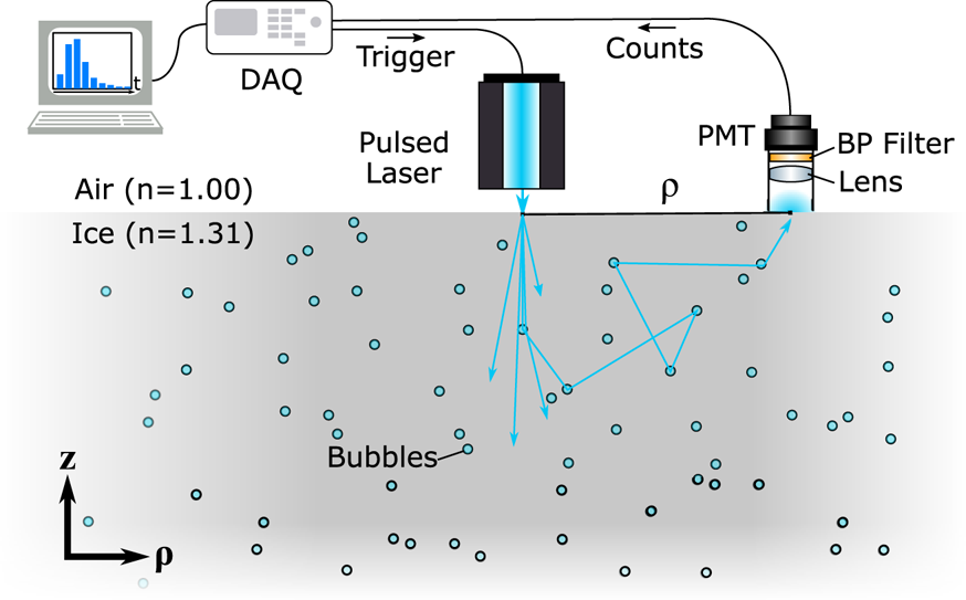
Fig. 1. The experimental setup is at its core similar to a photon counting LiDAR. The light source is a diode laser module, which emits pulses when triggered by the data acquisition module (DAQ). A delayed trigger pulse is used to gate the DAQ's counting circuit, which therefore only counts the events received from the photon counting detector in a discrete time interval after pulse emission. The arrival-time histogram is integrated in the LabView computer interface by shifting the delay between laser trigger and counter gate in constant time intervals. The backscattered light is collected onto the detector using a 50 mm-focal length lens and cleaned of most background light with a 10 nm-bandwidth bandpass filter. Both optical elements are inside a lens tube, which provides shielding from background. The photon counting detector is a photo-multiplier tube (PMT) with an active area 5 mm in diameter.
While this manuscript's focus is on measuring optical properties of bubbly glacier ice, the principle of the technique applies to any scattering medium. Here, we measure only effective scattering coefficients, which apply to an isotropic scattering process. The advantage of this approach is that assumptions about the nature of the scattering process and its distribution of scattering angles is not required. However, a discussion of the relationship between effective scattering coefficient and the physical mean-free path can give some context for different scattering media. For cold media – glacier ice, sea ice and snow – there are important differences for how the effective scattering length relates to established microscopic quantities. In bubbly ice, previous work assumed that the ice is solid with the refractive index being purely the one of ice. Scattering being dominated by bubbles of some average size and distance, which govern the mean-free-path of the physical scattering process (Price and Bergström, Reference Price and Bergström1997). Bubbles (similar to grains in snow) are assumed to be large compared to the wavelength of light. In reality, this scattering process is far from isotropic. Askebjer (Reference Askebjer1997); Price and Bergström (Reference Price and Bergström1997); Ackermann (Reference Ackermann2006) report a value of the average cosine of the polar scattering angle g = |cosθ| ≈ 0.75 for the case of Mie scattering on spherical bubbles, Kokhanovsky (Reference Kokhanovsky2004) report a value of 0.78 for the geometric contribution of scattering by ice spheres. It has been shown that any scattering problem in radiative transfer can be described through an effective, isotropic scattering process (Kokhanovsky, Reference Kokhanovsky2004), an approach that has been adopted by Askebjer (Reference Askebjer1997) and Ackermann (Reference Ackermann2006) as well. g then provides a convenient relationship between the physical mean free path l mfp and the effective scattering length l eff, which describes an effective, isotropic process:

The scattering length is the inverse scattering coefficient, l eff = 1/σeff and therefore

While scattering in near-surface ice is dominated by bubbles instead of cracks, dust and crystal boundaries (Price and Bergström, Reference Price and Bergström1997; Dadic and others, Reference Dadic, Mullen, Schneebeli, Brandt and Warren2013), these contributions may be significant close to the surface. For sea ice, liquid brine or salt crystals contained in the ice complicated things further since they can display a wide range of values for both their scattering cross-section and g (Light and others, Reference Light, Maykut and Grenfell2004). The advantage of measuring the effective scattering coefficient directly is that no assumptions about g or the nature of the underlying scattering processes need to be made.
Although the refractive index of glacier ice (in contrast to water ice containing no bubbles) depends on the volume fraction occupied by bubbles and therefore density, the same is true for the absorption coefficient (Dombrovsky and Kokhanovsky, Reference Dombrovsky and Kokhanovsky2020). With the absorptive component of the diffusion solution in Eqn (3) defined as β = c 0σabs/n, the density dependence of absorption coefficient and refractive index cancel.
3. Experimental methods
To measure the absorption and effective scattering coefficient of glacier ice, it is necessary to measure the fluence rate and fit the result with the diffusion theory from Eqn (5). The fluence rate describes how much energy flows through a unit area at arbitrary orientation per unit time. In our setup as shown in Figure 1 we inject a laser pulse vertically into the ice. The detector is placed in the scattering-far-field, in this specific case about 1.8 m away from the laser, which is of the order of ≈ 30l eff. A realistic detector has a finite area defined by the area imaged by the collection optics. Therefore, the appropriate function to use for a fit is the fluence rate integrated over this area, which possesses units of energy per unit time. Realistically, placing such a detector in the scattering-far-field introduces many orders of magnitude of loss (Allgaier and Smith, Reference Allgaier and Smith2021), which can only be overcome by using photon-counting detectors, a feature absent from most commercial LiDAR systems. At the same time, these detectors provide excellent temporal resolution.
While pulsed laser sources, photon counting detectors and the necessary timing electronics are all commercially available, not all varieties are affordable or appropriate. As shown in Allgaier and Smith (Reference Allgaier and Smith2021), the expected duration of the fluence rate distribution is between 100 and 1000 ns, which implies that a 10 ns-duration laser pulse is significantly shorter than the overall distribution, rendering it effectively ‘instantaneous’. The same is true for the employed electronics: The measurement can be implemented using the counter circuit of many data acquisition systems with ns-resolution. This option can offer sufficient resolution at comparatively lower cost.
We employ three different nanosecond-pulsed diode lasers (Thorlabs NPL41B, NPL52B and NPL64B emitting blue light at 405 nm, green at 520 nm and red at 640 nm, respectively) set to a pulse duration of 18 ns and a repetition rate of 1 MHz. All measurements are repeated with three different wavelengths. 405 nm is close to the absorption-minimum of ice (Warren, Reference Warren2019). 520 nm is close to the laser used by ATLAS onboard ICESat-2 (532 nm). The third laser at 640 nm serves as a reference. In transmission measurements, it has been assumed that the absorption coefficient of ice is mostly independent of LAPs at wavelengths longer than 600 nm. With the laser at 640 nm we can test this assumption. At a pulse duration of 18 ns the laser emits reasonable pulse energies (70pJ at 405 nm, 57pJ at 520 nm and 95pJ at 640 nm) without drastically diminishing the temporal resolution dominated by other components.
The detector is a photo-multiplier tube (PMT) module (Hamamatsu H7421-50) with an active area 5 mm in diameter. Scattered light is collected by a lens with NA = 2 (25 mm diameter, focal length 50 mm) and spectrally filtered with a 10 nm-bandwidth bandpass filter centered on each laser wavelength (Thorlabs), both placed in lens tubes which do not require alignment in the field. Compared with a lens as well as suing a lens tube provides additional shielding from background light. The detector has a quantum efficiency of 12% at 640 nm that outputs TTL pulses with a rise time of < 1.5 ns upon detecting a photon. The lens is set to focus collimated light onto the active area, effectively imaging an area 25 mm in diameter. Even with the bandpass filter in place, the photon-counting PMT module is saturated and possibly destroyed in daylight conditions. Therefore, measurements must be conducted after sunset.
In our setup, the time-resolved measurement is implemented using a data acquisition module (DAQ – National Instruments USB-6361). We use one counter circuit to generate a pulse train with a repetition rate of 1 MHz to trigger the laser. A second counter circuit is used to generate a pulse train that is synchronized to the first one except for a time delay. This second pulse train acts as a time gate for the third circuit which is used as an even counter. When gated, the counter circuit only counts events that arrive in the time window defined by the duration of the gate pulse. In this configuration, the fluence rate ϕ(ρ, T) can be measured as a function of delay T from the laser pulse launch time in a time interval of 20 ns, which is approximately equal to the input laser pulse duration. The measured time-of-flight (ToF) histogram is the average fluence rate in the measured time interval of 20 ns length. The complete ToF histogram is measured by stepping the delay T between the laser trigger and the counter gate pulse trains. With the temporal resolution of 20 ns (limited by the gate duration) and a pulse repetition rate of 1 MHz, we can resolve ToF distributions as short as a few time bins (one time bin being the gate duration of 20 ns), and as long as the time between two pulses (1000 ns). Since the laser is triggered externally using the DAQ, these parameters can all be easily adjusted in the field. With the laser repetition rate of 1 MHz, the time between consecutive pulses is 1000 ns, much larger than the dead time of the detector. In addition, the strong loss between the laser and detector guarantees that the number of detected photons per pulse is ≪ 1. This guarantees that the detector response in linear.
The histograms are evaluated with the native bin size of 20 ns as defined by the gate pulse duration of the DAQ. The last 5 bins (t = 900…1000 ns), which we can assume to only contain background, are averaged and the resulting background contribution is subtracted from all bins. Given laser-detector separation ρ (measured with a tape measure), Eqn (5) is then integrated over the time bin interval and fitted to the measured ToF histogram (Fig. 4 solid lines).
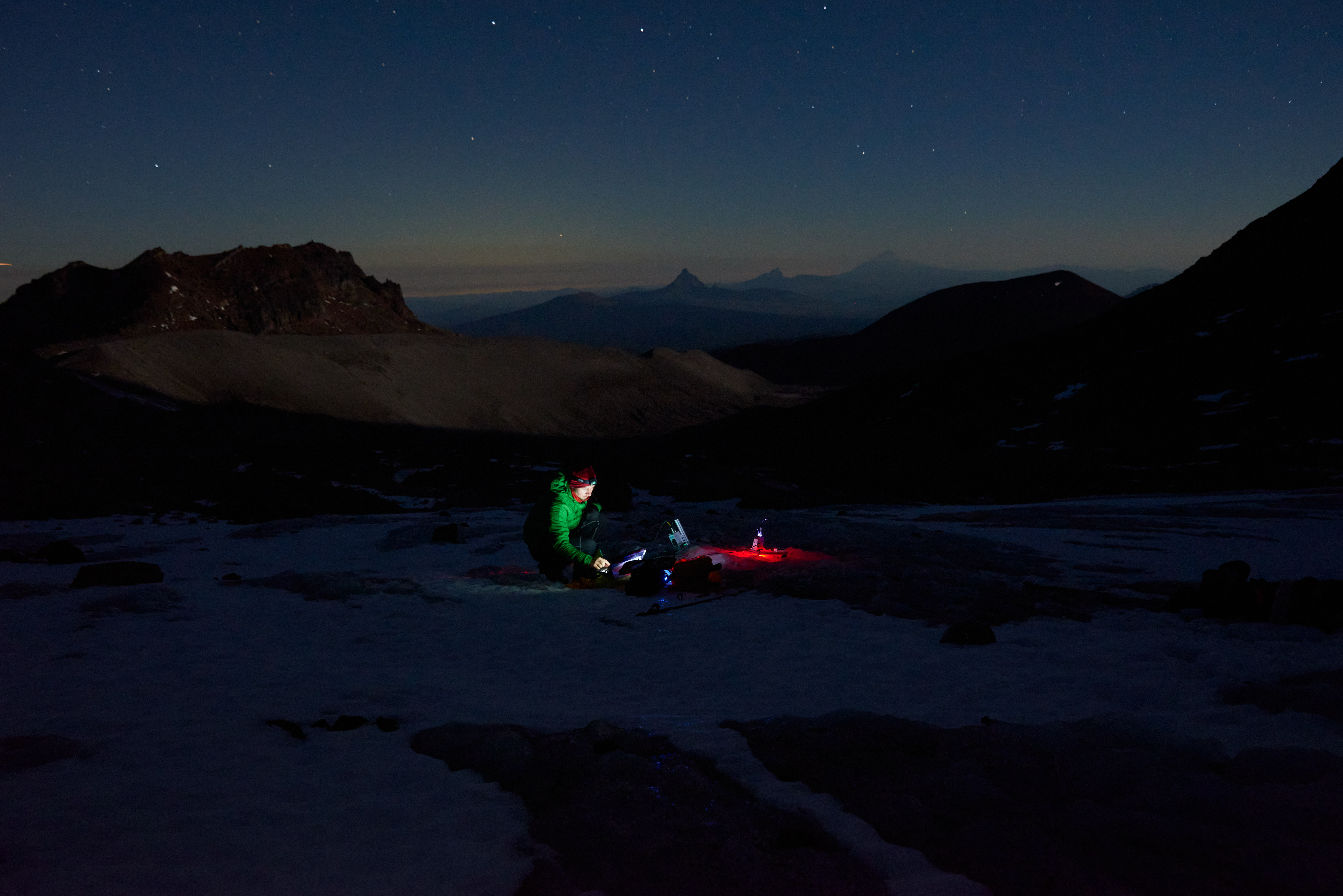
The setup does not need any alignment in the field and can be powered using a 200 Wh, 12 V battery for the DAQ and laser and a 50 Wh battery for the PMT (Goal Zero), which provide a runtime of ~10 h on the ice, rechargeable using portable solar panels. The DAQ is controlled using a LabView interface run on a tablet computer. The combination of being battery powered, using low-power (effectively class-1) lasers and transporting the instrument on foot ensures minimal environmental impact and enabled us to work in designated wilderness areas. Figure 2 shows the instrument in operation on Collier Glacier in the Three Sisters Wilderness, Oregon.

Fig. 2. Backscattered blue light can be seen right below the laser (a). The PMT is positioned to the left (b). A GPS receiver is co-located with the laser (c). The DAQ remains in its hard case (d).
In general, there are internal electronic delays between the different counter circuits, between laser trigger and optical output, as well as physical delays due to the length of cables. All of these need to be measured and subtracted from the measured ToF distribution to extract the ‘actual’ ToF. This is done by placing laser and detector close together and <30 cm away from a solid surface (scattering card or a wall) and measuring a ToF histogram. The actual ToF would be the physical path from the laser to the surface plus the distance from the surface to the detector, in this case <2 ns, unresolvable by the system. The peak at the measured distribution indicates the internal delay, which can then be subtracted from all measured ToF distributions. With the cables used here, the internal delay is 130 ns for all measurements taken on Collier Glacier and 190 ns for the calibration measurements taken on Crook Glacier.
A complete list of parts required to build this setup and further explanation of the timing circuitry can be found in Appendix A.
4. Study area
Field work was conducted on Collier Glacier located in the Three Sisters Wilderness, Oregon, USA (see Fig. 3). Collier Glacier is a temperate valley glacier in Oregon with an elevation of between 2300 and 2700 m and an area of ~0.7 km2 (Mountain, Reference Mountain1978; Beedlow, Reference Beedlow2011). Data were collected at two sites (44.169444°N, 121.788256°W, 2324 m and 44.167509°N, 121.784424°W, 2406 m, respectively) on 24 and 25 September during which the glacier was mostly free of snow, with only the crevasses and upper-glacier being covered by a recent layer of snow (the measurements were made on bare ice).

Fig. 3. The study area on Collier Glacier, Three Sisters Wilderness, Oregon. Two sites were sampled: one close to the northern terminus, and one in the middle of the glacier, below the ice fall which roughly marks the average ELA.
Data collection was performed during two nights starting about 1 h after sunset (20:00) when the background light level had subsided sufficiently as to not saturate the PMT. At each site, 8–10 measurements at each wavelength (405, 520 and 640 nm, 30 measurements total at each site) were taken over the course of 3–4 h each night, with the initial setup taking not more than 15 min. For these measurements, the laser and detector were moved to different positions on an area of 4×6 m, where the distance between laser and detector was kept between 1.5 and 1.9 m, determined with a tape measure. All measurements were completed for one wavelength before moving on to the next. This order is preferable over taking three measurements at different wavelengths at the same location, because the laser head needs several minutes to warm up and achieve constant output power.
In addition to the measurements on Collier Glacier, a series of measurements aimed at determining optimal distance between the laser source and the detector was conducted on 16 September on the nearby Crook Glacier (44.079917 N, 121.698415 W, 2506 m), which unlike Collier Glacier widely lacks reference data from previous research but offers far easier access. On Crook Glacier, the laser mount was kept in the same position throughout the night, swapping the laser heads in place to ensure that measurements at different wavelengths were comparable. The detector was moved to distances from the laser between 0.8 and 2.5 m with the goal of establishing a useful distance range in which ToF histograms could be measured with a reasonably well-resolved peak (histogram occupying at least 5–6 bins) and sufficient signal-to-noise ratio (SNR – at least 1000 counts per bin after background-subtraction).
5. Results
5.1 Data analysis
To analyze the measure ToF histograms, Eqn (5) is used to perform a least-square fit. The theoretical model is amended by a multiplicative scaling constant C as well as a timing offset:

with C, σeff, σabs, Δt as fit parameters. While in theory, the absolute arrival time offset Δt should be zero, we can only characterize it with the limited resolution of the time-resolved counter (20 ns). We hence include it as a fit parameter. Eqn (8) is additionally integrated over each 20 ns bin in the measured ToF histogram (see Fig. 4). This integrated value is what is compared to the data in the least-square fit routine.
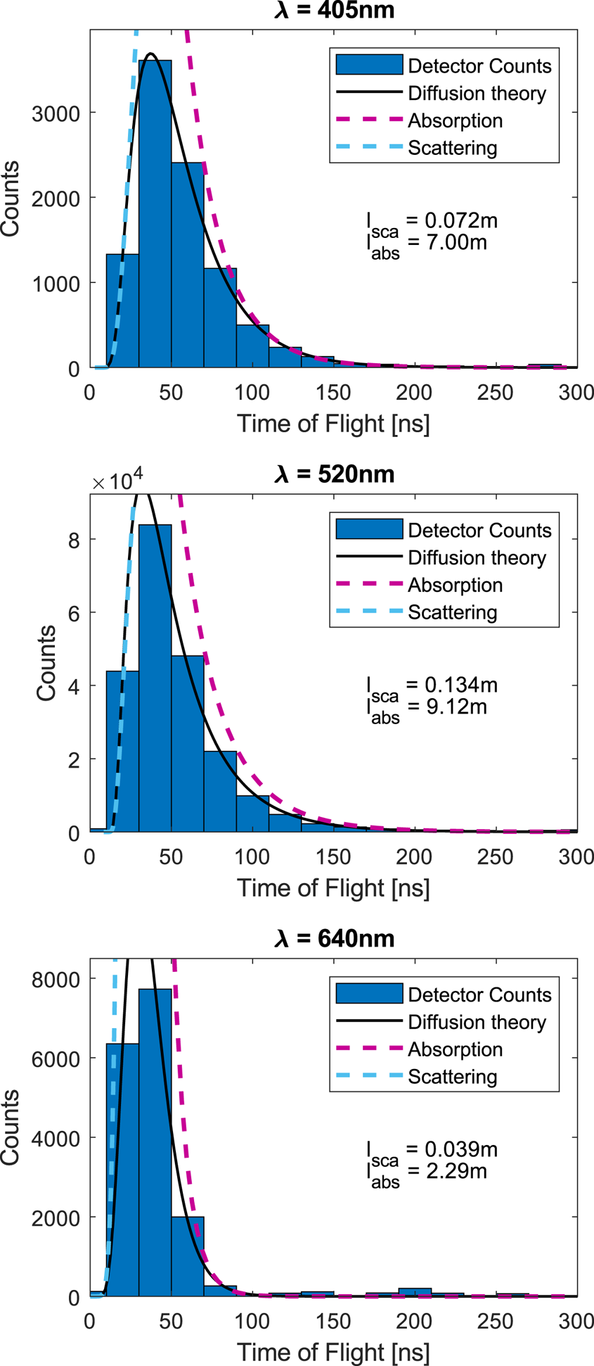
Fig. 4. Arrival-time histograms for the three different wavelength as recorded on Crook Glacier. Blue bars represent the background-subtracted data. The solid black line is the fitted diffusion curve, from which absorption and scattering coefficient are extracted. The cyan and magenta dashed lines are the diffusion curve with the absorptive and scattering component, respectively, turned off.
5.2 Characterization at optimal laser-detector separation
Measurements taken on Crook Glacier indicated that the appropriate distance between laser source and detector was between 1.5 and 2 m. Below 1.5 m, the peak of the ToF histogram was poorly resolved due to insufficient temporal bin width, especially for the red 640 nm-laser, where absorption is stronger. Above 2 m, ToF histograms were increasingly hard to measure, with the required integration time exceeding 10 min accompanied by poor SNR. Note that the laser mount was left in place to keep alignment constant, which is necessary to compare measurements at different wavelengths.
For the ideal separation, we show three ToF histograms recorded at a distance of 1.4 m in Figure 4. The figure also shows that same result of the fit with the absorptive and scattering component turned off, respectively (cyan and magenta dashed lines, respectively), re-scaled for better visibility. This shows that the rising edge of the distribution is governed mostly by the scattering coefficient, and the falling edge and slow fall-off is where the absorption coefficient is extracted. With identical laser position, all three measurements yield scattering coefficients of 14(±4), 7(±2) and 29(±7)m−1, respectively for 405, 520 and 640 nm, where we assume a relative uncertainty of 25%, derived from the reliability of the curve fit on simulated data (Allgaier and Smith, Reference Allgaier and Smith2021). The absorption coefficients extracted from the fitted curve (0.14(±0.04), 0.11(±0.03) and 0.5(±0.1)m−1, respectively for 405, 520 and 640 nm) are in the range of literature values (Warren and Brandt, Reference Warren and Brandt2008).
It can, however, be seen that the peak is poorly resolved at 640 nm, which can be attributed to the strong absorption at that wavelengths, resulting in a truncated peak structure, which does not change as a function of distance. We would require higher temporal resolution to resolve the peak at 640 nm. At smaller separation, the peak onset is poorly resolved at all wavelengths. At separations larger than 2 m, histograms are exceedingly hard to measure, requiring large integration times. Therefore, we conclude that the ideal distance between detector and laser source for the study area is between 1.5 and 2 m. Overall, our instrument successfully retrieved both scattering and absorption coefficients through successful curve fits for 405 and 520 nm, where both the peak onset and the tail of the distributions are well resolved. Shortcomings particularly in the parameter retrieval at 640 nm will be discussed in the following section.
5.3 Statistical independence of scattering and absorption coefficients
To judge the quality of the obtained curve fits, we vary each of the four fit parameters for the data shown in Figure 4 around the respective values obtained from the fit and calculate the χ2 (sum of the square deviations). The resulting χ2-landscapes are shown in Figure 5. The panels in the first column (a, d, g) show the χ2-landscape for the combination of scattering and absorption coefficient (with the other two fit parameters held constant) for the three previously shown fits. For the data obtained at 405 and 520 nm (panels a and d), the χ2-landscape constrains the fit values in both directions. The 405 nm data exhibit a slight anti-correlation. The data for 640 nm on the other hand (panel g) show this anti-correlation in a much more severe way, as the absorption and scattering coefficients are not independently constrained within the plotted window of $\pm 5\percnt$ around the fit values. This implies that we cannot retrieve independent value for the absorption and scattering coefficients from such poorly resolved data. The second column (panels b, e, h) show the same plot but for the combination of absorption coefficient and the multiplicative scaling factor. These tend to show anti-correlation, however, the same is true for the scaling factor and scattering coefficient, which are shown in panels (c, f, i). Therefore, the scaling factor correlates identically with both the absorption and scattering coefficient, implying that all are well constrained in a fit where they are all free parameters.

Fig. 5. Sum of square errors in units of W2m−4 between fit and data for the parameter space around the best-fit-values extracted from the histograms shown in Figure 4. Panels (a, d, g) show the sum of least squares for combinations of different values for the effective scattering and absorption coefficients with the other two parameters kept constant for the histograms recorded at 405, 520 and 640 nm, respectively. Panels (b, e, h) show the same data for the scaling constant and absorption coefficient. Panels (c, f, i) are for the combination of scaling coefficient and scattering coefficient. The scale of the colorbar is identical within each row.
Particularly the fit behavior for the two important optical parameters in question here, scattering and absorption coefficient, is well constrained and therefore the fit should yield an independent value for both. Therefore, weak correlations like what the one shown in Figure 5a will not manifest. This is not true for the data taken at 640 nm, where the fit has to be assumed to be less reliable. This will become evident as we examine correlation between many different data points in the following.
In practice, there should be no correlations between the physical scattering and absorption coefficients found in typical surface glacier ice, where scattering is mostly due to bubbles, and absorption is dominated by LAPs. To test this assumption, a large and diverse dataset is needed to ensure that there are no such correlations in the underlying coefficients. For this purpose, we combine the data measured at both sites on Collier Glacier as well as the Site on Crook Glacier. Given the χ2-study, we interpret the data measured at 405 nm (blue) and 520 nm (green) separately from the one taken at 640 nm (red). The fits for all histograms were unsupervised using identical initial parameters. A scatter plot of the successful measurements is shown in Figure 6.
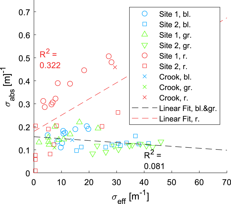
Fig. 6. All combined data points for scattering and absorption coefficients from both Crook and Collier glaciers at all three wavelengths. The dashed black line represents a linear fit to blue and green data (R 2 = 0.081), which illustrates the statistical independence of the retrieved parameters. The red dashed line (R 2 = 0.323) represents the linear fit to red data.
To establish whether the extracted value pairs are statistically independent or not, we perform a linear fit and calculate the R2 of the distribution. For blue and green data combined, we find R 2 = 0.081, while it is 0.323 for the red data. This demonstrates that a linear best fit represents the distribution no better than a simple average in the blue and green, however, there is a clear correlation between absorption and scattering in the red dataset. We therefore conclude that this method can indeed provide an independent measurement of scattering and absorption coefficient as long as ToF histograms are well resolved, as is the case at 405 and 520 nm. However, this is not true for data taken at 640 nm, where insufficient resolution manifests both in a larger spread of the measured values as well as clear correlations between the two coefficients.
5.4 Results from Collier Glacier
The extracted scattering and absorption coefficients for the two sites are shown in Figure 7. Thicker symbols represent the mean coefficient pair at each wavelength, with the error bars representing the standard deviation. We use the standard deviation as a conservative estimate of the measurement uncertainty, as the observed spread encompasses both uncertainty from the model fit and natural variations of the glacier ice properties. First, it can be seen that the scattering coefficients for the green and blue wavelength, for which the peaks of the ToF distribution are generally well resolved, are comparable at each of the two sites. The red scattering coefficients seems at Site 2 to be significantly different from the others. This is also true when we average the coefficients over both sites (20.9(±1.5), 22.2(±3.0) and 11.9(±2.6)m−1 at 405, 520 and 640 nm, respectively), where the stated uncertainties are standard errors. While the values at 640 nm differ significantly from the others, it is still within a 2σ uncertainty range. That said, we emphasize that the scattering coefficient measured at 640 nm suffers from poor temporal resolution, which implies that the scattering coefficient may be underestimated (compare Site 2).

Fig. 7. Scattering and absorption coefficients from the two sites on Collier Glacier with blue circles, green triangles and red circles representing data taken at 405, 520 and 640 nm, respectively. Thick symbols are the mean scattering and absorption coefficient for each wavelength, and the error bars representing the standard deviation of each distribution.
The extracted absorption coefficients provide a more uniform picture. Average values at 405 and 520 nm are almost identical and, as expected, red absorption is stronger than green and blue. The absorption coefficients (10−1m−1) are at the upper end of the range of previously published values (Warren and Brandt, Reference Warren and Brandt2008) (c.f. Fig. 12 of Cooper and others (Reference Cooper2021)), suggesting that the ice we measured at Collier Glacier contained substantial concentrations of BC or other LAPs. Such large coefficients and the fact that the absorption is almost identical for the green and blue part of the spectrum agree with observations made on icebergs and glacier ice contaminated with algae and organic LAPs (Warren and others, Reference Warren, Roesler, Brandt and Curran2019b). The fact that the absorption coefficient at Site 2 is lower than it is on Site 1 would also indicate a larger albedo, consistent with previous observations on Collier Glacier, where the broadband albedo was found to be lower at the terminus (Mountain, Reference Mountain1978).
While previous work often considered the absorption coefficient at wavelengths >600 nm to be independent of LAPs, it is apparent from simulations of snow albedo that this is only true for small concentrations (Warren and Wiscombe, Reference Warren and Wiscombe1980). However, due to its smaller scattering coefficient, ice albedo would depend more strongly on the absorption coefficient and LAPs. We will elaborate on this aspect in the next section for the example of BC.
To summarize, the observed absorption coefficients are consistent with glacier ice contaminated by LAPs, which is to be expected for any glacier outside of the Arctic or Antarctic.
5.5 Penetration depth, albedo and LAP concentration
Our measured scattering and absorption coefficients are relevant to a number of different applications, including inference of laser altimeter penetration depth, albedo and LAP concentrations. Firstly, the effective scattering length represents the depth at which the direction of scattered photons has been fully randomized. In the limit of small absorption, this is the approximate depth at which a maximum of backscattering to the surface occurs. In the context of laser altimetry or LiDAR mapping, this can be interpreted as the penetration depth. Averaged over both sites, the scattering length at 520 nm (close to common wavelengths for LiDAR systems) is 6.9 cm, meaning that LiDAR measurements taken at nadir need to account for such a bias. Our measurements can be considered a first-order approximation of this bias, but more work is needed to quantify the magnitude and variability of this bias over different surfaces and to understand effects such as pulse broadening.
Secondly, it has been shown that the radiative transport for bubbly glacier ice can be framed in terms of effective bulk scattering and absorption coefficients (Dombrovsky and Kokhanovsky, Reference Dombrovsky and Kokhanovsky2020) like the ones measured here. To this end, we first define the effective single-scattering albedo ω = σeff/(σeff + σabs). Since the refractive index of ice n is larger than that of air, total internal reflection occurs for upwelling radiation impinging on the air-ice-interface at angles larger than $\mu _c = \sqrt {1-( 1/n^2) }$ . Dombrovsky and Kokhanovsky (Reference Dombrovsky and Kokhanovsky2020) then define the following parameters needed to express the reflectance function:

where R(1) is the Fresnel reflection coefficient at normal incidence. The plane albedo r p then reads

where μi is the cosine of the incidence angle.
Note that this equation takes into account a specular surface reflection. Using this expression we can calculate the plane albedo for any angle of incidence. We extrapolate the measured spectral components from 405 to 640 nm into the UV and IR and assume that the absorption coefficient is independent of LAPs outside of the visible range (Warren and Brandt, Reference Warren and Brandt2008). Then, we take the average of the measured scattering coefficients to calculate a complete spectral albedo curve. The results for an incident angle of 60° are shown in Figure 8, where reduction in spectral albedo throughout the visible spectrum from Site 2 to 1 is visible. We also show the spectral albedo assuming clean ice and measured scattering coefficients. To estimate a broadband albedo at each site, we calculate a weighted average of the spectral albedo, using a solar spectrum calculated with COART (Jin and Stamnes, Reference Jin and Stamnes1994) as a weight. Values obtained in this way are 0.48±0.03 and 0.56±0.03 for Site 1 and 2, respectively, and 0.62 assuming clean ice.

Fig. 8. Spectral albedo on both sites as well as for clean ice. Data points at 405, 520 and 640 nm are calculated from measured scattering and absorption coefficients (open circles). Other data points are calculated from literature values for absorption and the averaged measured scattering coefficient (open squares). Solid lines represent linear interpolation as a guide to the eye. The dashed line was calculated using absorption coefficients for clean ice and the scattering coefficients from Site 2.
Although established methods from reflectance spectroscopy provide measured spectral albedos, such techniques typically only answer the question what the albedo is. In contrast, our method provides the underlying absorption and scattering length scales that explain why albedo assumes a particular value, and decouples absorption and scattering properties, thus eliminating the need for further measurements of structure or composition.
Lastly, we use the measured absorption coefficient to estimate effective concentrations of LAPs. For this, we require a baseline absorptivity for clean ice. One such estimate by Warren and others (Reference Warren, Brandt and Grenfell2006) gives a value of σabs,clean = 7.78×10⁻⁴m−1, while Picard and others (Reference Picard, Libois and Arnaud2016) gives a more conservative estimate of σabs,clean = 1.9 × 10⁻² m−1 at 405 nm. We will give results using both reference values. The density d = 870 kg m−3 has been measured using an ice screw with a diameter of 1.3 cm and length of 15 cm as a sampler. For this demonstration, we assume that BC is the only LAP, which implies that extracted concentrations are an upper bound. We assume an Angstrom coefficient of 1.1 and a mass absorption cross-section of C BC = 8.9 m2g −1 at λref = 450 nm (Doherty and others, Reference Doherty, Dang, Hegg, Zhang and Warren2014). Using these values the concentration can be calculated using

For the two sites and using the clean ice absorption value from Warren and others (Reference Warren, Brandt and Grenfell2006), this yields BC concentrations of 18.9(±3.5) and 14.1(±1.9) ppb, respectively. Using the clean ice absorption measured by Picard and others (Reference Picard, Libois and Arnaud2016) instead, the measured concentrations emerge as 16.8(±3.5) and 12.0(±1.9) ppb, respectively, for the two sites. These values are well within the range of values previously reported for the region which lie between 6 ppb in Washington State and 156 ppb in Eastern Oregon (Doherty and others, Reference Doherty, Dang, Hegg, Zhang and Warren2014) and in summer snow on Mount Olympus, Washington State (Kaspari and others, Reference Kaspari, McKenzie Skiles, Delaney, Dixon and Painter2015). It appears that different reference values influence the accuracy of such a measurement for smaller concentrations. For concentrations > 20 ppb, this should not change the percent difference in inferred LAP concentration by nearly as much as in cleaner ice. Although future work is needed to validate this estimate from laboratory analysis of ice from Collier Glacier, the range of values obtained demonstrates the utility of the measurements and the principle of the method. That said, laboratory analysis of LAP content and debris in snow and ice also suffers from limitations, with part of the particulate mass often not accounted for in dust and BC analysis. This leads to large uncertainty in the apparent optical properties estimated from laboratory analysis, further highlighting the utility of quantifying absorption independently from scattering. Both pathways – estimating LAP content from measurement of optical properties and estimating optical properties from LAP content – ultimately rely on precise knowledge of the mixing ratio and optical properties of each LAP. With the tight grouping of measured absorption coefficients shown in Figure 7, the technique presented here could provide reasonably accurate estimates of LAP concentrations in the field. This is particularly important for diagnosing cryospheric change in remote locations, where retrieval of ice cores and physical samples is logistically difficult and costly, and therefore presents a unique opportunity to simplify data collection. It is notable that bare ice albedo appears more sensitive to LAPs than snow, an effect that has been observed for sea ice as well (Marks and King, Reference Marks and King2013).
In summary, there are several valuable metrics that can be inferred from measured absorption and scattering coefficients. Since these measured values are effective properties of the bulk, no additional knowledge about the physical structure or assumptions about LAP content are needed, making these calculations particularly simple.
6. Discussion
We have shown that the portable instrument presented here can resolve photon ToF histograms in temperate, near-surface glacier ice. While this process works for short visible wavelengths at 405 and 520 nm, where analysis of the model fit performance revealed that the scattering and absorption coefficients are well constrained, this is not the case for the data measured at 640 nm within the constraints of the temporal resolution of our experimental setup. Here, the ToF histograms are poorly resolved, which introduces significant correlations and poor accuracy in the retrieved parameters. Therefore, the data taken at 640 nm presented here are of limited quality and need to be interpreted as such. Improvements in temporal resolution would be desirable for red and infrared light. This concerns both the actual measurement resolution (currently 20 ns) as well as the laser pulse duration of 18 ns, which could be improved using commercially available means. For most data taken at 405 and 520 nm shown here, measured ToF histograms are of sufficient quality to extract optical scattering and absorption coefficients of bare glacier ice. While measurements taken at 640 nm are at the temporal resolution limit, impairing retrieval of the scattering coefficient, improved resolution could be enabled with a time-to-digital converter or electronics based on a field-programmable gate array. While additional improvements such as a laser with higher pulse energy or shorter pulse duration would further reduce measurement duration and increase resolution and SNR, they would also increase cost. In addition to improvements in terms of resolution, validation of extracted LAP concentrations from laboratory measurements would be beneficial to evaluate the viability of using optical measurements as a proxy for LAP concentration. The same goes for bubble size distribution and concentration, which would help set bounds on the measured scattering coefficients. Another open question lies in the response of the measurement to inhomogeneities in the ice, which is not obvious from evaluating the current data set alone.
The coefficients measured here are near the upper end of the range of previously reported values in the literature (Cooper and others, Reference Cooper2021), which implies that our setup can resolve ToF histograms on glaciers with similar composition. For clean ice characteristic of polar regions, reported absorption coefficients of near-surface ice are smaller but, along with scattering coefficients, may exhibit greater spatial variability associated with greater range of ice histories exposed at the surface. For example, differences between the scattering and absorption coefficients of deep ice melting out near the terminus of large glaciers and ice sheets relative to younger ice near the equilibrium line altitude may be explainable in terms of a common age or ice provenance. Therefore, the ToF histogram approach presented here could provide additional context for optical coefficients measured by others in Greenland (Cooper and others, Reference Cooper2021) and Antarctica (Ackermann, Reference Ackermann2006), and could provide the basis for a systematic investigation of underlying structural controls on ice-sheet albedo, which has been identified as a measurement priority needed to improve albedo parameterizations in large-scale models (Dadic and others, Reference Dadic, Mullen, Schneebeli, Brandt and Warren2013).
Direct measurements of optical properties eliminate assumptions about structure and composition of ice. The simultaneous measurement of scattering and absorption properties allows us not only to infer LAP concentrations and albedo, but also to link these surface optical properties directly to the underlying features in composition and structure. With this complex set of parameters derived from a single measurement, it becomes possible to better understand the optical properties of bare ice and build useful albedo models. In addition, albedos inferred from scattering and absorption coefficients can be interpreted in terms of structure and composition, which cannot easily be done with albedo measurements alone. They in fact lie on the higher end of the range of previously reported absorption coefficients, which is expected for a mid-latitude glacier, where concentrations of LAPs can be expected to be higher than in the Arctic or Antarctic regions. An example is the dependence of bare ice albedo on LAP concentration illustrated here: As the scattering coefficient is lower in bare ice as compared to snow, the dependence of the albedo on the absorption coefficient is stronger, making glacier ice albedo much more susceptible to LAPs. We observe significant albedo lowering of 0.07 from a difference in BC concentration of only 6 ppb. In snow, such drastic lowering of the broadband albedo would require BC concentrations of several 1000 ppb (Warren and Wiscombe, Reference Warren and Wiscombe1980). In conclusion, albedo of higher density ice with lower bubble concentration like that found in the Greenland ablation zone (Cooper and others, Reference Cooper2021) would be highly susceptible to even small concentrations of LAPs.
Knowledge of the optical properties of glacier ice is needed to understand LiDAR interactions with snow and ice, including penetration depth. In addition, it has been shown that precise measurement of the directional dependence of the scattering coefficient can potentially identify the average crystal C-axis orientation and therefore flow direction (Aartsen and others, Reference Aartsen2013; Katlein and others, Reference Katlein, Nicolaus and Petrich2014; Rongen and others, Reference Rongen, Bay and Blot2020; Rongen and Chirkin, Reference Rongen and Chirkin2021). All this information can be made available in the field including rugged, remote terrain, reducing the need for sample shipping and off-site analysis, which could provide significant savings in cost and simplify expedition logistics. The non-invasive and small footprint nature of the instrument allows for deployment in remote areas such as the United States federally designated Wilderness Areas, where motorized access and invasive measurement techniques are typically prohibited.
With more advanced techniques for photon-counting LiDAR such as photon-number threshold detection on the horizon (Cohen and others, Reference Cohen2019), we hope to further improve the sensitivity to the point where it becomes possible to resolve the small scattering contributions of LAPs and dust. The individual behavior of contributions such as dust has only recently been measured (Cremonesi and others, Reference Cremonesi2020), enabling us to potentially include such behavior into our model.
Supplementary material
The supplementary material for this article can be found at https://doi.org/10.1017/jog.2022.34.
Data availability
The raw data for all ToF histograms along with the code required to evaluate them and extract scattering and absorption coefficients are available at https://doi.org/10.5281/zenodo.5828621.
Code availability
The code used for evaluating each ToF measurement is published alongside the raw data at https://doi.org/10.5281/zenodo.6262752. The LabView interface used to perform the measurement can be found at https://doi.org/10.5281/zenodo.5828379. An online version of the COART code used to simulate the solar spectrum used in the broadband albedo calculation is available at https://cloudsgate2.larc.nasa.gov/jin/coart.html.
Acknowledgements
This work was supported by the University of Oregon through the Renee James Seed Grant Initiative. We thank Nicolas Bakken-French, Kyle Strachan and Jon Meyers for their help with field work. We thank the reviewers for their detailed and helpful comments, particularly on the data analysis procedure, which one reviewer had implemented themselves.
Appendix A. List of parts
Lasers. Thorlabs NPL41B, NPL52B, NPL64B
Detector. Hamamatsu H7421-50 (most photon-counting PMTs can be used for this purpose)
Optical elements. 50 mm focal length, 25 mm diameter lens, anti-reflection coated for visible light: Thorlabs LA1131-A
10 nm-bandpass filters: Thorlabs FB405-10, FB520-10, FB640-10
Lens tubes: Thorlabs SM1L10
Data acquisition. National Instruments USB-6361 with BNC breakout block (any NI USB-63xx series DAQ has the same counter functions necessary to run the LabView code).
Cables. RG58 cables with BNC connectors
3 dB attenuator for laser triggering
GPS receiver. Garmin GLO 2
Cost. The total cost is ~7000 USD, assuming a more modern PMT is used.
Appendix B. Time-of-flight measurements using NI data acquisition modules
The NI DAQs have so-called ‘counters’, which can either count edges of TTL (5 V square) pulses on a specified input or act as pulse generators. To facilitate a time-of-flight measurements, we use three counters. Counter 0 generates a pulse train of predefined repetition rate and is supplied to an output, which is connected to the trigger input of the laser. Internally, the frequency output from Counter 0 is routed to the trigger input of Counter 1, which also generates a pulse output, synchronized to Counter 0. The output pulse length of the output of Counter 1 is equal to the desired gate length (time bin size). An artificial delay is applied between the trigger input from Counter 0 and the pulse output from Counter 1 which corresponds to the start time of the current time bin. The third counter, Counter 2, works as an edge counter for the pulses coming from the photon-counting detector. The pulse train from Counter 1 is internally routed to the gate input on Counter 2. To record the entire ToF histogram, the delay on the pulse output of Counter 1 needs to be step-wise increased.
Alternatively, if the laser can operate as a stand-alone pulsed source without external input, it can be used as a frequency master for the whole system. The laser needs an output, which provides a trigger signal whenever the laser fires. This trigger is then routed to an input on the DAQ. This input is then used to trigger a pulse train on Counter 0, with a pulse duration equal to the desired gate length (time bin size). The frequency output from Counter 0 is internally routed to the Gate Input on Counter 1, the TTL signal from the photon counting detector is routed to the input of Counter 1. The artificial delay between the trigger input and the output of Counter 0 corresponds to the start time of the current time bin and needs to be increased step-wise to build a complete ToF histogram. With the lasers used here, this solution would work for repetition rates of 1 MHz or faster, which the laser can produce without external trigger. In this configuration, a cheaper data acquisition module with only two counter circuits would suffice, but the setup would sacrifice the flexibility to use slower repetition rates which are required to record long ToF distributions as they would manifest for high-density, clean ice. This use of the DAQ is similar, but not identical to the ‘pulse separation’ measurement described in the manual, which imposes further constraints on photon detection rates.
In both counter configurations, the repetition rate should be chosen so that the entire ToF distribution is captured and the measured intensity falls to the background count rate by the end of each cycle. The temporal bin size Δt can be chosen as small as two cycles of the counter circuit's clock frequency νclock:

Appendix C. Approximate determination of the scattering-far-field ‘by eye’
As a first approximation, the optical distance between source and detector can be determined ‘by eye’, as the intensity falls off as a function of distance from the laser (see Eqn (33) in Allgaier and Smith (Reference Allgaier and Smith2021)):

In ice, this exponential fall-off is dominated by the scattering coefficient, which is much larger than the absorption coefficient. A reduction in intensity of one order of magnitude corresponds to a distance of about three scattering lengths. As a simple approximation, the detector should be placed outside the area of visible backscattered light, ensuring several orders of magnitude in intensity reduction. However, if this distance is too large, there will be little backscattered light, reducing SNR. For small distances, arrival times will also be shorter according to Eqn (5), meaning that temporal resolution may not be sufficient to resolve the arrival time distribution appropriately.


 Open access