


Introduction
Building and construction require bulk amounts of aggregate (granular mineral material), produced from natural sand, gravel or solid rock resources. The Netherlands is one of the most densely populated nations in the world, with very high land use intensity. More than in most other countries, aggregates extraction interferes with existing or planned land use, and is often controversial. Because of this, access to Dutch aggregate resources is considered in integral spatial planning, rather than being secured through some specific minerals policy instrument (e.g. production planning; van der Meulen, Reference van der Meulen, Petterson, McEvoy and Marker2005; van der Meulen et al., Reference van der Meulen, Broers, Hakstege, Pietersen, Van Heijst, Koopmans, Wong, Batjes and Jager2007a).
Integral spatial planning is based, amongst other criteria, on the evaluation of land use potential, and in the case of aggregates extraction it is obviously resource presence and quality that need to be considered. On regional to national scales, such information is usually provided by geological survey organisations. Since 2005, aggregate resource assessments made by the Geological Survey of the Netherlands have been based on voxel models, voxels being attributed volume cells in a rectangular 3D grid (3D pixels). So far, three such assessments have been carried out. The first two have national coverage (van der Meulen et al., Reference van der Meulen, van Gessel and Veldkamp2005, Reference van der Meulen, Maljers, van Gessel and Gruijters2007b; TNO, 2014a) and the third is derived from the Survey's ongoing multipurpose national 3D modelling programme GeoTOP (Stafleu et al., Reference Stafleu, Maljers, Gunnink, Menkovic and Busschers2011, Reference Stafleu, Maljers, Busschers, Gunnink, Schokker, Dambrink, Hummelman and Schijf2012). All three models are primarily based on borehole data. Progress has been made in the extent to which additional soft data have been taken into account, such as lithostratigraphic interpretations, geological map data and lithofacies concepts. In addition to that, ever-increasing computer performance enabled us to produce each new model at a higher resolution.
While our 3D models became evermore detailed and geologically realistic, the development and production costs of these models rose by approximately two orders of magnitude. Using aggregate resource estimation as a test case, the present contribution discusses the progress made in our modelling efforts from a geological perspective (How geologically appealing was each model?) balanced against the effort and application possibilities (Did each improvement make the model better fitted for the purpose?). As we aim to qualitatively describe actual progress in 3D modelling, we left the voxel models as they were when they were constructed. We rechecked and fine-tuned our resource calculations on the basis of the three models to achieve as much consistency as possible for our comparisons.
Although the authors adhere to its basic principles, this study does not formally comply with the current reporting conventions (Anonymous, 2001, 2008; see also Anonymous, 2004). Our results are not to be used for the purpose of (a) informing investors or potential investors and their advisers or (b) satisfying regulatory requirements.
Geological setting
Our study area, 40 × 40 km, is located in the central Netherlands and includes a section of the Rhine-Meuse delta and adjacent glacial terrains (Fig. 1). For the reasons outlined below the area is particularly suited for the evaluation at hand. It is large enough to include all relevant features to evaluate aggregate resource and produce resource statistics, and small enough to oversee and illustrate the differences between the models. Our primary comparisons were made down to 30 m below the surface, as aggregate extraction usually does not exceed this depth.
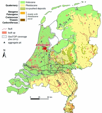
Fig. 1. Geological map of the Netherlands showing the location of the study area (A) and the proportion of the country with GeoTOP coverage (other models referred to in the text are nationwide). The study area is located in GeoTOP Rivierengebied (see text for explanation). The area marked (B) is discussed in detail; the cross-section line (C) refers to Fig. 2. RVG, Roer Valley Graben.
The Pleistocene in the delta area in the depth range of interest consists mainly of fluvial deposits of the rivers Rhine and Meuse (Waalre, Stramproy, Sterksel, Urk and Kreftenheye Fms; Busschers et al., Reference Busschers, Weerts, Wallinga, Kasse, Cleveringa, De Wolf and Cohen2005, Reference Busschers, Kasse, van Balen, Vandenberghe, Cohen, Weerts, Wallinga, Johns, Cleveringa and Bunnik2007; all stratigraphic units cf. de Mulder et al., Reference de Mulder, Geluk, Ritsema, Westerhoff and Wong2003; Fig. 2). The units vary lithologically and in fluvial style, which is ultimately controlled by the tectonics and hydrology of the Rhine and Meuse catchment areas, base-level variation and climate (especially through glaciations; Berendsen & Stouthamer, Reference Berendsen and Stouthamer2000; Busschers et al., Reference Busschers, Weerts, Wallinga, Kasse, Cleveringa, De Wolf and Cohen2005, Reference Busschers, Kasse, van Balen, Vandenberghe, Cohen, Weerts, Wallinga, Johns, Cleveringa and Bunnik2007; Gouw, Reference Gouw2007; Gouw & Erkens, Reference Gouw and Erkens2007). The dominant lithology is medium to coarse, occasionally gravely sand, but clay also occurs, especially in the older units. The sequences are generally coarsening upward.
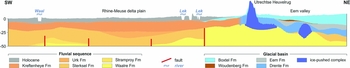
Fig. 2. Cross-section through the study area based on DGM (Gunnink et al., Reference Gunnink, Maljers, Gessel, van, Menkovic and Hummelman2013; see text for explanation). For location see Fig. 1.
During the penultimate (Saalian) ice age, the northeast corner of the study area was overridden by an advancing ice sheet. An ice-pushed ridge was formed (the Utrechtse Heuvelrug), of which the sandr fans (Drente Fm) interfingered with the fluvial systems that persisted in the south (Kreftenheye Fm). The ice-scooped basin behind the Utrechtse Heuvelrug, the Gelderse Vallei, was filled initially by fluvio-glacial and proglacial deposits (Drente Fm). During the Eemian highstand the area was inundated by the sea, as evidenced by a body of shallow marine clays that is present at depths between 10 and 25 m, followed by coastal peat (Eem and Woudenberg Fms, respectively). At the beginning of the Weichselian ice age, sea level dropped and fluvio-glacial sedimentation resumed (Boxtel Fm).
Glacial desert conditions in latest Weichselian/earliest Holocene times led to widespread aeolian deposition of fine sand (‘cover sands’: Boxtel Fm, Wierden Mbr). The ensuing warming phase resulted in a transition from hitherto braided to meandering rivers in the delta area, as evidenced by a layer of latest Pleistocene to earliest Holocene floodplain clays (Kreftenheye Fm, Wijchen Bed). Eventually, postglacial rising sea and groundwater levels led to the formation of a peat layer that progressively covered the late glacial surface in an upslope/eastward direction, reaching the west of the study area between 8000 and 7000 yr BP (Nieuwkoop Fm, Basisveen Bed; Vos et al., Reference Vos, Bazelmans, Weerts and van der Meulen2011). This phase was followed by fluvial aggradation, characterised by sandy channel belts amidst clayey and occasionally peaty flood basin deposits (Echteld Fm and Nieuwkoop Fm, Hollandveen Mbr, respectively). Natural sedimentation ended by mediaeval times, when dikes were first established throughout the area (e.g. van der Meulen et al., Reference van der Meulen, van der Spek, de Lange, Gruijters, van Gessel, Nguyen, Maljers, Schokker, Mulder and van der Krogt2007c).
Assessing aggregate resources
In the delta, Pleistocene sand layers and the overlying Holocene channel belts or other fluvial sand bodies constitute the aggregate resource, and Holocene flood basin fines make up the overburden that has to be removed before sand can be extracted. Intercalations of Pleistocene fluvial clays, where present, may inhibit aggregate dredging. The ice-pushed ridge and associated sandr deposits make for excellent aggregate resources that, in fact, are not accessible because the area has protected nature status. Sands in the glacial basin should in principle be extractable down to the Eemian clays and overlying peat, but are generally too fine-grained for any application except filling sand.
Aggregate resource potential is largely determined by grain size, which – after lithology – is the most important property attribute of any aggregate resource model. As a rule of thumb, the coarser the sand, the better it is as an aggregate resource, at least for applications such as concreting. Obviously, the industry has specific standards for aggregates, but these can only be applied if grain-size distribution data are available. Such data are sparse in our databases, so we have to work with grain-size classes and descriptors such as median grain size, which only allow us to approximate the yield and quality when working on regional to national scales (van der Meulen et al., Reference van der Meulen, van Gessel and Veldkamp2005). Based on such data, we currently distinguish between three aggregate resource categories: all sand and gravel, medium to coarse aggregate, and coarse aggregate (Table 1; TNO, 2014a). In terms of the extractive industry, the latter two categories refer to concreting and masonry sand, and concreting sand (both including gravel).
Table 1. Lithoclasses of sand and gravel used in this study and their translation to aggregate yields.

A, all sand and gravel; M, medium to coarse aggregate; C, coarse aggregate.
Equally important is to accurately determine overburden thickness: the thinner the better, with a threshold value of about 5 m for onshore sites (van der Meulen et al., Reference van der Meulen, van Gessel and Veldkamp2005). The main challenge in the delta area is to adequately capture the heterogeneity of the Holocene Rhine and Meuse deposits. This concerns the heterogeneity of flood basin deposits (Bos & Stouthamer, Reference Bos and Stouthamer2011), and most particularly the channel belt network (Fig. 3): in the study area, the overburden is likely to be thinner than 5 m on top of channel belts and thicker in between. Such complexity makes this area very much suited for the present evaluation. Finally, an exploitability criterion was applied to account for clayey and peaty intercalations within the aggregate resource: once the cumulative thickness of such intercalations exceeds a threshold of 2 m, aggregates further down are discarded as unexploitable.

Fig. 3. Representation of the channel belts of the Rhine-Meuse delta in GeoTOP Rivierengebied and Zuid-Holland. The main lithology in the belts is sand, but clay and peat also occur and affect the prospectivity and exploitability of (underlying) aggregate resources. The lithoclasses shown in the legend are the standard GeoTOP lithoclasses instead of the ones used for resource assessment purposes (see text for explanation).
Material and methods
Model descriptions
The Survey's first nationwide voxel model was built specifically to test the application possibilities for aggregate resource assessment purposes (van der Meulen et al., Reference van der Meulen, Petterson, McEvoy and Marker2005). The model, hereafter referred to as the Aggregates model, has voxel dimensions of 1000 × 1000 × 1 m, attributed with the shares of the lithoclasses clay (including loam), peat (and gyttja), sand and gravel (subdivided according to the grain-size criteria in Table 1), and other material. Its successor had voxels of 250 × 250 × 1 m that are similarly attributed. Resource maps based on that model can be accessed interactively at http://www.delfstoffenonline.nl (‘minerals online’, in Dutch, van der Meulen et al., Reference van der Meulen, Maljers, van Gessel and Gruijters2007b); this model will hereafter be referred to as the Delfstoffen Online model. Both models were constructed down to 50 m below the surface.
GeoTOP, a systematic detailed 3D modelling programme, was initiated by the Survey in 2006 to provide a uniformly constructed, multipurpose framework for subsurface information, serving as an easily accessible information source for any activity in, or interacting with, the subsurface, e.g. building and construction, ground water management, surface mineral resource assessments and land use planning (Stafleu et al., Reference Stafleu, Maljers, Gunnink, Menkovic and Busschers2011). The programme produces model blocks corresponding roughly to a province in areal extent, having started in the extreme southwest of the country and moving northwards since (Fig. 1). The general plan is to first finish the Holocene coastal and fluvial lowlands (more than half of which are currently covered) and then continue with the Pleistocene terrains that make up the larger part of the southeastern half of the country. GeoTOP has voxel dimensions of 100 × 100 × 0.5 m and is constructed down to 30 m below surface level.
Every province-sized block takes about two years of construction time, the first of which is dedicated to data preparation and geological concept development, and the second to the actual modelling, including quality control, producing the accompanying documentation and delivery. The GeoTOP model Rivierengebied, in which the study area is located, was delivered by the beginning of 2012, covering the entire Rhine-Meuse delta and adjacent Pleistocene terrains.
After finishing a GeoTOP area updates can be made to www.delfstoffenonline.nl by replacing results based on the original Delfstoffen Online model with GeoTOP-based results. For that purpose, the resulting GeoTOP model is scaled up to 250 × 250 × 1 m to fit within the Delfstoffen Online model. For the present analysis, however, the high-resolution (not the upscaled) results were used. On finalisation of the GeoTOP programme, the results on www.delfstoffenonline.nl will be converted to the highest resolution.
Hard data
The borehole data used for all three models were retrieved from DINO, the national repository of subsurface data developed and maintained by the Geological Survey of the Netherlands (TNO, 2014b). Sand descriptions usually include estimated or measured median grain sizes, as either a class (extremely fine, very fine, etc.) or a discrete value (M63: the median grain size of the sand fraction). Gravel occurrences or admixtures are described in similar ways, although quantifications or classifications occur somewhat less frequently.
DINO currently contains data for 452,000 boreholes. This number includes 326,000 survey boreholes, which are fairly consistent in terms of their description and classification, even though classification systems varied or evolved over time. The remaining 126,000 were supplied by third parties, which vary considerably in the latter respect, and moreover it cannot always be straightforwardly determined what classification was used. Our modelling efforts are all therefore preceded by a data preparation step in which choices are made as to how various older/non-standard classification systems translate to the one currently used (Anonymous, 1989, 1990).
The study area currently encompasses 23,850 boreholes in DINO (Fig. 4). Since DINO was launched, the number of boreholes it contains has grown by about 3% per year, so the Aggregates and Delfstoffen Online models were based on largely the same data set (about 13 boreholes/km2 on average at the time). For the GeoTOP modelling of the Rivierengebied, an extra 104,000 borehole descriptions were made available by Utrecht University, 57,605 of which are located in the study area. These data have been collected since 1959 by students of physical geography, amounting to a unique data set in terms of consistency, density and quality, covering the entire Rhine-Meuse delta (Berendsen & Stouthamer, Reference Berendsen and Stouthamer2000). The Utrecht University boreholes generally penetrate floodbasin deposits and the upper centimetres of sand (either channel belt or Pleistocene substrate), and in the context of the present analysis contribute to the characterisation of the overburden layer and the positioning of the channel belts (Berendsen & Stouthamer, Reference Berendsen and Stouthamer2001; Cohen & Stouthamer, Reference Cohen and Stouthamer2012). Finally, 1139 boreholes were made available by the province of Utrecht, amounting to a total of 82,594 boreholes (52 boreholes/km2, Fig. 4).
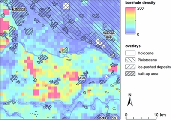
Fig. 4. Current data distribution in the study area, see Fig. 1 for geographical and geological reference. The Holocene floodplains are clearly better sampled than the Pleistocene terrains, which is largely because of the additional boreholes of Utrecht University used for GeoTOP modeling (see text for explanation). The size of the grid cells is 1 km.
Soft data
Besides working at ever-increasing resolutions, the extent to which interpolation routines were geologically constrained increased. Lithology and associated properties are geologically confined at various scales: from within lithostratigraphic units (which our Survey defines on the basis of macroscopically observable rock characteristics), down to their constituents (ranging from stratigraphic members to single facies units).
The more geological features are represented in the model, the more detailed and geologically appealing it will be, and the better it will presumably predict aggregate prospectivity. We currently achieve this by using available geological information deterministically, e.g. stratigraphic concepts and geological maps. In the Aggregates model this approach has not yet been used and all boreholes were interpolated within the 3D model space without considering their lithostratigraphical context, so the extent to which that model is realistic is primarily attributable to data density (and of course quality).
In the Delfstoffen Online model, interpolation was confined to the lithostratigraphic units of the Digital Geological model (DGM; Gunnink et al., Reference Gunnink, Maljers, Gessel, van, Menkovic and Hummelman2013). DGM is a 3D geological raster model consisting of a stack of grids representing the tops and bases of Quaternary and Neogene formations, based on a set of 16,500 high-quality, stratigraphically interpreted borehole descriptions. The Holocene, however, while divided into two formations in the study area, is represented by a single composite unit (Fig. 2).
A refined version of DGM, based on all available boreholes instead of the aforementioned subset, is used in the production of GeoTOP and additional detail was added. The Holocene composite unit in the study area was subdivided into its constituents: Echteld Fm (fluvial), Nieuwkoop Fm, Basisveen Bed and Hollandveen Mbr (see above). Within the Boxtel Fm, where possible, we mapped the Wierden Mbr (see above), Singraven Mbr (brooke facies) and Kootwijk Mbr (aeolian drift). Finally, fluvial Holocene channel belts, mapped by Berendsen & Stouthamer (Reference Berendsen and Stouthamer2001) and Cohen & Stouthamer (Reference Cohen and Stouthamer2012), were incorporated into the model as separate entities to further constrain interpolations. These channel belts are mapped at a scale of 1:100.000, the smaller ones being less wide than the grid resolution of 100 m. Mapping originally relied on the combination of augering and field geomorphology. Following the approach of Berendsen (Reference Berendsen2007), considerable improvements in mapping accuracy have been achieved by using Actueel Hoogtebestand Nederland (AHN). AHN is a national high-resolution elevation model based on airborne laser altimetry, which reveals channel belts as subtle elevations with respect to the more compactable floodplain fines.
The mapped outline of channel belts acts as a lateral boundary in the interpolation step of GeoTOP and is kept constant throughout the modelling process. The top and base of the channel belts are constructed using borehole data. The voxels within the channel belts are filled using only lithological information from boreholes within the channel belt, and the voxels outside this outline are filled using only boreholes outside the belt. In this way the generally better sampled floodplain fines do not ‘dilute’ the sandier channel belts, or vice versa.
Modelling techniques
Each of the three models was constructed with a different interpolation technique (Table 2), but the outputs were processed in the same way, i.e. by applying resource and exploitability criteria to individual voxel stacks down to certain desired depths. The same criteria were used to produce map output of total and exploitable resource amounts for all three models (Fig. 5). Linear kriging, i.e. ordinary kriging with a linear variogram, was used for the interpolation of the Aggregates model (van der Meulen et al., Reference van der Meulen, van Gessel and Veldkamp2005). As we were only interested in the estimated values, the slope of the variogram is not requested by the algorithm, therefore the only way to account for geological variability while using this technique is in setting the search neighbourhood, which determines to which distance samples will contribute to the estimation for a voxel. Punctual kriging was used for the Delfstoffen Online model, using a single search neighbourhood and variogram for the entire model space, i.e. the same ones irrespective of the DGM unit. A variogram describes the spatial distribution and structure of the samples: it weighs the contribution of samples within the search neighbourhood (in general, the closer the sample, the greater its weight).
Table 2. Overview of the model properties.

For modelling techniques see Goovaerts (Reference Goovaerts1997) and Chilès & Delfiner (Reference Chilès and Delfiner2012). The interpolations were performed in the commercially available software package Isatis® by Geovariances.
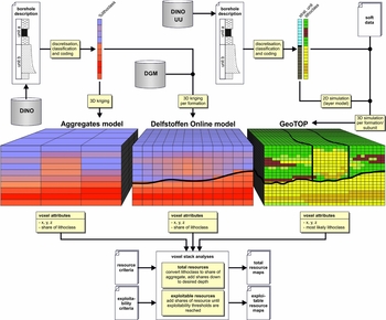
Fig. 5. Generalised workflows for the Aggregates, Delfstoffen Online and GeoTOP models. Resource criteria refer to Table 1. General principles are outlined in the text and details can be found in Table 2 (model parameters), van der Meulen et al. (Reference van der Meulen, van Gessel and Veldkamp2005, Reference van der Meulen, Maljers, van Gessel and Gruijters2007b) and Stafleu et al. (Reference Stafleu, Maljers, Gunnink, Menkovic and Busschers2011, Reference Stafleu, Maljers, Busschers, Gunnink, Schokker, Dambrink, Hummelman and Schijf2012).
For GeoTOP we transformed every description interval into an indicator, i.e. the discrete descriptor ‘lithoclass’ (Fig. 5). Sequential indicator simulation (SIS) was used for the interpolation step, using a search neighbourhood and variogram model per geological unit, resulting in voxels having a most likely lithoclass estimate. The final model product is averaged from 100 equiprobable simulations using the method described by Soares (Reference Soares1992; Stafleu et al., Reference Stafleu, Maljers, Gunnink, Menkovic and Busschers2011, Reference Stafleu, Maljers, Busschers, Gunnink, Schokker, Dambrink, Hummelman and Schijf2012). Note that the standard GeoTOP lithoclasses described by Stafleu et al. (Reference Stafleu, Maljers, Gunnink, Menkovic and Busschers2011) differ from the ones we use for aggregate resource assessments (Table 1), so a different GeoTOP variant was created for this particular application, using the standard workflow with adapted settings.
Resource maps are derived from voxel models by the analysis of vertical cell stacks. Total resource maps are generated by summing voxels which meet the selected resource criterion down to the desired exploration depth. Exploitable resource maps are generated by considering the thickness of an overburden or intercalation layer of clay and/or peat, discarding aggregates below such layers if set thickness thresholds are exceeded.
Results
Fig. 6 shows total and exploitable resources of coarse sand and gravel in the study area as predicted by the three models. The most obvious difference, apart from resolution as such, is the extent to which geological features are distinguishable, especially in the exploitability maps, which are most susceptible to geological variation. Only national-scale features appear in the Aggregates model, most notably the ice-pushed ridges, the Roer Valley Graben system and the general difference between Holocene and Pleistocene terrains in the northwest and southeast of the country, respectively (see Fig. 1 and van der Meulen et al., Reference van der Meulen, van Gessel and Veldkamp2005). The dimensions of these phenomena exceed those of the study area, where only the differences between the Rhine-Meuse Delta, the Utrechtse Heuvelrug ridge and the hinter-lying glacial basin in the northeast stand out. As proof of concept, the aggregate resource assessment based on the Aggregates model was only successful in predicting general areas of higher prospectivity, which correspond to concentrations of extraction sites. This assessment is clearly not suitable for site-scale assessments and was never used for that purpose.
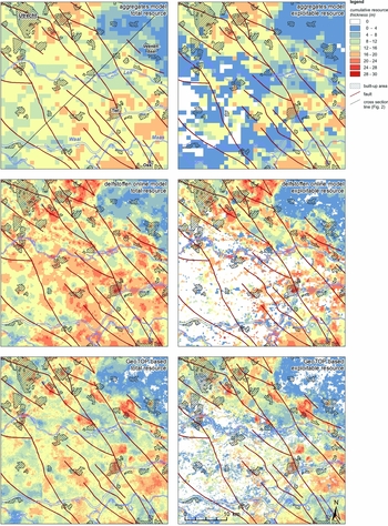
Fig. 6. Total (left column) and exploitable (right column) coarse aggregate resources in the study area down to 30 m below the surface, according to the Aggregates model (upper row), Delfstoffen Online model (middle row) and GeoTOP (lower row).
The assessment based on the Delfstoffen Online model retains these general features, and the exploitability map better reflects the heterogeneity of the delta plain. However, while the channel belts that mainly cause this heterogeneity are more or less identifiable, they are rather patchily represented. The same map derived from the GeoTOP model on the one hand shows more continuous channel belts, but on the other also a more heterogeneous pattern in between, in the flood basins, which is not or hardly present in Delfstoffen Online. Fig. 7 shows both effects in more detail, in a cross-section perpendicular to the belt of the river Linge, a minor Rhine distributary. In the Delfstoffen Online cross-section, floodplain and channel deposits are ‘mixed’ to the extent that the channel is not recognisable as an entity, neither in cross-section, nor on the map. In GeoTOP, however, the Linge channel belt is clearly represented, as is a smaller one to the north.

Fig. 7. Cross-section through the channel belt of the river Linge based on the Delfstoffen online model (upper panel) and on GeoTOP (lower panel). The upper panel shows the share of aggregate (blue, low percentages; red, high percentages); the lower panel shows the discrete lithoclasses. The reference datum for both cross-sections is NAP (Dutch Ordnance Datum). The extent to which the channel belt is resolved is also evident from the location maps, which show exploitable resource of coarse aggregate for both models. The colour scale used in the maps is as in Fig. 6; grey shading, channel belts (Berendsen & Stouthamer, Reference Berendsen and Stouthamer2000); black dots, boreholes in DINO; red dots, boreholes obtained from Utrecht University.
A second important difference is in the resource amounts: the maps in Fig. 6 derived from the Delfstoffen Online model are clearly ‘redder’, indicating higher resource amounts than those from the other two models. Fig. 8, a graph of bulk total and exploitable resource volumes in the study area, shows that Delfstoffen online contains some 20% more resource in comparison with the other two models. Fig. 8 also shows that the Delfstoffen Online predicts lower exploitability down to 30 m than the other two.

Fig. 8. Cumulative total (in orange) and exploitable (in green) coarse aggregate resources down to 10 and 30 m below the surface according to the Aggregates, Delfstoffen Online and GeoTOP models. For example, the Delfstoffen Online model predicts a total amount of 23 km3 down to 30 m below surface level, of which 13 km3 or 57% is exploitable.
Figs 9 to 11 show the dependency of total and exploitable resource estimates down to 30 m below the surface on grain-size category in Delfstoffen online and GeoTOP (as the Aggregates model did not have multiple grain-size categories), expressed in resource maps and resource volumes. The difference is primarily in the share of coarse aggregate in the total volume of all sand and gravel: the cumulative volume of all aggregates is the same and the medium category differs only slightly; exploitable resources vary proportionally but overall exploitability is higher for GeoTOP (Fig. 11). The integrity of the channel belt network, again, is even more visible in the upper panel of Fig. 10, which show the exploitability of all sand and gravel regardless of grain size: patchy for Delfstoffen Online versus more continuous channel belts in GeoTOP, alternating with more heterogeneous flood basins.

Fig. 9. Total resources of all sand and gravel (upper row), medium coarse aggregate (middle row) and coarse aggregate (lower row) down to 30 m below the surface, according to the Delfstoffen Online model (left column) and GeoTOP (right column).

Fig. 10. Exploitable resources of all sand and gravel (upper row), medium coarse aggregate (middle row) and coarse aggregate (lower row) down to 30 m below the surface, according to the Delfstoffen Online model (left column) and GeoTOP (right column).

Fig. 11. Cumulative total and exploitable aggregate resources in the study area in three grain-size categories down to 30 m below the surface, calculated from the Delfstoffen Online and GeoTOP models.
Discussion
Aggregate resource estimates provide a common ground for comparisons between three successive generations of voxel models produced by the Geological Survey of the Netherlands, which differ in terms of purpose, resolution and attribution. The different methods used for the three models share the general principle that the proportions of lithoclasses in the model output correspond to those in the input data. The boreholes used for resource characterisation were virtually the same, as the Utrecht University dataset primarily covered the top layer, i.e. the overburden. The observed differences in coarse aggregate resource amounts can therefore only arise from choices during the data preparation step. More specifically, two seemingly arbitrary choices made when mapping older sediment classifications to the grain-size categories we use for resource assessment purposes have affected the outcomes to a significant extent, at least for the coarsest resource category.
Delfstoffen Online predicts lower exploitability down to about 30 m than the Aggregates model, even though the models are similarly attributed and have the same vertical resolution. This means that, on average, exploitability thresholds are reached at shallower depths in Delfstoffen Online, which suggests that clay and peat are better confined to the overburden layer, just as can be expected from using DGM in the interpolation step.
GeoTOP predicts higher exploitability than Delfstoffen Online because better resolved features such as the channel belt network provide more ‘access’ to the underlying resource (as demonstrated in detail in Fig. 8). The similarity in total sand and gravel volumes in Delfstoffen Online suggests that the area was already well enough sampled without the extra Utrecht University boreholes to predict averaged subsurface properties. However, while these boreholes did not appear to add to averaged properties, they clearly enabled us to better capture the 3D geometry of the channel belts.
The answer to the question whether each next generation in voxel modelling was worth the investment, based on the present evaluation, is ‘yes’, for a simple reason. While we considered an area of 40 × 40 km, site pre-prospection is obviously done at much smaller scales; the largest Dutch aggregate pit has a surface area of about 4 km2. The Aggregates model was clearly unsuitable for that purpose. Delfstoffen Online was a major improvement, but its patchiness presents a problem. If, for example, the model would be consulted between two patches of high prospectivity that should actually have been connected, then the area could theoretically be discarded for wrong reasons. Hence, the extra geological constraints used in GeoTOP modelling improved the results in a way that is relevant to the application at hand. More obviously, additional data, which enable better characterisation of the flood basins, improved the output for similar reasons. More generally speaking, our progress in voxel modelling is expressed in a better prediction of subsurface properties. Average properties are about the same in all three models; variation and heterogeneity became better represented over time.
Conclusions
Progress made in our geomodelling efforts has largely been enabled by increasing computer power and project budget. This allowed us to deploy evermore elaborate modelling workflows, increasing the resolution at which we model, and including more geological data to better constrain the interpolations. The present paper essentially compares model realisations at three different scales. In a formal geodetic perspective it is not fair (or even correct) to compare the models as we did: at the same scale. The specific reason why GeoTOP is better than the previous models that it is the best fit for the purpose: it best approximates the desired scale for the application at hand.
In the future, the main delimiting factor for our geomodelling efforts will be data availability (van der Meulen et al., Reference van der Meulen, Doornenbal, Gunnink, Stafleu, Schokker, Vernes, van Geer, van Gessel, van Heteren, van Leeuwen, Bakker, Bogaard, Busschers, Griffioen, Gruijters, Kiden, Schroot, Simmelink, van Berkel, van der Krogt, Westerhoff and van Daalen2013). In that context, it is most relevant that the Geological Survey of the Netherlands is preparing for a new law on subsurface information in the Netherlands. Under this law, DINO will be upgraded to a key register for the subsurface, an official type of database in which the government uniquely stores data that is vital to its tasks. This upgrade is associated with a standardisation effort and the obligation of government bodies to feed and consult the register. This will raise the consistency and volume of subsurface data, and undoubtedly prove a sine qua non for further improvement of our subsurface models and all activities that use them, such as assessing aggregate resources.
There are two more general lessons to be learned from our analysis. The first is related to the management of geological information. Whilst the specifications, properties and outputs of the older models we assessed were retained, the modelling as such turned out not to be completely reproducible because this would require using vintage software as well as a ‘frozen’ excerpt of our database as it was at that time. Even though it did not present limitations to the present study, we recommend that special attention is paid to reproducibility, not only for systematically produced models such as GeoTOP, but also for one-off exercises conducted for proof of concept, contract research, etc. This will increase the reuse possibilities of geological information products in unanticipated situations (including the present study into modelling progress).
The second lesson is related to the fact that, while the highest-resolution model was best-suited for resource assessments, the oldest one has in fact not been invalidated (provided that it is used at the appropriate scale). The two orders of magnitude difference in investment between two basically useful models indicates that it is very important to thoroughly articulate the problem that is to be addressed by a subsurface modelling exercise.
Acknowledgements
The authors thank Dr Kevin J. Keogh and an anonymous reviewer for their reviews of this paper. Their suggestions helped us to significantly improve our manuscript.


