Introduction

Bed topography and ice thickness are essential characteristics of glaciers and ice sheets for many glaciological applications, but they remain difficult to measure remotely. This is especially true for ice-sheet coastal sectors and mountain glaciers, where the ice surface is significantly broken up, the ice substrate is near or at the melting point, and scattering and signal absorption are high. At present, bed elevation and ice thickness are mapped using airborne radar-sounding profilers, i.e. sounders that detect radar echoes from the bed directly beneath the aircraft carrier and convert these echoes into bed elevation, surface elevation and ice thickness (Reference GogineniGogineni and others, 2001). The radar-profiler mode (PM) data are then interpolated onto a regular grid using various methods, most commonly geostatistical techniques, such as kriging (e.g. Reference BamberBamber and others, 2013; Reference FretwellFretwell and others, 2013) or more sophisticated algorithms (e.g. Reference Herzfeld, Wallin, Leuschen and PlummerHerzfeld and others, 2011). The absolute precision of these gridded products is difficult to quantify in the absence of independent measurements of ice thickness. This is an issue for ice-sheet numerical models, which employ these data, especially in areas with few data and potentially large interpolation errors.

Russell Glacier is a land-terminating glacier in central-west Greenland, 20 km east of Kangerlussuaq near Søndre Strømfjord (67° N, 50°W), that has not changed significantly in recent years (Reference Pritchard, Arthern, Vaughan and EdwardsPritchard and others, 2009). In 2010 and 2011, NASA’s Operation IceBridge (OIB) conducted a dense radar survey (500 m track spacing) of Russell Glacier (Fig. 1), to evaluate our present-day mapping capability, evaluate the precision of the radar data (e.g. through crossover analysis), compare different techniques of bed mapping and evaluate their errors and potential impact on numerical ice flow models. Here we compare the results obtained using three methods: (1) a radar tomography (RT) processing of the radar data to produce a gridded map of bed elevation, (2) a method of ordinary kriging (KR) applied to radar-derived ice thickness data along the flight tracks to obtain a regular grid of ice thickness, and (3) a reconstruction of ice thickness on a regular grid using the principle of mass conservation (MC) applied to the radar-sounding derived thickness data combined with ice motion data from satellite radar interferometry within an optimization framework. The RT method is a novel, high-resolution processing technique, which requires a dense grid of flight tracks to produce a contiguous map of bed elevation over a large area. The second method is a standard method for producing ice thickness and bed elevation maps from radar profilers. The third method calculates ice thickness values on a triangle mesh and solves for the mass conservation using the finite-element method, while at the same time minimizing the departure of the results from the original radar-derived ice thickness data (Reference Morlighem, Rignot, Seroussi, Larour, Ben Dhia and AubryMorlighem and others, 2011). These methods are here compared over an exceptionally dense network of radar observations. This setting is ideal for evaluating errors in radar-derived ice thickness, bed elevation and flux divergence and for comparing the performance of various methods. Because this level of mapping is not practical over large areas, we also investigate the impact of reducing the number of tracks used to survey bed elevation and ice thickness to determine the configuration required to achieve a given precision in bed elevation and ice thickness mapping. We discuss the impacts of the results on ice-sheet modeling and conclude with recommendations for bed elevation mapping of glaciers and ice sheets.

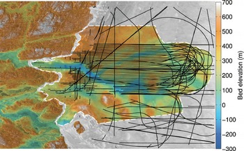
Fig. 1. Bed topography of Russell Glacier inferred using the mass continuity (MC) method at 400 m resolution, calculated as surface elevation minus ice thickness. The dashed white line defines the limits of the model domain. NASA OIB flight tracks are indicated as black solid lines. Surface elevation is from the Greenland Ice Mapping Project (personal communication from I. Howat, 2012), including over ice-free zone. Note the agreement between ice-free and ice-covered elevations.

Data and Methods

Ice velocity data

We measure ice velocity using a combination of Advanced Land Observing Satellite (ALOS) Phased Array-type L-band Synthetic Aperture Radar (PALSAR), RADARSAT-1 and Envisat Advanced SAR (ASAR) speckle-tracking data (Reference Rignot and MouginotRignot and Mouginot, 2012). Data resolution is 350 m, precision in speed is 10 m a⁻¹ and in direction is 1° (Fig. 2). The glacier speed is ∼150 m a⁻¹ at the equilibrium-line altitude, and decreases to a few meters per year at the ice margin. The velocity map reveals that Russell Glacier shares a common source with two other glaciers: Isunguata Sermia to the north, which flows at a comparable speed, and a glacier which we identify as South Russell to the south, which flows at ∼380 m a⁻¹.

Fig. 2. Observed ice surface motion derived from satellite radar interferometry data using speckle tracking (Reference Rignot and MouginotRignot and Mouginot, 2012) overlaid on a backscatter image from Envisat ASAR 2009.

Radar tomography (RT)

We apply RT processing to a portion of the OIB data where the flight pattern is most regular and provides a nearly contiguous coverage of the bed. The processed area, located in the northeastern sector of the survey grid, is 15 km × 30 km in size (Fig. 3e). Unlike conventional radar-sounding profilers, where echoes from the left and right sides are not resolvable, RT relies on multiple antennas and multiple receivers in the across-track direction to differentiate the echoes (Reference Paden, Akins, Dunson, Allen and GogineniPaden and others, 2010; Reference Wu, Jezek, Rodriguez, Gogineni, Rodriguez-Morales and FreemanWu and others, 2011). RT resolves the bottom signal arrival angle and strength, which are then used to derive the bed topography. The measurable swath width depends on the signal-to-noise ratio (SNR), which can vary strongly depending on basal roughness and ice absorption rates. RT produces here fine-resolution (20 m spacing) estimates of bed elevation over a swath width of 1600 m, with a standard noise of 10 m (Reference Wu, Jezek, Rodriguez, Gogineni, Rodriguez-Morales and FreemanWu and others, 2011). We use this map as one of our reference datasets to evaluate the performance of other techniques since it is the only technique capable of dealing with off-nadir errors, which have recently been shown to be significant in the conventional PM radar processing (Reference Wu, Jezek, Rodriguez, Gogineni, Rodriguez-Morales and FreemanWu and others, 2011).

Fig. 3. Bed topography of Russell Glacier with respect to mean sea level, with elevation contours at 50, 200, 350 and 500 m, from (a) Reference Bamber, Layberry and GogineniBamber and others (2001), (b) Reference BamberBamber and others (2013), (c) mass continuity (MC), (d) ordinary kriging (KR) and (e) radar tomography (RT); (f) zoom of (e).

Ordinary kriging (KR)

Kriging combines nearby observations to predict bed elevation (or ice thickness) at other locations (Deutsch and Journel, 1997). This technique has been used extensively for mapping surface elevation, ice thickness (e.g. Reference Griggs and BamberGriggs and Bamber, 2011) and bed elevation (e.g. Reference BamberBamber and others, 2013; Reference FretwellFretwell and others, 2013). Ice thickness, H, at a given location (x, y) is assumed to be a linear combination of a subset of observations, H_i :

(1)

where λ_i (x, y) are the kriging weights and is the subset of nearby observations. In our application, includes the closest 200 measurements within a radius of 50 km around (x, y). We employ a particular type of kriging named ordinary kriging, which is a very common type of kriging (Deutsch and Journel, 1997). Ordinary kriging assumes a constant but unknown mean and the kriging weights fulfill the unbiasedness condition:

(2)

The weights are calculated to minimize the variance of the estimation error, assuming that ice thickness is a random process for which we estimate the covariance structure. We derive the covariance from a semivariogram assuming an exponential model. We use a nugget effect of 50 m to account for measurement errors, and find a best fit between model and observations for a range of 4.3 km and a sill of 58 km. The data are interpolated on a regular grid at 500 m spacing. Bed elevation is deduced by subtracting H from the digital elevation model (DEM) of the Greenland Ice Mapping Project (GIMP), that combines ASTER (Advanced Space-borne Thermal Emission and Reflection Radiometer), SPOT-5 (Système Pour l’Observation de la Terre) and AVHRR (Advanced Very High Resolution Radiometer) photoclinometry (personal communication from I. Howat, 2012).

Mass conservation (MC)

The mass conservation (MC) method combines ice thickness data with ice velocity to infer a spatially consistent map of ice thickness that fulfills the continuity equation. This method was originally introduced by Reference RasmussenRasmussen (1988) and applied to Columbia Glacier, Alaska, USA.

The MC method relies on the depth-integrated continuity equation. Ice thickness, H, must satisfy the following equation:

(3)

where is the depth-averaged ice velocity, and is the apparent mass balance, i.e. the sum of surface mass balance, basal melting and thinning rate (Reference Morlighem, Rignot, Seroussi, Larour, Ben Dhia and AubryMorlighem and others, 2011). Ω is the model domain and Γ₋ the inflow boundary, where measurements of ice thickness, H _obs, are required and imposed. The bed elevation is deduced by subtracting H from a surface elevation dataset.

This standard approach yields products that may deviate significantly from the measurements due to errors in the input data (Reference Morlighem, Rignot, Seroussi, Larour, Ben Dhia and AubryMorlighem and others, 2011). The only ice thickness data that constrain the computation of ice thickness in this method are along the inflow boundary Γ₋.

Here we employ an improved method, which uses all available thickness measurements within the model domain instead of along the boundary only, and the method takes into account errors in the input data, i.e. ice velocity, apparent mass balance, and ice thickness. We formulate an optimization problem by defining the following objective function:

(4)

where T ∊ Ω are the flight tracks where ice thickness, H _obs, is measured, and γ is a regularization parameter. The first term of Eqn (4) represents the mismatch between modeled and measured thickness. The second term is a regularizing constraint, which penalizes wiggles in ice thickness. The addition of regularization is essential to infer smooth spatial variations in ice thickness. A large value of γ yields a smoother thickness map that deviates more from observations, whereas a small value of γ produces a good fit with observations but with strong gradients near flight tracks. γ is here kept constant for the entire domain, but it could be spatially variable to better model regions of known high thickness gradients; this aspect ought to be investigated in more detail in the future. We select γ = 10⁵ using an L-curve analysis (Reference Hansen and JohnstonHansen, 2001), which optimizes the trade-off between the two terms that should be controlled.

The depth-averaged ice velocity, , is not calculated from an ice-sheet model but is assumed to be equal to the surface velocity derived from satellite radar interferometry data (Reference Rignot and MouginotRignot and Mouginot, 2012). The absence of a model is justified for two reasons: (1) Relying on an ice-sheet model would introduce a circularity in the problem since the modeled velocity depends on ice thickness, and MC thickness is constrained by ice velocity (Eqn (3)). (2) Because the MC method relies on a transport equation (Eqn (3)), the solution for H is sensitive to errors in flow direction. Even with the additional support of inversion methods (e.g. Reference MacAyealMacAyeal, 1993; Reference Morlighem, Rignot, Seroussi, Larour, Ben Dhia and AubryMorlighem and others, 2010), modeled flow directions are generally less precise than direct measurements, so using a model would actually increase the misfit between observations and calculated thicknesses.

The tolerance interval for depth-averaged velocities, , is derived from measurement errors and from the assumption that surface velocities are uniformly representative of column velocities, which is a reasonable assumption for fast-flowing glaciers but may not be reasonable for slow-moving ice (e.g. around domes or ice divides). We checked this assumption with a higher-order ice-sheet model (Reference BlatterBlatter, 1995; Reference PattynPattyn, 2003). The results show that surface speeds are <3% larger in magnitude than depth-averaged speeds over the entire domain Ω. To allow enough flexibility in the optimization process, we use a tolerance on ice velocity that is larger than the nominal error. We use an asymmetric error for : the upper bound is 15 m a⁻¹ above the observed surface velocity; the lower bound is 5% smaller than the observed surface velocity.

For the apparent mass balance, we assume that the rates of basal melting and surface lowering of Russell Glacier are negligible compared to its average surface mass balance. Surface mass balance from a regional atmospheric climate model RACMO2 (Reference EttemaEttema and others, 2009) ranges from −250 cm a⁻¹ at the ice margin to −50 cm a⁻¹ in the interior of the study domain for the time period 1961–90 (Reference EttemaEttema and others, 2009). The tolerance interval for the apparent mass balance accounts for errors in basal melting rates, surface mass balance and ice-thinning rates. Errors in surface mass balance are at the 10% level (∼20 cm a⁻¹). Errors in melting rates are small (<1 cm a⁻¹). Satellite laser altimetry (Ice, Cloud and land Elevation Satellite (ICESat) and Airborne Topographic Mapper (ATM); personal communication from B. Csatho, 2012) shows that thinning rates reach 80 cm a⁻¹ in this region. We therefore consider a tolerance interval of ±1 m a⁻¹ for apparent mass balance.

Here MC is more sensitive to errors in velocity directions than errors in apparent mass balance. The ice velocity controls almost entirely the mass flux at a given location of the model domain compared to the apparent mass balance, which is significantly smaller than the mass flux from the ice coming upstream.

The spatial resolution of MC is constrained by the spatial resolution of the ice velocity data, here 350 m. We use a finite-element mesh of 25 000 elements ∼400 m in size. We stop the optimization procedure when the objective function, , reaches a value that corresponds to a misfit of <30 m between modeled and measured thicknesses along the flight tracks T, which is consistent with the analysis of crossover errors quoted earlier.

Results

The bed topography derived from the MC method ranges from +700 m for the highest points to 300 m below sea level in troughs (Fig. 1). Bed troughs strongly coincide with areas of fast flow in Figure 2, i.e. ice is channelized along topographic valleys. Conversely, ice flow is slower and thinner on the surrounding topographic ridges and peaks. These features are consistent in location, orientation, size and elevation with valleys and ridges present in the digital topography of ice-free areas, which is available at a higher resolution (90 m) with a higher vertical precision (±10 m). The two independent data sources form an almost seamless reconstruction of the bed across the ice margin, except for a band ∼500 m wide, where the MC method does not apply because the ice velocity drops to values that are too low (<20 m a⁻¹)to be applicable. The remarkable consistency of the two maps provides an independent evaluation of the quality of the MC results.

The standard error in bed elevation from the MC method is 36 m with respect to RT (Table 1) and 34 m with respect to PM. The KR bed topography yields similar results, when compared to both RT and PM. In the bed elevation from Reference Bamber, Layberry and GogineniBamber and others (2001), which is commonly used in ice-sheet models, most spatial features present in the KR and MC maps are absent (Fig. 3a). The updated version of this dataset (Reference BamberBamber and others, 2013, fig. 3b) is more consistent with OIB measurements, but errors in bed topography still exceed 50 m when compared to RT and PM.

Table 1. Comparison of bed elevation obtained using ordinary kriging (KR) and the mass continuity (MC) methods versus the radar tomography (RT) results over a limited domain and versus the original measurements in profiling mode (PM) over the entire domain, for different flight-track spacings: inflow boundary only, 5 km, 2.5 km and 500 m. For reference, the standard error (σ_H ) between PM and RT is 46 m (right column). The bottom rows give the standard error in flux divergence (σ _FD) over the entire model domain, and the maximum flux divergence error (ΔFD_max)

The RT bed elevation map (Fig. 3e and f) is of higher vertical precision and higher resolution than the other maps but it is limited in spatial extent because the ensemble of overlapping RT flight tracks is limited in size and also because the RT results have data gaps in the deeper parts of the troughs. These data gaps are associated with the SNR of the data that exceeds a given threshold selected during RT processing. We choose a conservative threshold here to minimize errors so that the method yields a product relatively free of artifacts, which we use in turn as a reference. With a more aggressive selection of the threshold, the processing would recover additional points in the trough, at the expense of data noise.

Comparing RT with other methods along profile A–B (Fig. 4), we observe significant differences between PM and RT, which we attribute to errors from off-nadir reflections in the PM products. The MC and KR methods yield smoother, lower-resolution results.

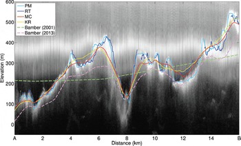
Fig. 4. Comparison of bed elevations along profile A–B in Figure 3e, overlaid on a radar echogram (frame 02_20110413_03_024). The bed elevations of mass continuity (MC) and ordinary kriging (KR) are smoother than the profile-model processing (PM) and radar tomography (RT) due to their resolution of 400 m.

The flux divergence is another important quantity to examine during the mapping of ice thickness because ice thickness data are typically combined with ice motion data in ice-sheet models to calculate the ice thickening/thinning rate. The mass conservation equation (Eqn (3)) indicates that the flux divergence should be equal to the apparent mass balance when the glacier is in steady state. The flux divergence should therefore be smaller than ∼1 m a⁻¹. Large values of the initial flux divergence (several m a⁻¹) in a numerical ice-sheet model would force the model to redistribute mass in order to reconcile topography and ice motion, thereby changing the glacier surface topography, and converge to a steady state that may differ significantly from the initial condition (Reference SeroussiSeroussi and others, 2011). When combined with ice velocity, the KR map yields errors in flux divergence up to 360 m a⁻¹, which is large. Flux divergence errors for Reference Bamber, Layberry and GogineniBamber and others’ (2001, Reference Bamber2013) maps exceed 2000 m a⁻¹, probably because of their lower spatial resolution (5 km and 1 km respectively). In contrast, MC yields flux divergence errors smaller than 1 m a⁻¹, which is the selected tolerance interval for the apparent mass balance.

In a second set of experiments, we reduce the number of flight lines used in the mapping to determine how the performance of KR and MC methods evolves when the track spacing increases. We first consider only the measurements that are along the model inflow boundary (Fig. 5c), and run the two methods of KR and MC, using the same numerical settings. The KR method produces a nearly flat bed with no valleys (Fig. 5a), and large errors (Table 1), whereas the MC method yields correct spatial features (Fig. 5b), with a standard error of 110 m. We then use only one-tenth of the flight lines, hence simulating a track spacing of ∼5 km (Fig. 5f), and finally one-fifth of the flight lines, for a track spacing of 2.5 km (Fig. 5i). The results are shown in Figure 5d and g for KR, and Figure 5e and h for MC. Both maps are closer to the observations, and the troughs are more visible as the track spacing decreases. The bottom row of Figure 5 shows the maps obtained when all flight tracks are used, which corresponds to a track spacing of ∼500 m (Fig. 5l).

Fig. 5. Ice thickness of Russell Glacier for different sets of radar observations. The first column (a, d, g, j) corresponds to KR maps of ice thickness; the second column (b, e, h, k) corresponds to MC maps; and the last column (c, f, i, l) shows the corresponding radar tracks (PM) used as observational constraints in each row. In the first row (a–c), we only use measured ice thickness at the model inflow boundary. In the next rows, we use, respectively, one-tenth of, one-fifth of and all radar tracks, corresponding to track spacings of, respectively, 5 km, 2.5 km and 500 m.

When the track spacing increases from 500 m to 5 km, i.e. by a factor 10, the error in MC increases from 35 m to 65 m. The error for KR increases from 35 m to 80 m. The error in the KR method degrades more rapidly when the track spacing is increased than for the MC method, but the error in both methods does not decrease linearly with the track spacing. For flux divergence, with only one track at the inflow boundary, the KR error exceeds 900 m a⁻¹. At 5 km and 2.5 km spacing, the error is still large. At 500 m spacing, i.e. when all tracks are employed, the error drops to 360 m a⁻¹, which is still too large for direct application of ice-sheet models. This problem does not occur with MC, which, by design, provides errors in flux divergence smaller than 1 m a⁻¹ for all experiments.

The estimated maximum potential error in MC bed elevation is shown in Figure 6. The error is low along flight tracks, where the results are constrained to match the input data, and it increases along flow. Maximum errors occur between flight tracks, as expected. The error increases as the track spacing increases. Errors are <50 m over most of the model domain, but exceed 100 m on the sides of the domain where few measurements are available and ice speed is low.

Fig. 6. Estimated maximum potential error in ice thickness derived from the MC method

Discussion

The bed topography of Russell Glacier is more complex than anticipated given the relatively smooth nature of its surface elevation and the absence of major spatial variations in speed. The results, however, reveal that the flow pattern of the ice and the shape of the bed are strongly related. Ice is preferentially channelized along deeply carved, narrow valleys, which in this case are below sea level. These channels are likely to result from repeated glacial erosion over glacial cycles (Reference Cook and SwiftCook and Swift, 2012). When the track spacing is 500 m, KR and MC both yield products with low standard error, but MC maintains much lower errors in flux divergence. At higher track spacing, KR yields smoother products that do not preserve continuous features with preferential orientation due to its isotropic nature, hence the presence of bed channels is less well elucidated than with the MC method and artifacts in elevation are introduced along the bed channels.

Reference Durand, Gagliardini, Favier, Zwinger and Le MeurDurand and others (2011) suggest that small-scale bed topography features of the order of 1 km in size significantly affect grounding line retreat of tidewater glaciers, and hence recommend digital maps of bed topography at a spatial resolution better than 1 km. Our analysis suggests that a precision of 50 m may be difficult to achieve with the KR method, but possible with the MC method. This result is of practical importance because it is difficult and costly to fly large areas at a 500 m track spacing. In contrast, a 2.5 km track spacing along the coastline has already been achieved along most of central west and northwest Greenland in 2011 and 2012.

Our estimated maximum error in bed elevation for the MC method is conservative because most of the OIB tracks flown on Russell Glacier are oriented in the direction of flow, which is the least favorable configuration for constraining mass transport. A more favorable flight pattern would be to orient flight tracks perpendicular to the flow direction because this constrains input and output mass fluxes better and minimizes the impact of errors in flow direction. With a more optimal configuration of flight tracks, the MC method should provide estimates of bed elevation – and ice thickness – with a precision of 50 m or better at 400 m resolution using a flight-track spacing of only 5 km according to the results of our study.

For higher-resolution mapping, i.e. 10 m spacing or similar to the RT method, higher-resolution ice velocity products are needed, which are achievable, for instance, using TERRASAR-X data (higher spatial resolution). Velocity mapping may also be improved by using the interferometric phase instead of speckle tracking (Reference Joughin, Smith and AbdalatiJoughin and others, 2010). Higher-precision products derived from the interferometric phase would make it practical to extend the MC method beyond the range of fast-flow areas. At present, the MC method is best applied to fast-flow areas surveyed with a track spacing of ∼5 km or better. This is also the portion of Greenland most relevant to high-resolution ice-sheet models projecting the evolution of the ice sheets into the coming decades to centuries.

Conclusion

The detailed study of the bed topography beneath Russell Glacier reveals that radar profilers (PM) yield errors in bed elevation four times larger than commonly thought. Furthermore, the traditional method of KR, with track spacings in the km range, yields products that do not capture important spatial features well if the track spacing exceeds ∼1 km and yield large errors in flux divergence when combined with ice motion data that are untenable for ice-sheet models. The reconstruction of bed topography using a combination of radar data and ice motion data offers significant advantages along coastal sectors. No model assumption is necessary other than neglecting internal shear. Areas where this assumption may be called into question are mostly slow-moving (speed less than ∼50 m a⁻¹). In the case of Russell Glacier, a land-terminating glacier in central-west Greenland, the application of the MC method reveals topographic features that are intimately responsible for the flow structure of the ice toward the ice margin. These features are robust, and consistent with spatial structures found on adjacent ice-free areas. The application of the MC method to the entire ice-sheet periphery therefore promises to be transformative of our knowledge of basal topography beneath glacier ice, which is, in turn, critical for the numerical modeling of the evolution of glaciers and ice sheets.