


MOTIVATION
The tree-ring section of the radiocarbon (14C) calibration curve is overwhelmingly based on measurements made by decay counting in the 1980s and 1990s (all but 56 of the 4314 measurements on tree rings included in IntCal13 were made in this way). At that time, 14C measurements performed by accelerator mass spectrometry (AMS) were not considered of comparable precision to results produced by decay counting (Schmidt et al. Reference Schmidt, Balsley and Leach1987; Fifield Reference Fifield2000), in which precision below 2‰ on modern samples was (and still is) possible (Stuiver Reference Stuiver1978; Stuiver Reference Stuiver1982; Stuiver and Becker Reference Stuiver and Becker1986; Hogg et al. Reference Hogg, Palmer, Boswijk and Turney2011).
Today, most 14C measurements are made by AMS, largely because much less sample material is required. At least several grams of wood were required for a high-precision measurement with decay counting, but only a few milligrams are required for AMS. While in principle modern AMS systems are capable of measuring at precisions of less than 2‰ on modern samples, it is still an open question if this precision and accuracy can be reached on a routine basis when much smaller samples are processed.
This single tree-ring intercomparison originated as a small experiment to systematically test the reproducibility of AMS measurements on wood samples following discussions at the IntCal meeting in Belfast in 2016. While eight laboratories initially planned to join the exercise, 16 laboratories ultimately took part.
The goal of the exercise was to test the precision and accuracy of the participating laboratories by analyzing and comparing a large number of replicated samples. Three sets of 21 consecutive single tree-ring samples from different time intervals, when no strong changes in 14C concentrations are expected, were used. The high replication should also allow for a meaningful statistical treatment of the results in order to reliably detect any laboratory biases.
The objective of this study was not planned to replace the successful series of international 14C intercomparison exercises (Rozanski et al. Reference Rozanski, Stichler, Gonfiantini, Scott, Beukens, Kromer and van der Plicht1992; Scott Reference Scott2003), in which all 14C laboratories are invited to assess their performance on individual samples and a consensus value is derived enabling the samples to subsequently be used as reference materials. A recent study has re-evaluated all AMS measurements on dendrochronologically dated wood samples (which were typically block samples of 20–40 rings) within these previous intercomparisons (Scott et al. Reference Scott, Cook, Naysmith and Staff2019). The precision (range of median errors) identified in that study was between 24 to 60 yr for individual measurements on samples with ages between 5000 BP and modern, which is nearly double that of measurements on wood of equivalent age included in IntCal13 (typically between 15 and 30 yr).
Here, our goal was to perform an intercomparison in which high-precision measurements were requested for the specific purpose of testing laboratory performance as part of constructing an accurate, new, annually resolved calibration curve.
SAMPLES AND ANALYSIS
Tree-Ring Samples
Three trees from different time periods within the Holocene were selected for this intercomparison. As the aim of the exercise was to test the laboratories systematically for their ability to produce accurate, high-precision 14C measurements, 21 continuous single tree-ring samples were prepared for each time period. Each 21-yr block was deliberately selected from a part of the calibration curve where atmospheric 14C varied little (i.e. from a plateau), as this provides a more powerful test of accuracy. The sample size of the raw wood supplied was deliberately limited to typically 30–50 mg. Samples contained earlywood and latewood. Dendrochronological information is given in the supplementary material.
All laboratories obtained 21 contiguous tree-ring samples for the years AD 1730 –1750 (Series H, 220–200 cal BP (AD 1950); Table 2), and AD 280–300 (Series A, 1670–1650 cal BP). For the years 5701–5681 BC (Series R, 7650–7630 cal BP) there was only sufficient material for 9 laboratories, owing to the fact that the exercise was originally planned for 8 laboratories. All laboratories were also supplied with two wood samples containing no detectable 14C that could be employed as a processing blank (brown coal from Reichwalde, Germany and an Oxygen Isotope Stage 5 kauri from New Zealand). While all laboratories processed wood blanks, three laboratories did not use either the supplied lignite or Stage 5 kauri.
Sample Preparation
All laboratories applied a pretreatment with acid and base followed by bleaching. About half of the laboratories started with an overnight base soak (Němec et al. Reference Němec, Wacker, Hajdas and Gäggeler2010) and one laboratory applied a solvent extraction by Soxhlet (Hoper et al. Reference Hoper, McCormac, Hogg, Higham and Head1998) as a first step. One third of the laboratories applied an additional α-cellulose step after bleaching (Hoper et al. Reference Hoper, McCormac, Hogg, Higham and Head1998).
Oxalic Acid 2 (OX2, NIST SRM 4990C) was the most common material used for standard normalization. One laboratory used only Oxalic Acid 1 (OX1, NIST SRM 4990B), while some laboratories used OX1 in addition to OX2.
Radiocarbon Analysis
Instrumentation and Data Reduction
Eight laboratories used a sub-1MV system (5 Micadas 0.2 MV, 3 NEC 0.5 MV) employing the 1+-charge state, while 2 laboratories used a 1 MV (HVEE, 2+-charge state) and 5 used a larger accelerator (3 MV or 5 MV from NEC or HVEE, ≥3+-charge state).
All laboratories using an ETH/Ionplus Micadas system, used the BATS program (Wacker et al. Reference Wacker, Christl and Synal2010) for data evaluation. The NEC ABC-software was also used frequently, sometimes in combination with the Data Fudger from the Lawrence Livermore AMS laboratory. About 1/3 of all laboratories use their own tools for data reduction (Donahue et al. Reference Donahue, Linick and Jull1990; Burr et al. Reference Burr, Donahue, Tang, Beck, McHargue, Biddulph, Cruz and Jull2007), either through coding their own programs or using Excel spreadsheets.
Replication of Data
Typically, each laboratory undertook one measurement per sample. Only one laboratory (Lab-2) systematically undertook duplicate measurements on each annual ring from the outset. A few laboratories repeated either specific series or some samples to test their internal variability. All repeats were performed on the same cellulose extraction with the exception of 4 rings of series R and A for Lab-2, for which the cellulose extraction was performed twice. Lab-9 always combined two consecutive tree rings so that enough material was available to survive the more rigorous α-cellulose treatment.
One laboratory (Lab-6) decided to retract their data for series H due to possible detector instabilities that became obvious after initial submission. Laboratory 14 submitted two independent measurement series of which only the second has been evaluated and is reported here (on the suggestion of the laboratory). Because of memory effects from a dirty ion source, the blank was 4-times higher than expected in a first run and consequently a second run was performed with a clean source. Interestingly, the dirty ion source resulted in 14C ages that are consistently 20 yr older.
Ultimately, more than 950 measurements were performed in total (H-series: 396, A-series: 353, R-series 203). Each ring was measured between 10 (R-series) and 20 times (H-series).
Blank Correction
Ten laboratories reported on blanks used for their data reduction. Most laboratories (8) relied only on full processing blanks, while one laboratory used both combustion and processing blanks, and one only used combustion blanks. The average blank used for the correction was F14C = 0.0019 (scatter: 0.0005). No consistent information was obtained about the estimated reproducibility of the blanks by individual laboratories but would be advantageous when sample ages are closer to the background (>10,000 BP).
Uncertainties by Laboratory
The laboratories followed very different approaches for estimating uncertainties. While many laboratories calculate their uncertainties on the larger of the counting statistic uncertainty or the internal variability of a sample measurement (variability of submeasurements of a single sample over time), other laboratories base their calculations on counting statistics where they add, in quadrature, an additional uncertainty (of typically 1–1.5‰), before adding an uncertainty for standard normalization and blank correction. While the first approach results in a relatively large variation in uncertainty, even within the same set of measurements (see also min and max uncertainties in Table 1), the latter provides less-variable uncertainties.
Table 1 The arithmetic means with its uncertainty and the median for all tree rings of the three series is given.

Statistical Analysis
In a first step, the error weighted mean for replicate measurements by an individual laboratory on each annual ring was calculated, assuming a systematic uncertainty of 1‰ from sample preparation (Sookdeo et al. Reference Sookdeo, Kromer, Buentgen, Friedrich, Friedrich, Helle, Pauly, Nievergelt, Reinig, Treydte, Synal and Wacker2019 in this issue) that is already included in the uncertainties given by the laboratories. The arithmetic mean ( ${\overline x_{ring}}$) and the median for each ring was determined, including the results of all 16 laboratories (AL). The mean is considered to be the consensus value for the individual tree-ring samples with the error estimated from the variance within the set of results. Thus, this error does not take account of the individual errors quoted by the laboratories. Statistical tests were typically performed on single measurements from specified laboratories against the consensus values (AL).
The distribution of a selection of laboratories (SL), which showed both (a) average uncertainties given by the laboratory of less than 20 yr on series H and A and (b) least variable offsets from the mean (Lab-1, 2, 5, 7, 8, 9, 14, 15–see also Discussion), was additionally compared to the distribution of AL. The offset (offlab) is the mean deviation of all n measurements of a laboratory ( ${x_{ring}}_i$) to the mean (${\overline x_{ring}}$):
 $$off_{lab} = \sum \limits_{ring,i}^n {{({{\overline x}_{ring}} - {x_{rin{g_i}}})} \over n}$$
The mean uncertainties produced by the laboratories were independently estimated for each series by comparing the measurements of a laboratory with the consensus values of all laboratories after subtraction of the laboratory offset:
 $${\sigma _{la{b_{series}}}} = \sqrt { {\sum \limits_{ring,i}^n {{{{({{\overline x}_{ring}} - ({x_{rin{g_i}}} - of{f_{lab}}))}^2}} \over n}}} $$
 The errors given by a laboratory ( $un{c_{rin{g_i}}}$) are finally compared with the observed deviations of the ring arithmetic mean value adjusted for the laboratory offset:
 $$\chi _{re{d_{la{b_{series}}}}}^2 = {{\sum \limits^n_{ring,i} {{{{({{\overline x}_{ring}} - ({x_{rin{g_i}}} - of{f_{lab}}))}^2}} \over {{un{c_{rin{g_i}}}}}^2}} \over n}$$
RESULTS AND DISCUSSION
Sample Mean and Comparison with IntCal13
The median and the arithmetic mean agree well with each other (Table 1), indicating a symmetrical distribution of data from all laboratories.
The mean, as well as the median, of all individual tree-ring measurements was calculated and compared with IntCal13, as shown with box plots in Figure 1. Series H is significantly older than the IntCal13 data. The offset is on average 16 ± 4 14C yr (in the following simply given as years), although this offset varies over the 21 yr supplied. While the mean offset of series A is –2 ± 6 yr, in good agreement with IntCal13, the offset of series R is 23 ± 8 yr, which is again statistically significant. We should note however, that IntCal13 is based on just a few decadal measurements in these time periods and consequently, offsets to IntCal13 cannot be determined as precisely. It may show that the interpolation between those few measured samples calculated for IntCal13 (IntCal13 provides data points for every 5th year) does not reflect the actual pattern of atmospheric 14C closely.

Figure 1 Box plot of the measurements of all laboratories for the individual series and the arithmetic means (black, gray) compared with IntCal13. The red data points are outside 1.5-times the interquartile range (indicated by min/max). (Please see electronic version for color figures.)
Laboratory Offsets
For each series, the mean laboratory offset relative to the overall mean and median is given in Table 2. As expected from the good agreement of the median and the mean, the offsets relative to the mean and median are all very similar. As a rule of thumb, deviations of less than 10 yr are acceptable within 2 σ, due to counting statistics and systematic effects of standard normalization. While about half of the laboratories seem to be consistently within ±10 yr (Labs-1, 2, 5, 7, 8, 9, 14, and 15), three laboratories have offsets of 10–20 yr (Labs-11, 13, 16), while other laboratories show larger and at the same time more variable offsets of up to 20–30 yr (Labs-3, 4, 6, 10, and 12). Over all, the measured offsets seem to be comparable to those observed on high-precision measurements (IntCal98) in the 1990s by decay counting (Stuiver et al. Reference Stuiver, Reimer, Bard, Beck, Burr, Hughen, Kromer, McCormac, van der Plicht and Spurk1998), in which laboratory offsets, primarily on measurements on decadal samples, were typically between 10 and 20 yr. However, today many more laboratories are able to produce data comparable to what was available in the 1990s. If only the 8 laboratories with the most consistent datasets (SL) are considered, a better constrained consensus value can be calculated.
Table 2 The performance of the laboratories relative to the mean and the median is given. Offsets and uncertainties are given in 14C yr (BP). The independently estimated uncertainty is calculated from the offset corrected deviations from the mean respectively the median. The χ2red is calculated from the estimated uncertainties relative to the quoted uncertainties.

Laboratory offsets seem to be distributed symmetrically, with large deviations to both younger and older ages. Laboratories with large offsets seem to be either consistently younger or consistently older for all series, pointing towards intrinsic systematic causes for the offsets. This observation needs to be investigated further by the laboratories concerned, as no obvious correlation is observed between these offsets and the information supplied about pretreatment protocols, blank subtraction, and standard normalization.
Estimation of Uncertainties
In order to better understand the accuracy of single measurements, their relative deviations from their corresponding mean are plotted as a histogram in Figure 2. The distribution is Gaussian-like in shape, and has a spread of about 21 yr for series H and A. This is clearly larger than the median of 17.5 yr for the quoted uncertainties. A reduced chi-square-test, comparing the deviations of the individual laboratories to the mean with their quoted uncertainties, shows that there is evidence of over-dispersion in comparison to what would be expected given the quoted uncertainties (χ2red≥1.6). This indicates that some laboratories are underestimating their uncertainties.
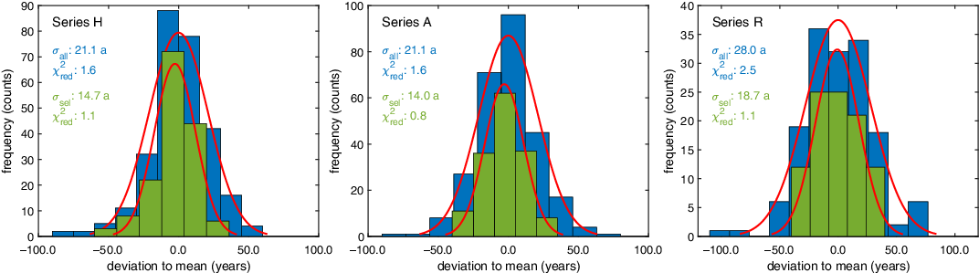
Figure 2 Distributions of deviations of all measurements of all laboratories (blue) and a selection of laboratories (green) around the means of the individual series. Positive deviations correspond to older ages. (Please see electronic version for color figures.)
In contrast, the selection of laboratories (SL) with the smallest and least variable offsets show significantly narrower distributions (σSL) for all series. The quoted uncertainties provided by these laboratories are also consistent with the observed deviations (although we are still comparing with the consensus value calculated from all of the data). This is indicated in Figure 2, with χ2red values for these laboratories of ~1.0 for all series.
The distributions of the SL show that AMS measurements from different laboratories can reproduce well within 2‰ (16 yr) for modern samples. The distribution is comparable to the one obtained for single-year data produced by a single laboratory at the University of Washington (QL) in the 1980s with high-precision gas proportional counting measurements (σQL=14.4) (Stuiver et al. Reference Stuiver, Reimer, Bard, Beck, Burr, Hughen, Kromer, McCormac, van der Plicht and Spurk1998). However, here the data stem from 8 different laboratories, which is a significant advancement. The SL also get close to reproducing within 2‰ (see Figure 2, R series) for samples over 7000 yr old. Finally, it is also worth noting that three laboratories (Lab-5, Lab-7, and Lab-8) seem to be over-estimating their uncertainties, Lab-8 for all three series, and Lab-5 and Lab-7 for the youngest samples (H- and A-series), although not for the older (R-series). This seems to be in contrast to the majority of the other laboratories that tend to underestimate the uncertainties of the younger samples.
CONCLUSIONS
The 14C intercomparison on single-year tree-ring samples reported here is the first to specifically investigate possible offsets between AMS laboratories at high precision. As the study is based on a large number of measurements, it also allows us to estimate the accuracy of measurements independent from the errors quoted by the laboratories. Consequently, this type of intercomparison exercise will be an important instrument for future progress in creating new, more structured, more precise, and more accurate 14C calibration curves.
The results show that AMS laboratories today are capable of measuring samples of Holocene age with an accuracy that is comparable or even goes beyond what is possible with decay counting (even though they require a thousand times less wood). But it also shows that not all AMS laboratories always produce results that are consistent with their stated uncertainties. Consequently, this exercise has proven to be a valuable tool in identifying inter-laboratory offsets. The long-term benefits of studies of this kind are more accurate 14C measurements with, in the future, better quantified uncertainties.
ACKNOWLEDGMENTS
M. Kuitems and M. W. Dee were able to participate in this intercomparison thanks to the support of a European Research Council grant (ECHOES, 714679). AixMICADAS and its operation at CEREGE are funded by the Collège de France, the EQUIPEX ASTER-CEREGE and the ANR project CARBOTRYDH (PI E.B.).
Supplementary material
To view supplementary material for this article, please visit https://doi.org/10.1017/RDC.2020.49


 Open access