


1. Introduction
We are entering a golden age of astrobiology. In the last 2 yr, Earth-like planets have been discovered around some of the nearest stars to Earth: Proxima Centauri (Anglada-Escudé et al. Reference Anglada-Escudé2016), Ross 128 (Bonfils et al. Reference Bonfils2017), and Luyten’s star (Astudillo-Defru et al. Reference Astudillo-Defru2017), and are now known to be common around sun-like stars (Petigura, Howard, & Marcy Reference Petigura, Howard and Marcy2013) as well as far more numerous small stars (Dressing & Charbonneau Reference Dressing and Charbonneau2015). Upcoming missions—the Transiting Exoplanet Survey Satellite (TESS Footnote a), the James Webb Space Telescope (JWST Footnote b), and the European Extremely Large Telescope (E-ELTFootnote c), among numerous others—will further inform our understanding of exoplanet formation, abundance, composition, and atmospheres.
While exoplanets are now known to be common, the prevalence of life beyond Earth remains undetermined. The ongoing Search for Extraterrestrial Intelligence (SETI) seeks to place constraints on the presence of technologically capable life in the Universe via detection of artificial ‘technosignatures’ (Cocconi & Morrison Reference Cocconi and Morrison1959; Drake Reference Drake1961). Early radio SETI searches were limited by instrumentation to narrow bandwidths (Drake Reference Drake1961); as a result, searches were often concentrated around so-called ‘magic frequencies’ (e.g. Blair et al. Reference Blair, Norris, Troup, Twardy, Wellington, Williams, Wright and Zadnik1992; Gindilis, Davydov, & Strelnitski Reference Gindilis, Davydov, Strelnitski and Shostak1993), such as near the 21-cm neutral hydrogen emission line. As the capabilities of telescopes and signal processing systems increased exponentially, in lockstep with Moore’s law, the instantaneous bandwidth over which radio searches could be conducted increased from kilohertz (e.g. Cohen, Malkan, & Dickey Reference Cohen, Malkan and Dickey1980; Werthimer, Tarter, & Bowyer Reference Werthimer, Tarter and Bowyer1985) to gigahertz (e.g. MacMahon et al. Reference MacMahon2018). The search for coherent emission has also expanded into infrared (e.g. Wright et al. Reference Wright, Drake, Stone, Treffers, Werthimer, Kingsley and Bhathal2001; Wright et al. Reference Wright2014) and optical (e.g. Reines & Marcy Reference Reines and Marcy2002; Howard et al. Reference Howard2004; Tellis & Marcy Reference Tellis and Marcy2015; Abeysekara et al. Reference Abeysekara2016) wavelengths. Tarter (Reference Tarter2001) provides an excellent review of SETI searches up to the turn of the century.
This combination—rapid progress in exoplanet science and exponential increase in digital capabilities—has motivated a new search for technologically capable civilisations beyond Earth: the Breakthrough Listen initiative (BL, Isaacson et al. Reference Isaacson2017; Worden et al. Reference Worden2017). Launched in July 2015, BL is a 10-yr scientific SETI program to systematically search for artificial electromagnetic signals from beyond Earth, across the electromagnetic spectrum. In its first phase, BL is using the Robert C. Byrd Green Bank 100-m radio telescope in West Virginia, USA; the CSIRO Parkes 64-m radio telescope in New South Wales, Australia; and the 2.4-m Automated Planet Finder at Lick Observatory in California, USA. A core component of BL is the installation of next-generation signal processing systems at the Parkes and Green Bank telescopes, to allow for wide-bandwidth (∼GHz) spectroscopy with ultra-fine frequency and time resolution (∼Hz, ∼ns), and the ability to capture voltage-level data products to disk for phase-coherent searches.
Table 1. Parkes single-beam receivers used in BL observations.
In this paper, we report on the Breakthrough Listen data recorder system for Parkes (BLPDR); the BL digital systems for the Green Bank telescope are detailed in MacMahon et al. (Reference MacMahon2018). The BLPDR system is designed to digitise, record, and process the entire ∼4.3 GHz aggregate bandwidth provided by the the 21-cm multibeam, and similarly the entire ∼1 GHz of bandwidth provided by the single-beam conversion system. The BLPDR will also support a 0.7–4.0 GHz receiver, scheduled to be installed in Q2 2018. Both these and subsequent bandwidth figures are for dual polarisations.
1.1. CSIRO Parkes 64-m telescope
The CSIRO Parkes radio telescope is a 64-m aperture, single-dish instrument located north of the town of Parkes, New South Wales, Australia (32°59′59.8″S, 148°15′44.3″ E). Over the period October 2016–2021, a quarter of the annual observation time of the Parkes 64-m radio telescope has been dedicated to the BL program. The Parkes telescope will be used to survey nearby stars and galaxies, along with a survey of the Galactic plane at 21-cm wavelength (Isaacson et al. Reference Isaacson2017).
The Parkes telescope has a suite of dual-polarisation single-beam receivers that may be installed at its prime focus; details of receivers in use with the digital system explicated in this paper are presented in Table 1. Parkes is also equipped with a multibeam receiver operating over 1.23–1.53 GHz, which consists of an array of 13 cryogenically cooled dual-polarisation feeds (Staveley-Smith et al. Reference Staveley-Smith1996).
The single-beam receivers at Parkes share a common signal conditioning and downconversion system that provides up to 1 GHz of bandwidth to digital signal processing (DSP) ‘backends’. This conversion system (Parkes Conversion System, PCS, in Figure 1) is user-configurable and distributes the downconverted signals from the receiver to the digital backends installed at the telescope. As of writing, the three main backends are: the HI-Pulsar system (HIPSR), used for 21-cm multibeam observations (Price et al. Reference Price, Staveley-Smith, Bailes, Carretti, Jameson, Jones, van Straten and Schediwy2016); the DFB4 digital filterbank system, used for single-beam observations in both spectral and time domain modes; and a data recorder system for use with very long baseline interferometry (VLBI). As the BL science program required ∼Hz resolution data products over the full bandwidth of the receivers, these existing backends were not appropriate (see Table 5).
Several SETI experiments have been conducted previously with Parkes. Blair et al. (Reference Blair, Norris, Troup, Twardy, Wellington, Williams, Wright and Zadnik1992) conducted a 512-channel, 100-Hz resolution survey of 176 targets (nearby stars and globular clusters) at 4.46 GHz. As part of the Project Phoenix initiative, Tarter (Reference Tarter1996) observed 202 solar-type stars, covering 1.2–3 GHz. These observations were carried out with a digital spectrometer system with 1-Hz resolution, 10-MHz instantaneous bandwidth. This spectrometer was also used by Shostak, Ekers, & Vaile (Reference Shostak, Ekers and Vaile1996), who observed three 14-arcmin fields within the Small Magellanic Cloud, covering 1.2–1.75 GHz. Stootman et al. (Reference Stootman, De Horta, Oliver and Wellington2000) implemented a ‘piggyback’ SETI spectrometer, SERENDIP South, on two beams of the multibeam receiver; this 0.6-Hz resolution, 17.6-MHz bandwidth spectrometer was designed for commensal observations; however, no scientific outputs were published.
1.2. Paper overview
This paper provides an overview of the BLPDR system for the Parkes 64-m telescope and is organised as follows. In Section 2, the overall system architecture is introduced. Section 3 provides details of selected hardware; this is followed by sections detailing firmware (Section 4) and software (Section 5). In Section 6, initial on-sky results are presented, along with system verification and diagnostics. The paper concludes with discussion of scientific capabilities and future plans.
2. System Overview
BLPDR is a heterogeneous DSP system that digitises the signal from the telescope, records data to disk, and performs DSP tasks for data analysis and reduction. The overall architecture of the BLPDR system is comparable with that of the BL data recorder system installed at Green Bank (MacMahon et al. Reference MacMahon2018): a field-programmable gate array (FPGA) signal processing ‘frontend’ is connected via high-speed Ethernet to a signal processing ‘backend’ consisting of compute servers equipped with graphics processing units (GPUs). System monitor and control is carried out via a ‘head node’ server, which also interfaces with the Parkes telescope control systems to collect observation metadata. A set of four storage-only servers are also installed; a block diagram of the BLPDR is shown in Figure 1.
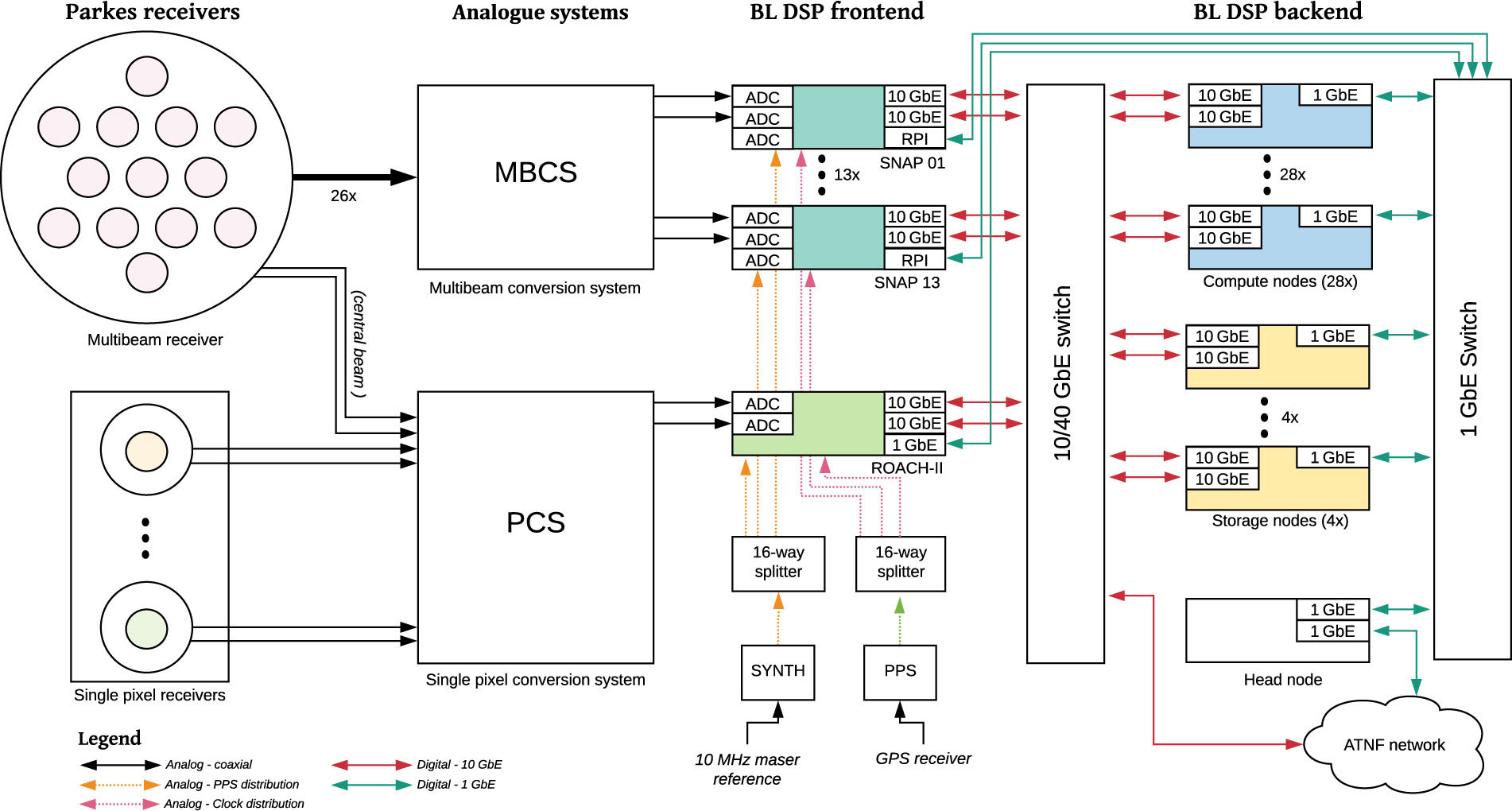
Figure 1. Block diagram of the BL data recorder system architecture at Parkes. The BL DSP backend is shared between the single-beam and multibeam DSP frontend systems.
Unlike the Green Bank installation, where the VEGAS FPGA system (Prestage et al. Reference Prestage2015) was repurposed, new hardware was installed for the DSP frontend (Section 3). As Parkes has both a single beam and multibeam conversion system, two distinct FPGA frontends have been commissioned. The first utilizes a single Collaboration for Astronomy Signal Processing and Electronics Research (CASPER) Reconfigurable Open-Architecture Compute Hardware version 2 (ROACH-II) FPGA boardFootnote d (Section 3.1) with a 5 Gsample/s analogue to digital converter (ADC) (ADC5GFootnote e), while the second utilizes a set of CASPER SNAP FPGA boardsFootnote f with in-built ADCs (Section 3.2).
During observations, BLPDR records critically sampled voltage data to disk at up to 750 MB/s per compute node. All data reduction is performed immediately after observations, with reduced data products and a subset of raw voltage data archived onto storage servers. The two FPGA frontends are connected via 10 GbE to a shared compute backend. During observations, the FPGA frontend applies coarse channelisation to the input signals and distributes channels between the backend compute servers via packetised Ethernet. A data capture code (Section 5) receives the Ethernet packets, arranges the packets into ascending time order, and writes their data payloads into an in-memory ring buffer. The ring buffer contents are then written to disk, along with telescope metadata.
2.1. Deployment timeline
The BLPDR system was deployed in several phases. In September 2016, a system comprised of two compute nodes and the PROACH-II was deployed. This allowed recording of up to 375-MHz bandwidth and was used for initial commissioning tests. A further four compute nodes and one storage server were installed on December 2016, which expanded recording capability to 1.125-GHz bandwidth; this bandwidth allowed recording of the full instantaneous bandwidth provided by the single-beam conversion system. In June 2017, the SNAP boards were installed, and the system was expanded to its full complement of 27 compute nodes plus 4 storage nodes. Observations with the multibeam system commenced in October 2017.
2.2. HIPSR commensal mode
During BLPDR commissioning, the Parkes telescope control systems were updated to support commensal observations with the HIPSR (Price et al. Reference Price, Staveley-Smith, Bailes, Carretti, Jameson, Jones, van Straten and Schediwy2016) and BLPDR systems. This upgrade was motivated by the desire to perform real-time searches for fast radio bursts (FRBs) and pulsars during BL observations with the multibeam receiver. Since commissioning, HIPSR’s capabilities have been extended to support new features such as capturing polarisation information and improving real-time FRB detection capabilities (Petroff et al. Reference Prestage2015; Keane et al. Reference Keane2018). Indeed, HIPSR is itself an upgrade of the Berkeley Parkes Swinburne Recorder (BPSR, McMahon Reference McMahon2008; Keith et al. Reference Keith2010). Nevertheless, HIPSR does not record voltage-level data products due to hardware limitations. Commensal observations therefore allow for voltage-level data products to be captured around an FRB, enabling new science.
The HIPSR real-time FRB detection system emails candidate events to a list of collaborators for verification. In the case of a bona fide FRB, the BL observer in charge is contacted to ensure that voltage data around the event is retained, and relevant follow-up observation calibration routines can be conducted as appropriate. This strategy has already been successfully used to capture the voltage data from FRB 180301 (Price et al. Reference Price2018); see Section 6.2.1.
3. Digital Hardware
The BLPDR consists of off-the-shelf Supermicro servers, Ethernet networking hardware, and FPGA processing boards developed by the CASPER (Hickish et al. Reference Hickish2016). This hardware is detailed in the following subsections.
3.1. ROACH-II FPGA board
The CASPER ROACH-II is a DSP platform centred around a Xilinx Virtex-6 series FPGA (SX475T). The ROACH-II was custom designed for radio astronomy applications and is deployed in a variety of use cases; see Hickish et al. (Reference Hickish2016) for an overview. In BLPDR, each ROACH-II is equipped with two ADC5G daughter cards and a 10 GbE SFP+ Ethernet module. This configuration is the same as the VEGAS system installed at Green Bank, as used by BLPDR’s sister instrument. As the bandwidth provided by the Parkes downconversion system is 1 GHz, a single ROACH-II board is sufficient to digitise the entire available bandwidth.
The ROACH-II board is equipped with a PowerPC microprocessor, with which monitor and control of the board is conducted. The PowerPC runs a lightweight variant of the Debian Linux operating system, provided as part of the ROACH-II board support package. The PowerPC allows for the FPGA to be reprogrammed remotely; after programming, control registers on the FPGA are presented to the PowerPC via a memory-mapped interface. The ROACH-II is controlled over the network via the use of the KATCPFootnote g protocol.
For signal digitisation, the BLPDR ROACH-II is equipped with dual CASPER ADC5G daughter cards, as described in Patel et al. (Reference Patel, Wilson, Primiani, Weintroub, Test and Young2014). The ADC5G is an 8-bit, 5 Gsample/s ADC module for the ROACH-II, and is based upon the e2V EV8AQ160 chip.Footnote h The ADC5G runs at up to 5 Gsample/s, providing up to 2.5GHz of digitised bandwidth. In BLPDR, the ADCs are configured to digitise a 1.5-GHz band. The ADC5G part was selected as it has suitable dynamic range, covers the full bandwidth of the Parkes downconversion system, and furthermore is thoroughly characterised and used widespreadly within radio astronomy.
3.2. SNAP board
The Smart Network ADC Processor, or SNAP (Hickish et al. Reference Hickish2016), is an FPGA platform primarily designed for the Hydrogen Epoch of Reionization array (HERA, DeBoer et al. Reference DeBoer2017). The SNAP board is centred around a Xilinx Kintex-7 FPGA and three on-board Hitite HMCAD1511 ADC chips.Footnote i The HMCAD1511 is a multi-input, 8-bit ADC chip that digitises four streams at up to 250 Msamples/s. Alternatively, the ADC cores may be interleaved to digitise two inputs at 500 Msample/s, or one input at 1 000 Msample/s. In the BLPDR, the 1 000 Msample/s mode is used exclusively.
In BLPDR, the 14 constituent SNAP boards are mounted vertically in a 8U VME-style chassis (Figure 2). Also housed within this chassis is a 12-power supply (Meanwell SP-480-12), which is shared between the boards. Monitor and control of each SNAP board is handled by a Raspberry Pi 2 Model BFootnote j (RPi) processor board connected via a 40-pin General purpose Input/Output (GPIO) header (Figure 3). The GPIO header provides the RPi board with 5-V power. Each RPi runs a KATCP server, via which the FPGA may be programmed and software registers may be configured.
In the BLPDR installation, each SNAP board accepts a reference clock, pulse-per-second, and two signal inputs (Figure 2). Each board digitises a dual-polarisation pair of signals from the 13 beams within the multibeam receiver; the third ADC is unused. The 14th SNAP within the Versa Module Europa (VME) chassis is configured as a spare in case of board failure.
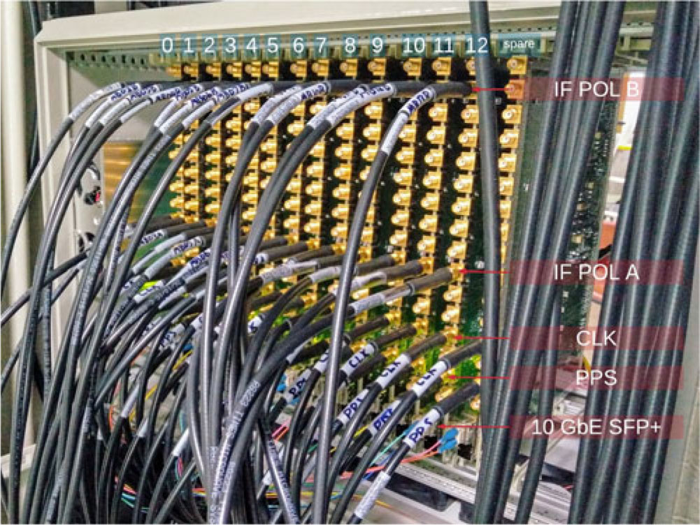
Figure 2. Front view of SNAP boards as installed at Parkes in VME-style chassis, showing analogue connections. A total of 14 boards (one per beam plus spare) are housed within the chassis.
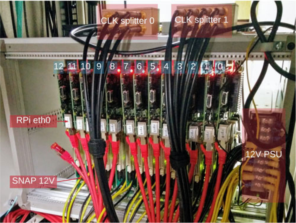
Figure 3. Rear view of SNAP boards as installed at Parkes. A Raspberry Pi 2 (RPi) is connected to each SNAP board via the GPIO pins; each RPi has a 1-GbE connection for remote monitor and control of its corresponding SNAP board.
3.3. Clock synthesiser and pulse-per-second
Each ADC requires an external reference frequency standard ‘clock signal’ to be provided. Additionally, the FPGA clock is derived from the ADC clock signal on both the SNAP and ROACH-II platforms. Clock signals for the ROACH-II ADC5G and SNAP HMCAD1511 ADC are generated by a two-channel Valon 5008 frequency synthesiser, at 3 000 and 896 MHz, respectively. For enhanced stability, the synthesiser is locked to a 10-MHz reference tone provided by an on-site maser source. To avoid frequency drift between SNAP boards, a single clock signal is distributed via a power divider network.
A nanosecond pulse-per-second (PPS) signal derived from the Global Positioning System (GPS) is also distributed to each board. The PPS allows for boards to trigger data capture on the rising edge of the PPS, synchronizing the boards to within one clock cycle (∼5 ns).
3.4. Compute servers
The BLPDR compute servers have two purposes: during observations, to capture voltage data from the FPGA frontend to disk, and between observations, to reduce voltage data into time-averaged dynamic spectra for future data analysis and for archiving. Voltage-level data products for signals of interest may also be stored.
For our purposes, this approach is advantageous over real-time data reduction as it allows use of data reduction algorithms that run slower than real time and act on file objects. Nonetheless, a real-time data analysis pipeline to run in parallel with raw data capture is under active development.
For intercompatibility with our Green Bank systems, we selected 4U Supermicro systems (Table 2), built to specification by the Australian distributor Xenon Systems. A total of 27 compute nodes (26 + 1 spare) are installed in the BLPDR system (Figure 4). The overall bandwidth that can be recorded to disk is proportional to the number of compute servers; each server may capture up to 187.5 MHz of bandwidth to disk at 8 bits per sample for two inputs (750 MB/s disk write). For the full 26-node system, an aggregate 4.875 GHz of dual-polarisation bandwidth may be captured. Each node is equipped with 24 × 5 TB hard drives, configured into two RAID 5 partitions (single parity) with two hot spares.
Table 2. BLPDR compute node configuration.
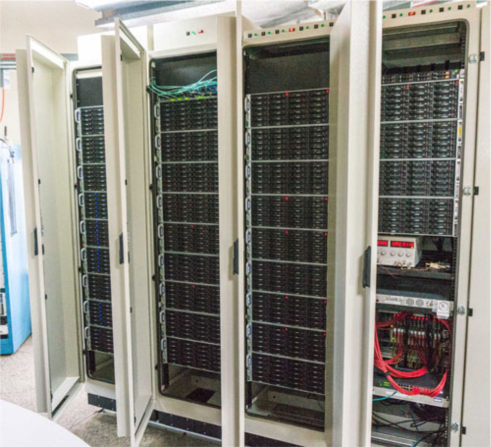
Figure 4. Rack front pic.
3.5. Storage servers
The four storage servers are similar in configuration to the compute servers (Table 3), but with a chassis that houses 36 disks, and 40-Gb Ethernet adaptors. A discrete GPU is not included.
A full complement of 36 × 6 TB hard drives are installed per server (216 TB total). Each storage server is configured with three RAID 5 arrays of 11 disks formatted with XFS; the remaining three disks are configured as global hot spares. This configuration provides 165 TB of storage per node.
Table 3. BLPDR storage node configuration.
3.6. Ethernet interconnect
The SNAP boards, ROACH-II, compute, and storage nodes are connected together via a 10-Gb Ethernet network. Nodes are connected via a Arista 7050QX-32 switch that has thirty-two 40-GbE QSFP+ ports; QSFP+ ports are broken out into four 10-GbE SFP+ ports using Fiberstore 850-nm fibre-optic breakout cables (FS48510) with a QSFP+ transceiver on one end (FS17538) and four SFP+ transceivers (FS33015) on the other ends.
The BLPDR head node is connected to the observatory-managed network via a 1-GbE connection; a secondary 1-Gb Ethernet interface on the head node connects the head node to the BLPDR private internal network, the interconnect for which is provided by a Netgear S3300 1 Gb Ethernet switch. Shielded category 6A cables are used throughout the BLPDR network, so as to conform to observatory requirements aimed at minimizing self-generated radio interference.
3.7. Power and cooling
The BLPDR system is installed on the second floor of the telescope tower, directly underneath the steerable dish structure. The BLPDR hardware is installed within four RF-tight cabinets with standard air-cooled 19-inch racks. Each rack may draw a maximum of 10 kW of 240-V AC power. The total power budget of the BLPDR is 19.6 kW; a breakdown of the power budget is given in Table 4.
Table 4. BLPDR power budget, not including cooling.
Power usage is at maximum during data reduction on the GPU cards; the cards are rated to draw up to 180 W when in operation. In practice, the GPUs draw ∼40 W when not in use and <120 W when running our reduction codes.
Cooled air is delivered at the bottom of the racks and is pulled through to the top by fans. Signals enter the rack via either BNC-type coaxial feedthroughs or radio-tight fibre-optic feedthroughs.
4. FPGA Firmware
4.1. Single-beam firmware (ROACH-II)
For single-beam observations, the BLPDR uses the same 512-channel VEGAS Pulsar Mode firmware as used in the Green Bank system; we refer the reader to MacMahon et al. (Reference MacMahon2018) for details. Briefly, the firmware digitises two inputs at 3.0 Gsample/s, then applies a 512-channel polyphase filterbank to produce ‘coarse’ channels. Subsets of 64 channels (187.5 MHz) are then sent over 10-Gb Ethernet to the compute nodes for further processing. In normal operation, the boards are configured to output six of the eight 187.5-MHz sub-bands (1.125 GHz total), to better match the ∼1 GHz of usable bandwidth from the telescope’s downconversion system.
4.2. Multibeam firmware (SNAP)
For observations with the multibeam receiver, a set of 13 SNAP boards are used to digitise, channelise, and output selected channels over 10-Gb Ethernet. The SNAP boards run a shared firmware, designed and compiled with the JASPER toolflow (Hickish et al. Reference Hickish2016), using Xilinx Vivado 2016.4 and Mathworks MATLAB/Simulink 2016b.
Each board accepts a polarisation pair from the 26 Intermediate frequency-mixed signals (IFs) provided by the multibeam downconversion system. Programmable registers on the firmware allow for each board to be uniquely identified and configured; each SNAP outputs data over 10 GbE to a different pair of compute nodes. The board firmware:
Nyquist samples the input signals at 8 bits with a sample rate of 896 MHz.
Coarsely channelises the data using a 256-point, 16-tap polyphase filterbank (PFB) running on the FPGA. The resultant 128 channels have a full-width half maximum (FWHM) of 3.5 MHz, with a complex-valued fixed-point bitwidth of 18 bits.
Requantises the PFB output down to 8 bits. A runtime-configurable equalization gain is used to allow tuning for optimal quantisation efficiency.
Buffers up selected channels (runtime configurable).
Converts selected channels into User datagram protocol (UDP) Ethernet packets and outputs them over 10 GbE.
The packetised output data are sent via the SNAP board’s 10-GbE SFP+ connector to the compute nodes for further processing.
In normal operation, the boards are configured to output 88 channels (channels 20–107), 308-MHz resultant bandwidth. Each compute node receives 44 contiguous channels (154 MHz) for a single SNAP board.
4.2.1. Diagnostic shared memory
To ensure the power levels are appropriate, sampled data may be captured at several points in the firmware design: directly after digitisation, at the output of the PFB, and after requantisation to 8 bits. This capture is done via the use of block RAMs on the FPGA that are accessible to the Raspberry Pi via memory mapping.
4.2.2. Packet format and data rate
The data payload of each UDP packet consists of four contiguous channels, with 512 frames (i.e. time samples) per packet. From slowest to fastest varying, data are arranged as frame, channel, polarisation, real/imaginary sample. The data payload is preceded by a 64-bit header, consisting of a 48-bit packet identifier, 8-bit channel identifier, and 8-bit beam identifier (ranging from 0 to 12). The packet identifier increases monotonically with time, to allow reconstruction of the voltage stream during depacketisation.
The total packet size is 8200 B; as such, jumbo frames support is required on all 10-GbE interfaces (the maximum transmission unit, MTU, must be increased to 8200 B or greater). A minimum of four channels must be selected for output, corresponding to an output data rate of 448.4 Mb/s per board. When configured for regular operations, 88 channels are output (308-Hz bandwidth), and the corresponding data rate is 9.866 Gb/s per board (128.253 Gb/s aggregate).
5. Software
5.1. Telescope integration
The Parkes telescope is controlled by the observer through a system called tcs (Telescope Control System). tcs provides a user interface through which observing schedules may be run and telescope configurations applied. The BLPDR system receives telescope metadata (pointing information, observing frequency setup, observer name, etc) from tcs via an Ethernet TCPFootnote k socket. Metadata are communicated over this socket with simple plaintext keyword–value pairs, to which a plaintext response of ‘OK’ is waited before sending the next keyword. To enable commensal observations, the tcs system was upgraded to broadcast metadata to both HIPSR and BLPDR in parallel.
A server daemon running on the BLPDR headnode responds to the messages from tcs and stores these metadata to a redisFootnote l database (Figure 5). Where required, server-specific metadata are computed from information provided by tcs, such as channel frequency values. This daemon also triggers the start and stop of data capture when relevant commands are received from tcs.
5.2. HASHPIPE data capture
The hashpipeFootnote m software package is used to capture UDP packets from the DSP frontend and write these data to disk. hashpipe is written in C and implements an in-memory ring buffer into which data are shared between processes, as detailed in MacMahon et al. (Reference MacMahon2018).
In both single-beam and multibeam mode, a copy of the hashpipe pipeline is launched on each compute server. Packetised data from the FPGA boards are sent via 10 GbE to the compute nodes (Figure 5); metadata are collected from the redis database running on the headnode. The hashpipe pipeline writes these metadata and data to files in the GUPPI raw format (Ford & Ray Reference Ford and Ray2010).
Different invocations of the hashpipe pipeline are required for the two modes of operation. For the single-beam mode, only six of the compute nodes are required to capture 1.125 GHz of digitised bandwidth from the FPGA frontend; each node captures a subset of 64 channels (187.5 MHz each). For multibeam mode, 26 compute nodes are used, each capturing a subset of forty-four 3.5 MHz channels (154 MHz per node), over 1.228–1.536 GHz.
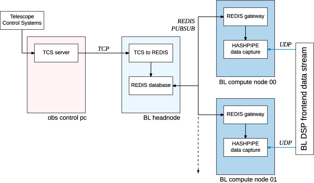
Figure 5. Block diagram showing metadata propagation from Parkes telescope control systems to BLPDR data capture processes.
5.3. GPU data reduction
In order to produce power spectral density data products, we have implemented a GPU-accelerated data reduction pipeline called bunyipFootnote n using the bifrost framework (Cranmer et al. Reference Cranmer2017). This code, in order of operation:
Reads data from file in GUPPI raw format.
Performs a fast Fourier Transform (FFT). This operation is performed on the GPU device, using the NVIDIA cufft library.
Squares the output, and integrates the data in GPU device memory.
Combines polarisations to form Stokes-I data.
Writes output data to file in either Sigproc filterbankFootnote o format or HDF5Footnote p format.
For multibeam observations, the pipeline produces three products with different time and frequency resolution pairs: (3.37 Hz, 19.17 s); (3.42 kHz, 0.60 s); (437.5 kHz, 292.57 μs). For single-beam observations, resolutions are: (2.79 Hz, 18.25 s); (2.86 kHz, 1.07 s); (366 kHz, 349.53 μs). Data formats will be detailed further in Lebfosky et al. (in preparation).
6. Verification and Results
6.1. Single-beam observations
The single-beam system uses the same digitiser and FPGA firmware as the Green Bank install; as such, we followed the same verification procedures detailed in MacMahon et al. (Reference MacMahon2018). We first verified data throughput through Ethernet UDP capture tests and benchmarking disk write speed. We then confirmed the probability distribution for digitised on-sky data was Gaussian, as expected for noise-dominated astrophysical signals. By injection of test tones, we confirmed our frequency metadata was correct to better than the width of our highest-resolution data product (2.79 Hz).
Here, we present a sampling of results that are illustrative of system performance.
6.1.1. Proxima Centauri
At a distance of 4.2 light years, Proxima Centauri is the nearest star to Earth, after the Sun. In August 2016, the discovery of an Earth-sized exoplanet orbiting Proxima Centauri within the so-called ‘habitable zone’ was announced by Anglada-Escudé et al. (Reference Anglada-Escudé2016). This makes Proxima Centauri an interesting candidate for SETI observations.
We observed Proxima Centauri for 5 min on 2017 January 20, using the 10-cm receiver. Five compute nodes were used to record 187.5 MHz of voltage data each, spanning between 2.6–3.5375 GHz (937.5 MHz total). Stokes-I spectra (2.86 kHz, 1.07 s) from the observation were created using our GPU-accelerated pipeline.
The 5-min time-averaged spectrum from Proxima Centauri is shown in Figure 6. The inset shows the characteristic filter shape of the coarse channels; the filter shape of the telescope’s downconversion system can be seen at the band edges. These data are typical of 10-cm observations. Our observations and data analysis of Proxima Centauri and other nearby star targets as listed in Isaacson et al. (Reference Isaacson2017) are ongoing and will be the subject of a future publication.
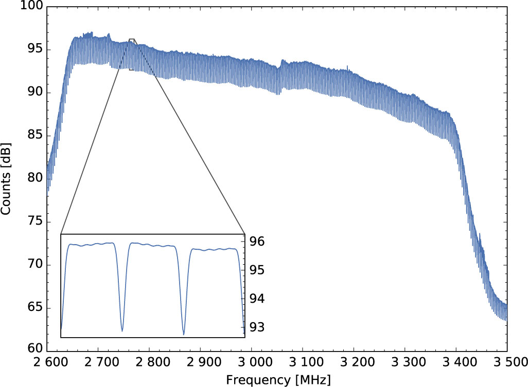
Figure 6. Uncalibrated mid-resolution (327 680 channels over 937.5 MHz) spectrum on Proxima Centauri, using the 10-cm receiver on 2017 January 20. The inset shows a zoom over three coarse channels, showing the characteristic filter shape.
6.1.2. J0835-4510 (Vela) single pulses
PSR J0835-4510—the Vela Pulsar—is the brightest pulsar in the Southern sky. PSR J0835-4510 has a period of 89.33 ms, mean flux density of 1 100 mJy at 1.4 GHz, and dispersion measure (DM) of 67.97 pc cm−3 (Manchester et al. Reference Manchester, Hobbs, Teoh and Hobbs2005).
We observed PSR J0835-4510 for 5 min using the 10-cm receiver and BLPDR system, on UTC 2017 July 7 at 07:04. The data were recorded across five compute nodes, reduced into Stokes-I filterbank files with 366 kHz, 349.53-μs resolution, then combined to form a single filterbank file spanning 2.6–3.4 GHz. Two broadband pulses from these observations are shown in Figure 7. The resultant period, DM, and other parameters for PSR J0835-4510 are consistent with previously known values.
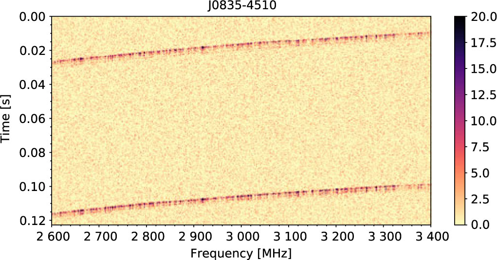
Figure 7. Two broadband pulses at 10-cm wavelength from the Vela pulsar (PSR J0835-4510, MJD 57941.295), after bandpass removal. Colour scale is flux in Jy, calibrated using an (approximate) 38.5 Jy system equivalent flux density for the 10-cm receiver.
6.1.3. Voyager 2
Voyager 2 is a NASA space probe launched on 1977 August 20. Currently, at a distance of over 116 AU from Earth, Voyager is one of the most distant human-made objects, but its narrowband telemetry signal can still be detected. This makes observations of Voyager 2 an excellent test of the BLPDR capabilities.
We observed Voyager 2 on UTC 2016 October 10 at 09:37, using the Parkes Mars receiver (8.1–8.5 GHz). The J2000 ephemeris at observation, retrieved from the NASA HORIZONS websiteFootnote q, was (19:58:36, −57:18:53.5). Using BLPDR, we recorded 5 min of data and created Stokes-I filterbank files with 2.79-Hz resolution. Figure 8 shows the detected telemetry signal; the carrier, upper, and lower sidebands are clearly visible. Here, we have not corrected for doppler broadening of the signal.
Figure 8. Voyager 2 space mission telemetry signal at UTC 09:37 2016 October 10, detected using the Parkes Mars receiver and the BLPDR.
6.2. Multibeam observations
The BLPDR system receives a total of 26 inputs from the multibeam conversion system. A set of configurable attenuators in the conversion system allows for power levels at the ADCs to be matched; we aim for input powers of −20 dBm and run the ADCs with a 8× digital gain such that input RMS levels are between 8 and 16 counts. This level provides high quantisation efficiency (better than 99%), while leaving >5 bits of headroom for radio interference.
Figure 9 shows example spectra for all 13 beams, taken from a 5-min observation of globular cluster NGC 1851 (RA 5:14:06, DEC −40:02:47), on UTC 2018 February 27 at 05:35; globular clusters were identified as potential ‘cradles of life’ by Di Stefano & Ray (Reference Di Stefano and Ray2016). As in Figure 6, the coarse bandpass filter shape can be seen. Sources of radio interference (RFI) can be identified as common to all beams.
Figure 9. Example Stokes-I spectra from BLPDR showing bandpass for the 13 beams of the 21-cm multibeam receiver; plots are laid out in the same hexagonal manner as the receiver. Here, beam 1 is centred on globular cluster NGC 1851 (J2000 coordinates RA 5:14:06, DEC − 40:02:47).
6.2.1. FRB 180301
On 2018 March 01 at UTC 07:34, an FRB was detected by the commensal HIPSR real-time system during BL observations with the multibeam receiver (Price et al. Reference Price2018). An email trigger was broadcast by the HIPSR system to the SUPERB collaboration (Keane et al. Reference Keane2018) and BL for verification, and the observer in charge was notified within minutes so that calibration routines could be performed. The burst, FRB 180301 (Figure 10), was detected ∼6° below the Galactic plane, at J2000 RA 06:12:40, with an uncertainty of ±20 s, and declination +04:33:40, within an uncertainty of ±20 arcsec. The burst was detected in beam 3 of the receiver, with an observed signal-to-noise ratio of 16, a ∼0.5-Jy peak flux density, ∼3-ms burst width and DM of ∼521 pc cm−3.
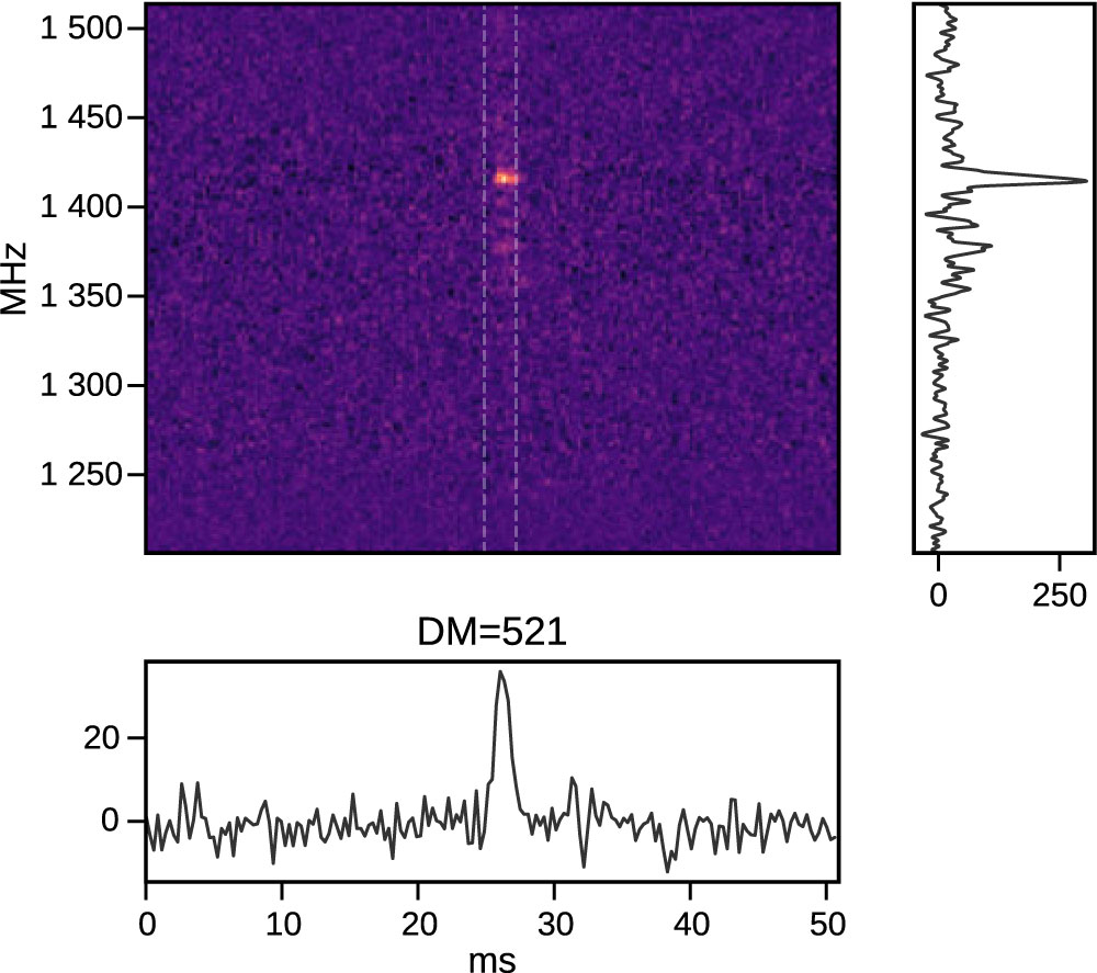
Figure 10. Incoherently dedispersed spectrum of FRB 180301. Dedispersed time series using a DM of 521 pc cm−3 plotted at the bottom. The average frequency structure of the pulse, within the dashed lines of the dynamic spectrum, is plotted on the right. Frequency structure and time series are in arbitrary flux units.
The BLPDR recorded the voltage data for this burst from each of the 13 beams of the receiver, all of which have been saved for analysis. These voltage-level products allow for coherent dedispersion of the FRB, measurement of its rotation measure, polarisation properties, and localisation via inter-beam correlation. Analyses of FRB 180301 are ongoing and will be the subject of a future publication (Price et al., in preparation).
7. Discussion
7.1. SETI survey speed
In Enriquez et al. (Reference Enriquez2017), various figures of merit are discussed for SETI surveys; for comparison of an instrument’s intrinsic capability, the survey speed figure of merit (SSFM) is the most salient. The SSFM quantifies how fast a telescope can reach a target sensitivity, S min, for a given (narrowband) observation:
 \begin{equation}{\text{SSFM}} \propto \frac{{\Delta {\nu _{{\text{obs}}}}}}{{{\text{SEF}}{{\text{D}}^2}\delta \nu }},\end{equation}
where Δν obs is the instantaneous bandwidth of the instrument, δν is the channel bandwidth, and SEFD is the system equivalent flux density.
The parameters δν and Δν obs are set by the capabilities of the digital systems (although constrained by the receiver), whereas the SEFD is determined by the telescope’s collecting area and system temperature. As BLPDR records voltages, the minimum channel resolution is constrained only by the observation length (δν ∝ t −1). Table 5 gives a comparison of BLPDR to other digital systems at Parkes; in comparison to the Project Phoenix (Tarter Reference Tarter1996) and SERENDIP South (Stootman et al. Reference Stootman, De Horta, Oliver and Wellington2000) digital systems, the ratio Δν obs / δν is over 104 larger. For this comparison, the channel resolution at maximum instantaneous bandwidth is used. Note that for an FFT-based spectrometer, the ratio Δν obs / δν is equal to the total number of channels.
Table 5. Comparison of channel bandwidth and instantaneous bandwidth—that is, aggregate Δν obs over all beams—for digital backends at Parkes.
a Minimum resolution for 30-min observation.
7.2. Conclusions
BLPDR is a new digital system for the CSIRO Parkes 64-m telescope that can record up to an aggregate of 8.624 GHz of 8-bit data at data rates of up to 128 Gb/s. This places it as the second highest maximum data recording rate of any radio astronomy instrument, after its sister installation in Green Bank (see Table 5 of MacMahon et al. Reference MacMahon2018).
The BLPDR system is being used to undertake targeted observations of nearby stars and galaxies, and a Galactic plane survey; details of the survey strategy may be found in Isaacson et al. (Reference Isaacson2017). These observations, and related data analyses, are ongoing.
Through commensal observations with the HIPSR real-time FRB system, voltage data for transient events may be captured and analysed. This strategy allowed the capture of voltage data from FRB 180301, which will be the subject of a future publication. The ability to capture voltage data opens opportunities for other ancillary science, which may be supported on a shared-risk basis.
In the coming months, a 0.7–4 GHz receiver will be installed at the Parkes telescope. This receiver will be digitised in the focus cabin, and data will be sent via 10 GbE to a GPU-based spectrometer that is under development by the Australian Telescope National Facility (ATNF). A copy of these data will also be multicast to BLPDR for SETI science; only modest modifications to the BLPDR data capture codes will be required to support this new functionality.
Author ORCIDs.
Danny C. Price, http://orcid.org/0000-0003-2783-1608.
Acknowledgements
Breakthrough Listen is managed by the Breakthrough Initiatives, sponsored by the Breakthrough Prize Foundation. The Parkes radio telescope is part of the Australia Telescope National Facility which is funded by the Australian Government for operation as a National Facility managed by CSIRO. V. G. would like to acknowledge NSF grant no. 1407804 and the Marilyn and Watson Alberts SETI Chair funds. This work makes use of hardware developed by the Collaboration for Astronomy Signal Processing an Electronics Research (CASPER). D. Price thanks Matthew Bailes and Willem van Straten for site visits and discussions.


