


Introduction
Weeds are ever-present pests of cotton production in Australia, with glyphosate-tolerant and glyphosate-resistant weeds becoming increasingly problematic over time because of overreliance on glyphosate in the farming system, combined with a reduction in the use of other weed control tactics (Charles et al. Reference Charles, Sindel, Cowie and Knox2020a; Koetz Reference Koetz, Maas and Redfern2019a; Werth et al. Reference Werth, Boucher, Thornby, Walker and Charles2013). The increase in weed issues over the past decade has necessitated the return to a more integrated weed management (IWM) system on many cotton farms, with the increasing use of residual herbicides, interrow cultivation, and hand hoeing (Koetz Reference Koetz, Maas and Redfern2019b). One of the concepts that could facilitate the adoption of an IWM system would be a weed control threshold, enabling cotton growers to optimize the timing of their weed control inputs (Knezevic and Datta Reference Knezevic and Datta2015; Knezevic et al. Reference Knezevic, Evans, Blankenship, Van Acker and Lindquist2002; Korres and Norsworthy Reference Korres and Norsworthy2015). A weed control threshold would help cotton growers balance the need to control weeds before they become problematic, against practical considerations such as the availability of equipment and labor and the costs of weed control, including the potential costs of crop damage and off-target herbicide movement. Weeds need to be controlled before they set seed and before weed competition increases to the level at which it results in yield reductions. However, weed control inputs need to be managed to minimize the number of inputs needed over the crop-growing season, and to reduce costs and negative production, and environmental effects (Taylor et al. Reference Taylor, Charles, Inchbold and Swanepoel2004). A weed control threshold will help cotton growers balance those needs.
Pest control thresholds have been widely used in cotton production in Australia, starting with the introduction of SIRATAC, a pest threshold-based tool introduced in the 1980s for managing heavy infestations of insecticide-resistant helicoverpa (Helicoverpa armigera and H. punctigera; Hearn and Bange Reference Hearn and Bange2002). Since then, pest control thresholds have been adopted for all major insect and mite pests of cotton in Australia, with individual thresholds developed for each species or group of closely related species (Grundy Reference Grundy, Maas and Redfern2019). The need for individual thresholds has been necessitated by the widely varying impacts of different insects. Thrips (Thrips tabaci, Frankliniella schultzei, F. occidentalis), for example, can cause unacceptable early-season damage to cotton, but at low numbers they can be beneficial to the crop later in the season because they are key predators of spider-mite (Tetranychus urticae) eggs, another major pest species (Grundy Reference Grundy, Maas and Redfern2019). Spider mites are generally a later-season pest, with the threshold modified according to the expected length of the growing season for the differing cotton-growing regions. Hence, different thresholds are applied to thrips and mites because these pests impact the cotton crop in very different ways.
A multispecies weed control threshold should, at least conceptually, be simpler to develop than generalized insect thresholds, because most weeds have similar competitive effects on a crop, with the level of damage caused by plant competition most closely related to the time of weed emergence (relative to crop emergence) and duration of competition, weed density, and weed size (Askew and Wilcut Reference Askew and Wilcut2001, Reference Askew and Wilcut2002a, Reference Askew and Wilcut2002b; Cortés et al. Reference Cortés, Mendiola and Castejón2010; Fast et al. Reference Fast, Murdock, Farris, Willis and Murray2009; Korres and Norsworthy Reference Korres and Norsworthy2015; Ma et al. Reference Ma, Yang, Wu, Jiang, Ma and Ma2016; Scott et al. Reference Scott, Askew, Wilcut and Brownie2000; Webster et al. Reference Webster, Grey, Flanders and Culpepper2009). The impact of weed competition on a crop can also be affected by factors such as seasonal variation (Bukun Reference Bukun2004), soil moisture (Tingle et al. Reference Tingle, Steele and Chandler2003; Vencill et al. Reference Vencill, Giraudo and Langdale1993), soil fertility (Robinson Reference Robinson1976; Tursun et al. Reference Tursun, Datta, Tuncel, Kantarci and Knezevic2015), row spacing (Tursun et al. Reference Tursun, Datta, Budak, Kantarci and Knezevic2016), and crop health (Buchanan et al. Reference Buchanan, Crowley and McLaughlin1977; Webster and Davis Reference Webster and Davis2007). However, in fully irrigated cotton production in Australia, most of these factors are maintained as closely as possible to optimum, such that these factors should normally have little influence on the crop’s response to weed competition. Hence, a generalized weed control threshold model for irrigated cotton in Australia might be possible if the model is able to account for the time of weed emergence, duration of weed growth, weed density, and weed size (Charles et al. Reference Charles, Sindel, Cowie and Knox2019a).
Defining the critical period for weed control (CPWC) is an important step in developing an IWM program for a crop and a way to delineate a dynamic weed control threshold model (varying over the crop-growing season) that incorporates the effects of the time of weed emergence (relative to crop emergence) and the duration of weed growth on crop yield (Knezevic and Datta Reference Knezevic and Datta2015). Previous competition studies have shown that other factors can also affect crop yield, such as weed density, weed height, and weed biomass (Askew and Wilcut Reference Askew and Wilcut2001, Reference Askew and Wilcut2002a, Reference Askew and Wilcut2002b; Cortés et al. Reference Cortés, Mendiola and Castejón2010; Fast et al. Reference Fast, Murdock, Farris, Willis and Murray2009; Scott et al. Reference Scott, Askew, Wilcut and Brownie2000), but these terms have not been included in CPWC models.
Historically, CPWC models have been site, season, species, and density specific (Charles et al. Reference Charles, Sindel, Cowie and Knox2019b). Knezevic and Datta (Reference Knezevic and Datta2015) suggest using growing degree days (GDD) as the measure of time to reduce seasonal differences, and Charles et al. (Reference Charles, Sindel, Cowie and Knox2019b, Reference Charles, Sindel, Cowie and Knox2020a, Reference Charles, Sindel, Cowie and Knox2020b) reported that using GDD as the time descriptor overcame the effects of season on the CPWC relationship in fully irrigated cotton in Australian conditions. In an additional step, Charles et al. (Reference Charles, Sindel, Cowie and Knox2019b, Reference Charles, Sindel, Cowie and Knox2020a, Reference Charles, Sindel, Cowie and Knox2020b) included weed density as an extra term in the equations used to define the CPWC, and so were able to account for this factor in their CPWC models. In addition, Charles et al. (Reference Charles, Sindel, Cowie and Knox2020a) tested the possibility of using weed height or weed biomass (kilograms of aboveground dry matter per square meter) in place of weed density in their CPWC models and found that the critical time for weed removal (CTWR) relationship was improved for the mimic weed mungbean in fully irrigated cotton when weed biomass was used in the model. The substitution of weed biomass for weed density gave no improvement in the critical weed-free period (CWFP) relationship.
Thus, Charles et al. (Reference Charles, Sindel, Cowie and Knox2020a) were able to fulfil the theoretical requirement for a more generalized weed control threshold for irrigated cotton, incorporating the time of weed emergence, duration of competition, weed density and size into their extended CPWC model, because weed biomass (kg m−2) includes components of weed size and weed density. The objective for this study was to determine whether this approach of including weed density and size in the CPWC model could be applied to other weeds with different morphologic characteristics, and in addition, whether this approach would allow a more generalized model to be developed that could be applied across a range of weed species and types.
Materials and Methods
Field studies were conducted at the Australian Cotton Research Institute, Narrabri (30.12°S, 149.36°E; elevation 201 m) on a heavy alluvial clay (fine, thermic, smectitic, Typic Haplustert) soil. Cotton crops were grown over six seasons from 2003 to 2016, in line with standard commercial practices using commercial cotton cultivars on raised hills, 1 m apart. Fields were fertilized with 180 kg N ha−1, applied before planting, and were flood-irrigated as required.
Experimental Design
Within each season, the experiments used a randomized, complete block design with split plots and four replications; subplots were 4 rows (4 m) wide by 10 m in length. Main plots were times of weed planting and removal, and subplots were weed densities. The mimic weeds common sunflower, Japanese millet, and mungbean were individually planted with the crop or at predetermined periods after crop emergence, sown to achieve target densities. The times of weed planting and removal were measured in GDD since planting, defined as:
 $$T = \mathop \sum \nolimits {{\left( {{t_{min}}{\rm{}} + {\rm{}}{t_{max}}} \right)} \over 2} - {t_b}$$
where t min and t max were the daily minimum and maximum air temperatures, respectively, and t b was the base temperature of 15.5 C (Bukun Reference Bukun2004).
Weed planting and removal times were planned to occur at 150, 300, 450, 600, 750, and 900 GDD. Actual densities of established weeds, and times of planting and removal, were influenced by rainfall and irrigation events, with weed emergence delayed by inadequate soil moisture on some occasions. Not all target weed densities were achieved in all seasons.
Weed density and height were recorded at the time of weed removal and plants were weighed after drying at 70 C for at least 72 h in a forced-air oven. Cotton was mechanically harvested, and a single-saw gin was used to determine ginning percentage and lint yield. Additional details of the experiments are described in Charles et al. (Reference Charles, Sindel, Cowie and Knox2019b, Reference Charles, Sindel, Cowie and Knox2020a, Reference Charles, Sindel, Cowie and Knox2020b).
Statistical Analysis
The data sets used by Charles et al. (Reference Charles, Sindel, Cowie and Knox2019b, Reference Charles, Sindel, Cowie and Knox2020a, Reference Charles, Sindel, Cowie and Knox2020b) were analyzed using R statistical software, version 3.6.3 (R Foundation for Statistical Computing, Vienna, Austria) with a significance level of P < 0.05. Regression analysis was used to test the relationships between the relative cotton-lint yield (i.e., lint yield relative to the weed-free control in each season); and weed density, biomass, and height, using the coefficient of determination (r 2) to assess the fit of each model. Data were fit to Gompertz, logistic and exponential functions as described by Charles et al. (Reference Charles, Sindel, Cowie and Knox2019b, Reference Charles, Sindel, Cowie and Knox2020b), with the exponential function substituted for the logistic function where the shape of the curve did not allow the logistic function to be fit, or where the exponential function improved the fit of the data, as indicated by the Akaike information criterion (AIC). Weed density, height, and biomass were then fit to the CPWC relationships described by Charles et al. (Reference Charles, Sindel, Cowie and Knox2019b, Reference Charles, Sindel, Cowie and Knox2020b) using the AIC to determine the model with the best fit. The CTWR models were constrained to 100% relative yield where no weeds were present.
Data sets from all three mimic weeds, common sunflower (Charles et al. Reference Charles, Sindel, Cowie and Knox2019b), Japanese millet (Charles et al. Reference Charles, Sindel, Cowie and Knox2020b), and mungbean (Charles et al. Reference Charles, Sindel, Cowie and Knox2020a) were combined in the present study to test whether a multispecies CPWC model could be fit to the combined data set. Linear regression was used to test the association between relative cotton-lint yield and experimental year; weed species, density, biomass, and height; time of emergence; and time of removal. The data were combined over years because experimental year was not a significant factor in the regression. The combined data set was used to develop new multispecies CTWR and CWFP models. The fit of these multispecies models was tested over the three weed species by using the functions to generate predicted lint-yield reductions for each species and contrasting the predicted to the observed yield reductions. A simple linear model was fit to this contrast of predicted and observed yield reductions for each species and 95% confidence intervals of the lines were generated. The fitted lines for each species were compared with a line generated for the combined data set and the overlap of the confidence intervals was examined.
Results and Discussion
Developing Dynamic Models for the Mimic Weed Common Sunflower
A dynamic relationship was developed by Charles et al. (Reference Charles, Sindel, Cowie and Knox2019b) to define the CPWC for common sunflower, a large mimic weed, in high-yielding cotton, using weed density and the duration of weed competition as descriptive elements in the models. However, more recent research using mungbean, a smaller broadleaf mimic weed, found that the relationships could be improved by substituting weed biomass (kg m−2) for weed density (plants m−2; Charles et al. Reference Charles, Sindel, Cowie and Knox2020a). Charles et al. (Reference Charles, Sindel, Cowie and Knox2020a) also tested weed height and combinations of weed density, height, and biomass as factors, but found the best fit with weed biomass. Weed biomass and weed height had previously been shown to be correlated to cotton-lint yield (Askew and Wilcut Reference Askew and Wilcut2001, Reference Askew and Wilcut2002a, Reference Askew and Wilcut2002b; Charles et al. Reference Charles, Sindel, Cowie and Knox2019a; Cortés et al. Reference Cortés, Mendiola and Castejón2010; Fast et al. Reference Fast, Murdock, Farris, Willis and Murray2009).
Using the data published by Charles et al. (Reference Charles, Sindel, Cowie and Knox2019b), we tested the relationships between relative cotton-lint yield and weed (common sunflower) biomass, height, and density. There were strong associations between the relative lint yield and weed biomass (r 2 = 0.69), and height (r 2 = 0.68), with weed biomass being the stronger relationship (Figure 1), but no apparent relationship with weed density (r 2 = 0.02).

Figure 1. The influence of common sunflower (A) biomass, and (B) plant height on relative cotton-lint yield. Parameters of the models are as follows: y is the relative crop yield; B is the above-ground weed biomass; and H is the weed height. Data points for the relationships are treatment means.
We tested the fit of weed density, height, and biomass on the dynamic relationships defining the CPWC for common sunflower using the data published by Charles et al. (Reference Charles, Sindel, Cowie and Knox2019b) and found the fit of both the CTWR and CWFP relationships was most improved by substituting weed biomass for weed density (Figure 2). The CPWC defined by these curves extended from 21 GDD to 1,244 GDD for 10 g weed m−2 when a 1% weed control threshold was applied, and for the full season (2 GDD to picking) with 2.5 kg weed m−2, the maximum dry aboveground biomass of common sunflower reported by Charles et al. (Reference Charles, Sindel, Cowie and Knox2019b). Our model shows that the presence of 1.09 kg m−2 or more of weeds at any stage during the season (4 GDD to 1,600 GDD) reduced the cotton-lint yield by more than the 1% threshold.

Figure 2. The critical period for weed control (CPWC) for common sunflower competing with cotton. The CPWC is defined by the intersection of the CTWR (green lines), and CWFP (blue lines), with a 1% yield-reduction threshold (horizontal dashed line). The derived relationships for common sunflower biomass of 10, 200, 500, 1,000, and 2,500 kg m−2 are presented as examples. Parameters of the curves are as follows: y is the relative lint yield; T is the cumulative degree days since planting; and B is the aboveground weed biomass. Data points for the relationships are treatment means. The horizontal solid line indicates the weed-free yield. The limits of the derived CPWC curves for 10 and 2,500 g m−2 are shown by the vertical dashed red lines and bracketed values. Points of minimum yield loss for 10 and 2,500 g m−2 are indicated by the dashed purple lines and bracketed values. CTWR, critical time for weed removal; CWFP, critical weed-free period.
This model, based on weed biomass, is both a statistical and practical improvement over the original CPWC model based on weed density (Charles et al. Reference Charles, Sindel, Cowie and Knox2019b) because it includes a measure of weed size (biomass), allowing for variation in the size and the growth rate of the weeds, and allowing for the possibility that the model might be more widely applied to a range of weed species and types, with similar morphologic traits. This possibility of developing a multispecies competition model was proposed by Charles et al. (Reference Charles, Sindel, Cowie and Knox2019a), who developed a simple model relating cotton-lint yield loss to a combination of weed height and weed biomass for three very different mimic weed species: common sunflower; mungbean; and Japanese millet.
Developing Dynamic Models for the Mimic Grass Weed Japanese Millet
A dynamic relationship defining the critical period for weed control for Japanese millet, a mimic grass weed, in high-yielding cotton was developed by Charles et al. (Reference Charles, Sindel, Cowie and Knox2020b) using weed density and the duration of weed competition as descriptors in the models. Using these data, we tested the relationships between the relative lint yield and weed biomass, height, and density, with the data averaged over the remaining factors. The results mirrored the earlier findings with common sunflower, with lint yield associated with weed biomass (r 2 = 0.46) and weed height (r 2 = 0.4; Figure 3), but poorly related to weed density (r 2 = 0.04).
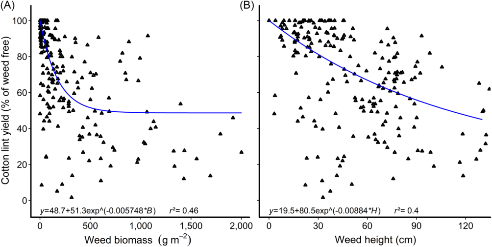
Figure 3. Reduction in cotton-lint yield with increasing Japanese millet (A) biomass and (B) height. Parameters of the models are as follows: y is the relative crop yield; B is the aboveground weed biomass; and H is the weed height. Data points for the relationships are treatment means.
We tested the fit of weed density, biomass, and height on the CPWC relationships for Japanese millet published by Charles et al. (Reference Charles, Sindel, Cowie and Knox2020b) and found an improvement in the fit of the CTWR when weed biomass was substituted for weed density, but no improvement in the CWFP relationship with any combination of weed density, biomass, or height (Figure 4). Charles et al. (Reference Charles, Sindel, Cowie and Knox2020a) similarly reported that the CTWR relationship for mungbean was improved when weed biomass was substituted for weed density in the relationship, but that the CWFP model was not improved by substituting either weed biomass or weed height into the relationship. The CPWC defined for Japanese millet using the new CTWR curve begins earlier in the season than the original CPWC (Charles et al. Reference Charles, Sindel, Cowie and Knox2020b), beginning at 26 GDD with 10 g weed m−2 and 8 GDD with 2 kg weed m−2. There was no substantial change in the points of minimum yield loss with the new model.

Figure 4. The critical period for weed control (CPWC) for Japanese millet competing with cotton. The CPWC is defined by the intersection of the critical time for weed removal (CTWR; green lines), and critical weed-free period (CWFP; blue lines), with a 1% yield-reduction threshold (horizontal dashed line). The derived relationships for Japanese millet biomass of 10, 200, 500, 1,000, and 2,000 kg m−2 are presented as examples for the CTWR relationship, and Japanese millet densities of 10, 20, 50, 100, and 200 plants m−2 are presented as examples of the CWFP relationship. Parameters of the curves are as follows: y is the relative lint yield; T is the cumulative degree days since planting; B is the aboveground weed biomass, and D is the weed density. Data points for the relationships are treatment means. The horizontal solid line indicates the weed-free yield. The limits of the derived CPWC curves for 10 and 2,000 g m−2 (CTWR), and 10 and 200 weeds m−2 (CWFP), are shown by the vertical dashed red lines and bracketed values. Points of minimum yield loss for 10 weeds and 10 g m−2, and 200 weeds and 2,000 g m−2, are indicated by the dashed purple lines and bracketed values.
Developing Dynamic Models Using the Combined Data Sets for Three Mimic Weeds
To test the possibility of developing a multispecies competition model for irrigated cotton, we combined the data sets for the mimic weeds common sunflower (Charles et al. Reference Charles, Sindel, Cowie and Knox2019b), Japanese millet (Charles et al. Reference Charles, Sindel, Cowie and Knox2020b), and mungbean (Charles et al. Reference Charles, Sindel, Cowie and Knox2020a). We tested the associations between relative cotton-lint yield and experimental year; and weed species, density, biomass, height, time of emergence, and time of removal. Experimental year was not a significant factor in the regression, but all other factors were significantly associated with lint yield. Weed density and weed species, however, were only weakly related to relative yield (r 2 = 0.003 and r 2 = 0.04, respectively).
The relative lint yield of cotton was most strongly associated with weed height (r 2 = 0.59) and weed biomass (r 2 = 0.38), with the times of weed emergence and weed removal less strongly related, r 2 = 0.09 and r 2 = 0.15, respectively. The relationship improved when the times of weed emergence and weed removal were both included in the regression (r 2 = 0.33). The correlations of lint yield with weed height and biomass, and the times of weed emergence and removal, were further improved by using exponential (weed height and biomass; Figure 5), and Gompertz functions (times of weed emergence and removal).

Figure 5. Cotton-lint yield as a function of (A) weed height and (B) weed biomass for the combined data sets from common sunflower, Japanese millet, and mungbean competition. Parameters of the models are as follows: y is the relative crop yield; B is the aboveground weed biomass; and H is the weed height. Data points for the relationships are treatment means.
Using the combined data set, we developed new CTWR and CWFP relationships with weed density, biomass, and height as factors separately and in combination. The best fit for both relationships occurred when weed height and biomass were included as factors by developing a multispecies CPWC model (Figure 6) in line with the findings of Charles et al. (Reference Charles, Sindel, Cowie and Knox2019a) who also related relative lint yield to weed height and biomass. The CPWC derived from the multispecies models extended from 49 to 1,187 GDD for weeds 1 cm tall and weighing 10 g m−2, and for the full season (3 GDD to picking) with weeds that were 2 m tall and 2 kg m−2 biomass. The presence of weeds that were 85 cm tall and of 850 g m−2 biomass or more reduced the cotton-lint yield at any stage in the season (to 1,600 GDD) by more than the 1% yield-loss threshold. The reduction in cotton-lint yield below the 1% yield-loss threshold was similarly caused by weeds of any height (1 cm or more) where weed biomass exceeded 2,010 g m-2, or any biomass (10 g m−2 or more) where weed height exceeded 145 cm.
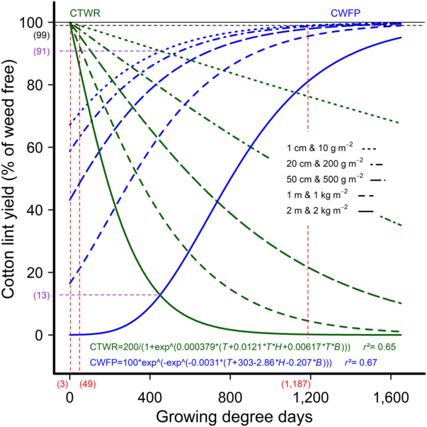
Figure 6. The critical period for weed control (CPWC) for cotton using a multispecies model. The CPWC is defined by the intersection of the critical time for weed removal (CTWR; green lines), and critical weed-free period (CWFP; blue lines), with a 1% yield-reduction threshold (horizontal dashed line). Parameters of the models are as follows: y is the relative lint yield; T is the cumulative degree days since planting; H is the weed height; and B is the aboveground weed biomass. The derived relationships for weed height and biomass of: 1 cm and 10 g m−2; 20 cm and 200 g m−2; 50 cm and 500 g m−2; 1 m and 1 kg m−2; and 2 m and 2 kg m−2 are presented as examples. The horizontal solid line indicates the weed-free yield. The limits of the derived CPWC curves for weeds 1-cm tall and 10 g m−2 biomass, and 2-m tall and 2 kg m−2 are shown by dashed red lines and bracketed values. The points of minimum yield loss for weeds 1-cm tall and 10 g m−2 biomass, and 2-m tall and 2 kg m−2 are indicated by the dashed purple lines and bracketed values.
We tested the fit of the CWFP model by comparing observed and predicted yield reductions for each species against the combined data set. The 95% confidence intervals for common sunflower and Japanese millet overlap the confidence interval for the combined data set throughout its length, indicating that the multispecies model reasonably predicts the yield loss of these two very different mimic weeds: a large broadleaf weed and a much smaller grass weed (Figure 7). The confidence interval for the combined data set overlaps the confidence interval for mungbean for relative yields of 40% or more. The multispecies model overestimates the yield loss from competition from mungbean below 40% relative yield, although the difference between the two confidence intervals was very small, and increased to 1% of relative yield at the lowest observed yield of 7%. We also note that the multispecies CWFP model underestimates all yield losses below 71% relative yield (the relationship is above the 1:1 line) and overestimates yield losses at higher yields. This inaccuracy appears to be caused by the nature of the model used. Future work should explore alternative mathematical relationships to correct this issue with our model. Nevertheless, we contend that the multispecies CWFP model reasonably represents the competition relationships of these very different mimic weeds.

Figure 7. Estimated linear relationships and 95% confidence intervals for observed and predicted relative crop yield using the multispecies critical weed-free period model for (A) common sunflower, (B) mungbean, and (C) Japanese millet. The relationship (D) for the combined data set and each species is shown against a 1:1 line. Data points for the relationships are treatment means.
We similarly tested the fit of the CTWR model by comparing observed and predicted yield reductions for each species against the combined data set. The 95% confidence interval for the combined data set overlapped the confidence intervals for all three mimic weeds throughout their length, indicating that the multispecies model reasonably predicted the yield loss of these weeds (Figure 8). Again, we note that the multispecies CTWR model underestimates yield losses below 68% relative yield (the relationship is above the 1:1 line) and overestimates yield losses at higher yields. Correcting this inaccuracy should be an aim of future work.

Figure 8. Estimated linear relationships and 95% confidence intervals for observed and predicted relative crop yield using the multispecies critical time for weed removal model for (A) common sunflower, (B) mungbean, and (C) Japanese millet. The relationship (D) for the combined data set and each species is shown against a 1:1 line. Data points for the relationships are treatment means.
Further Development of a Multispecies Model
A multispecies CPWC model will be a valuable tool for developing IWM systems in irrigated cotton, enabling Australian cotton growers to optimize their weed control inputs (Knezevic and Datta Reference Knezevic and Datta2015). The multispecies model developed in this study was generated from data from three very dissimilar mimic weed types and so should be applicable to many of the weed species commonly found in cotton in Australia (Charles et al. Reference Charles, Sindel, Cowie and Knox2019a, Reference Charles, Sindel, Cowie and Knox2020a; Werth et al. Reference Werth, Boucher, Thornby, Walker and Charles2013). In addition, the model uses growing degree days as the unit of time and weed biomass and height as measures of weed size (Knezevic and Datta Reference Knezevic and Datta2015). We expect our model, which includes all these factors, will be widely applicable to cotton production in Australia, and we will be testing this expectation in future studies.
Nevertheless, the model has been developed using artificial “mimic” weeds, sown in single rows offset from the crop row, in a single location, and has not been tested against prostrate weeds, naturally occurring weed populations, staggered germinations, or within the more typical cotton production system of successive weed germinations and multiple control events. Future work should test the multispecies CPWC model against naturally occurring weeds in a more typical production system, and in other cotton-producing areas in Australia, to ensure the model is applicable to the real situation of weeds and cotton over the diversity of the production area.
Acknowledgments
This work was supported by the New South Wales Department of Primary Industries, University of New England, Cotton Research and Development Corporation, and Australian Cotton Cooperative Research Centre. We thank the many support staff who contributed to the field work and the reviewers of the paper. No conflicts of interest have been declared.


 Open access