


1. Introduction
Heavy small particles, which are sometimes called inertial particles, distribute inhomogeneously in turbulent flow to form voids and clusters (Maxey Reference Maxey1987). When the velocity relaxation time of the particles is comparable with the Kolmogorov time scale of turbulence, they concentrate in the regions with low vorticity and high strain rate (Squires & Eaton Reference Squires and Eaton1990, Reference Squires and Eaton1991). This preferential concentration was observed in many experiments and numerical simulations; see the reviews by Balachandar & Eaton (Reference Balachandar and Eaton2010), Monchaux, Bourgoin & Cartellier (Reference Monchaux, Bourgoin and Cartellier2012), Gustavsson & Mehlig (Reference Gustavsson and Mehlig2016) and references therein.
In high-Reynolds-number homogeneous turbulence, inertial particles with longer relaxation times form larger clusters (Yoshimoto & Goto Reference Yoshimoto and Goto2007; Ireland, Bragg & Collins Reference Ireland, Bragg and Collins2016; Petersen, Baker & Coletti Reference Petersen, Baker and Coletti2019; Wang et al. Reference Wang, Wan, Yang, Wang and Chen2020b). This observation suggests that the clustering mechanism can be described in terms of the centrifugal effects of coherent vortices with various sizes. Recently, Oka & Goto (Reference Oka and Goto2021) described multiscale clustering in terms of coarse-grained acceleration fields of turbulence by generalizing the sweep-stick mechanism (Goto & Vassilicos Reference Goto and Vassilicos2008). They also emphasized that the lifetime of vortices is another important parameter to describe particle clustering.
In contrast to studies of homogeneous turbulence, which is a model of turbulence away from solid walls, most of the studies on inertial particles in wall turbulence focus on the accumulation of particles to the wall. Even without gravity, particles tend to accumulate in the near-wall region. This is because particles in the regions with higher turbulent intensity move more quickly than those in the quiescent near-wall regions. We call this phenomenon turbophoresis (Caporaloni et al. Reference Caporaloni, Tampieri, Trombetti and Vittori1975; Reeks Reference Reeks1983), which has been investigated numerically in many studies of particle dispersions in turbulent channel flow (e.g. Marchioli & Soldati Reference Marchioli and Soldati2002; Picciotto, Marchioli & Soldati Reference Picciotto, Marchioli and Soldati2005; Soldati & Marchioli Reference Soldati and Marchioli2009; Sardina et al. Reference Sardina, Schlatter, Brandt, Picano and Casciola2012a; Bernardini Reference Bernardini2014; Sikovsky Reference Sikovsky2014; Johnson, Bassenne & Moin Reference Johnson, Bassenne and Moin2020), open channel flow (e.g. Narayanan et al. Reference Narayanan, Lakehal, Botto and Soldati2003), turbulent boundary layers (e.g. Sardina et al. Reference Sardina, Schlatter, Picano, Casciola, Brandt and Henningson2012b) and turbulent pipe flow (e.g. Marchioli et al. Reference Marchioli, Giusti, Salvetti and Soldati2003; Picano, Sardina & Casciola Reference Picano, Sardina and Casciola2009). In particular, particles with velocity relaxation time comparable to the time scale of the buffer-layer coherent structures are affected by the turbophoresis. Soldati & Marchioli (Reference Soldati and Marchioli2009) described the transport mechanism in terms of the coherent structures as follows. A sweep induced by quasi-streamwise vortices carries particles towards the wall. These particles are trapped in the viscous sublayer, or they are entrained again in the buffer layer by ejection. Since the ejection can carry many particles from the wall and it is accompanied by a low-speed streak, the particles form a cluster along the streak. In these transport processes, the particles trapped in the viscous sublayer deposit on the wall due to weak fluctuating velocity, which is called the diffusional deposition mechanism (Marchioli et al. Reference Marchioli, Giusti, Salvetti and Soldati2003).
In contrast, since inertial particles with longer relaxation times are less likely to be trapped by quasi-streamwise vortices in the buffer layer, they can move near the wall faster than those affected by the turbophoresis. As a result, particles with long relaxation times keep the velocity comparable with the fluid velocity of the bulk, and they collide intensely with the wall or deposit on it. This wall-deposition mechanism is called the free-flight mechanism (Friedlander & Johnstone Reference Friedlander and Johnstone1957; Brooke, Hanratty & McLaughlin Reference Brooke, Hanratty and McLaughlin1994).
Studies on the inertial particles dispersed in low-Reynolds-number wall turbulence have revealed the wall-accumulation process and its relation to the buffer-layer coherent structures. However, there are only a few studies on inertial particles in turbulence at higher Reynolds numbers (e.g.  $Re_\tau =u_\tau h/\nu \gtrsim 1000$, where $u_\tau$ is the skin-friction velocity, $h$ is the channel half-width, and $\nu$ is the kinematic viscosity). For example, Bernardini (Reference Bernardini2014) conducted direct numerical simulations (DNS) of inertial particles in turbulent channel flow at $Re_\tau =150$, $300$, $550$ and $1000$. The analysis showed that even in high-Reynolds-number turbulence, buffer-layer structures contribute to the wall accumulation of particles with relaxation time comparable to the time scale of turbulence near the wall (i.e. the inner time scale). It is also known, on the other hand, that the statistics of longer-relaxation-time particles are related to outer-layer flow structures. Sardina et al. (Reference Sardina, Schlatter, Picano, Casciola, Brandt and Henningson2012b) conducted DNS of particle dispersion in a turbulent boundary layer at $Re_\tau \approx 800$ to show the self-similarity of statistics of inertial particles. Wang & Richter (Reference Wang and Richter2019) conducted two-way coupled DNS of inertial particles in open channel flow at $Re_\tau = 550$ and $950$. The authors showed that particles with high inertia enhance directly the very-large-scale motions (VLSM). In addition to these DNS studies, there is an experimental study by Berk & Coletti (Reference Berk and Coletti2020) to examine the wall-normal profile of the concentration of small particles in a turbulent boundary layer at very high Reynolds numbers ( $Re_\tau =7000$–19 000). Their study suggested that large-scale motions might affect particle statistics in such high-Reynolds-number turbulence. Recent studies (e.g. Jie, Andersson & Zhao Reference Jie, Andersson and Zhao2021; Scherer et al. Reference Scherer, Uhlmann, Kidanemariam and Krayer2022) have also observed the contribution to particle clustering from not only buffer-layer structures but also large-scale ones. However, we do not fully understand the transport mechanism of particles with different relaxation times in high-Reynolds-number wall turbulence.
Meanwhile, many DNS studies (e.g. del Álamo et al. Reference del Álamo, Jiménez, Zandonade and Moser2006; Jiménez Reference Jiménez2012, Reference Jiménez2013, Reference Jiménez2018; Lozano-Durán, Flores & Jiménez Reference Lozano-Durán, Flores and Jiménez2012; Schlatter et al. Reference Schlatter, Li, Örlü, Hussain and Henningson2014) have revealed three-dimensional flow structures in single-phase wall turbulence. Our previous studies also revealed the generation mechanism of the hierarchy of coherent structures in a turbulent boundary layer at  $Re_\tau \approx 1000$ (Motoori & Goto Reference Motoori and Goto2019, Reference Motoori and Goto2020) and turbulent channel flow at $Re_\tau = 4179$ (Motoori & Goto Reference Motoori and Goto2021). Wall-attached vortices, i.e. vortices with size comparable to their existing height, are composed of the hierarchy of quasi-streamwise (or hairpin) vortices. At each level of the hierarchy, these vortices are located beside the same-size low-speed streaks. We also showed that these wall-attached structures are generated by the hierarchical self-sustaining process. In addition, it is known that the hierarchy of wall-attached vortices is essential for the modelling of wall turbulence (see the review by Marusic & Monty Reference Marusic and Monty2019) and the description of self-similar turbulent statistics (Hwang Reference Hwang2015). On the other hand, wall-detached vortices are created through the energy cascading process. In particular, the generation mechanism of those in the log layer is similar to periodic turbulence without a wall (Goto, Saito & Kawahara Reference Goto, Saito and Kawahara2017).
The key to revealing the generation mechanism of the multiscale nature of particle distributions is the extraction of the hierarchical flow structures in real space. In the present study, we examine the transport of inertial particles based on the hierarchy of coherent structures. The aims of this study are: (i) to reveal the concrete relation between the multiscale voids and clusters of particles and the hierarchy of coherent structures in the buffer and log layers in high-Reynolds-number wall turbulence; and (ii) to describe the physical mechanism of the transport of inertial particles. For these purposes, we conduct DNS of the dispersion of inertial particles in turbulent channel flow at  $Re_\tau =1000$.
In the rest of the present article, we first describe the numerical methods of DNS of turbulent channel flow (§ 2.1) and of particle tracking (§ 2.2). Next, we describe methods for identifying vortex axes and spines of the streaks in scale-decomposed turbulent fields (§ 3). Then we demonstrate spatial distributions of particles (§ 4.1), and we show quantitatively the relation between particles and multiscale wall-detached vortices (§ 4.2) and wall-attached vortices (§ 4.3). In addition, we show the contributions of multiscale low-speed streaks to forming multiscale clusters of particles (§ 4.4). We further investigate in § 5 the clustering process and statistics of particles in terms of the hierarchy of coherent structures.
2. Numerical simulation methods
2.1. Direct numerical simulation of turbulent channel flow
We simulate turbulent channel flow driven by a constant pressure gradient by solving the Navier–Stokes equations of an incompressible fluid. Since the target of the present study is a dilute dispersion of small particles, we neglect their effect on the fluid motion. The temporal integrations of the viscous and convection terms are made by using the second-order Crank–Nicolson method and the third-order Adams–Bashforth method, respectively. For spatial discretization of the terms in the governing equations, we use a sixth-order central difference scheme (Morinishi et al. Reference Morinishi, Lund, Vasilyev and Moin1998) on a staggered grid in the streamwise ( $x$) and spanwise ( $z$) directions, and a non-uniform finite difference scheme in the wall-normal ( $y$) direction.
The numerical parameters of the DNS are listed in table 1. Here, a  $+$ superscript indicates the wall unit defined in terms of $u_\tau$ and $\nu$. To investigate the dynamics of inertial particles affected by the hierarchy of vortices, we conduct DNS of the turbulence at sufficiently high Reynolds number $Re_\tau = 1000$. We show in figure 1 the wall-normal distributions of the mean streamwise velocity $U$ (figure 1a) and the streamwise $u_{rms}$, wall-normal $v_{rms}$ and spanwise $w_{rms}$ root-mean-square values of the fluctuating velocity and the turbulent stress $\overline {\check {u}\check {v}}$ (figure 1b). These are in good agreement with the data in the Johns Hopkins Turbulence Databases (Graham et al. Reference Graham2016).
Table 1. Numerical parameters of the DNS. Here,  $L_x$, $L_y$ and $L_z$ are the sides of the computational domain, $N_x$, $N_y$ and $N_z$ are the numbers of grid points, and $\Delta x^{+}$, $\Delta y^{+}$ and $\Delta z^{+}$ are the resolutions.


Figure 1. Wall-normal profiles of (a) the mean streamwise velocity and (b) the root-mean-square values of the fluctuating velocity components and the turbulent stress. Lines show the present results. Open circles show the results for the same Reynolds number in the Johns Hopkins Turbulence Databases (Graham et al. Reference Graham2016). In (a), the grey dashed lines indicate the laws of the wall:  $U^{+}=y^{+}$ and $U^{+}=(1/\kappa )\ln (y^{+})+B$, with $\kappa =0.368$ and $B=3.67$.
2.2. Particle tracking
In the present study, we investigate the motion of rigid spherical particles in turbulence, which satisfy the following assumptions: (i) the mass density  $\rho _p$ of the particles is much larger than that $\rho _f$ of fluid; (ii) the particle diameter $d_p$ is smaller than the Kolmogorov length scale $\eta$; and (iii) gravity is neglected. Under these assumptions, since we can neglect the effect of added mass, fluid acceleration and Basset history force on the motion of particles (Maxey & Riley Reference Maxey and Riley1983; Armenio & Fiorotto Reference Armenio and Fiorotto2001), the equations of motion for the point particles are expressed as
 \begin{equation} \frac{{{\rm d}} {\boldsymbol{x}_p}}{{{\rm d}} {t}} = \boldsymbol{u}_p \end{equation}
and
 \begin{equation} \frac{{{\rm d}} {\boldsymbol{u}_p}}{{{\rm d}} {t}} ={-}\frac{k_p}{\tau_p}\,(\boldsymbol{u}_p-\boldsymbol{u}) . \end{equation}
Here,  $\boldsymbol {x}_p$ and $\boldsymbol {u}_p$ are the position and velocity of a particle, $\boldsymbol {u}$ is the fluid velocity at the particle position, and $\tau _p = \rho _p d_p^{2} / 18\mu$ (where $\mu$ is the viscosity of the fluid) is the particle velocity relaxation time. Particles are subjected only to Stokes drag with nonlinear correction $k_p = 1+0.15\,Re_p^{0.687}$ (Balachandar & Eaton Reference Balachandar and Eaton2010), where $Re_p$ is the particle Reynolds number, i.e. $Re_p=d_p |\boldsymbol {u}-\boldsymbol {u}_p|/\nu$.
In the present study, we set the parameters to be the same as those used by Bernardini (Reference Bernardini2014). We assume that the working fluid is air with mass density  $\rho _f = 1.3\,\mathrm {kg}\,{\rm m}^{-3}$ and kinematic viscosity $\nu = 1.57\times 10^{-5}\,\mathrm {m}^{2}\,{\rm s}^{-1}$. We set the mass density of each particle as $\rho _p = 2700\rho _f$, which satisfies assumption (i). The particles are assumed to be heavy sand (e.g. olivine sand). Although the density may be larger than standard sand, for example, quartz sand with $\rho _p \approx 2200\rho _f$, we examine the case with $\rho _p = 2700\rho _f$, which is same as in Bernardini (Reference Bernardini2014). The most important parameter is the particle relaxation time $\tau _p$, which is expressed in non-dimensional form as the Stokes number. We use the Stokes number $St_+=\tau _p/\tau _+$ non-dimensionalized by the wall-unit time scale $\tau _+$( $=\nu /u_\tau ^{2}$) and examine seven cases with $St_+=1$, $10$,
$10$,  $25$,
$25$,  $50$,
$50$,  $100$, $250$ and $1000$. Since we fix the mass density $\rho _p$ of particles, the diameter $d_p$ is larger for larger Stokes numbers. Note, however, that even the diameter of the largest particle is of the order of the Kolmogorov scale (approximately the same as the wall-unit scale; see table 2), which satisfies assumption (ii). Costa, Brandt & Picano (Reference Costa, Brandt and Picano2020) showed that the pointwise assumption affects the particle velocity statistics near the wall ( $y/h \lesssim 0.1$ at $Re_\tau = 180$, i.e. $y^{+} \lesssim 20$) but pointwise particles can capture the dynamics of the finite-size ( $d_p^{+}=3$) particles in the bulk region ( $y^{+} \gtrsim 20$). Since the scope of the present study is to reveal the transport of particles in the buffer and log layers ( $y^{+} \gtrsim 30$), the pointwise assumption may be justified. The Froude number ( $Fr_p=u_\tau /u_g$) defined by the ratio of the flow speed to the settling velocity $u_g$ ( $u_g= g\tau _p$, with $g$ being the magnitude of gravitational acceleration) is larger than unity (see table 2). Although gravity affects the wall accumulation of particles even for $Fr_p \gg 1$ (Bragg, Richter & Wang Reference Bragg, Richter and Wang2021), since the objective of the present study is to reveal the origin of particle clusters and voids in the buffer and log layers, we assume the simple case that (iii) gravity is negligible. Numerical parameters are listed in table 2.
Table 2. Numerical parameters for the particles. The channel half-width is  $h=1.22\,\mathrm {cm}$.

To track inertial particles, we integrate numerically (2.1) by using the second-order Adams–Bashforth method. The fluid velocity at the particle position is evaluated by linear interpolation. We inject  $N=10^{7}$ particles into turbulence in a statistically steady state. The initial particle positions are uniform. The initial velocity is set equal to the fluid velocity at the position of each particle. For the streamwise and spanwise directions, we impose periodic boundary conditions. When the distance of the particle centre from the wall becomes less than its radius, perfectly elastic collision is assumed to occur. Note that this assumption is violated in realistic situations (e.g. Joseph et al. Reference Joseph, Zenit, Hunt and Rosenwinkel2001; Gondret, Lance & Petit Reference Gondret, Lance and Petit2002). The restitution coefficient between an elastic particle and a solid wall (e.g. a glass bead and an acrylic wall) depends on the Stokes number determined by the particle velocity at the collision. Due to the small restitution coefficient, all particles may deposit eventually on the wall, unless we reintroduce particles (Narayanan et al. Reference Narayanan, Lakehal, Botto and Soldati2003). In the present study, in order to simulate the statistically steady state for the particle distribution, we assume perfectly elastic collision, which was also used in many previous studies (e.g. Marchioli & Soldati Reference Marchioli and Soldati2002; Picano et al. Reference Picano, Sardina and Casciola2009; Bernardini Reference Bernardini2014). We will re-emphasize in § 5.2 that the restitution coefficient may affect the concentration profile.
As mentioned in the Introduction, particles tend to accumulate in the near-wall region due to the turbophoresis. To evaluate the inhomogeneity at time  $t$, we calculate the Shannon entropy $S(t)$ (Picano et al. Reference Picano, Sardina and Casciola2009). We divide the computational domain into $N_{layer}=500$ layers in the wall-normal direction, and evaluate the local particle number $N_i$ within each layer. The entropy of particle distribution is defined by
 \begin{equation} \unicode{x1D4C8}={-}\sum_i^{N_{layer}} \frac{N_i}{N} \log \frac{N_i}{N}. \end{equation}
Note that when the distribution is homogeneous,  $\unicode{x1D4C8}$ takes maximum $\unicode{x1D4C8}_{max}=\log N_{layer}$; and when all particles are in a single layer, $\unicode{x1D4C8}=0$. We therefore define the normalized entropy by $S=\unicode{x1D4C8}/\unicode{x1D4C8}_{max}$, which varies between $0$ (inhomogeneous state) and $1$ (homogeneous state). Figure 2 shows $S(t)$ of particles with $St_+=1$, $10$,
$10$,  $25$,
$25$,  $50$,
$50$,  $100$, $250$ and $1000$. We see that $S(t)$ tends to be almost constant for $t^{*}\gtrsim 50$, where $t^{*}$ denotes the outer time scale defined by $u_\tau$ and $h$. In the steady state, particles with $St_+=25$ distribute most inhomogeneously. This is consistent with the previous study by Bernardini (Reference Bernardini2014). For the analyses shown in § 4, we take the average in the statistically steady state ( $t^{*}> 60$).

Figure 2. Time evolution of the normalized Shannon entropy. From thinner (and darker) to thicker (and lighter) lines,  $St_+=1$, $10$,
$10$,  $25$,
$25$,  $50$,
$50$,  $100$, $250$ and $1000$.
3. Identification of the hierarchy of coherent structures
Before showing the relation between the spatial distribution of particles and the hierarchy of coherent structures, we describe the methods of the objective identifications of the hierarchy of vortices and streaks in §§ 3.2 and 3.3, respectively. Since we use the filtered velocity in these methods, we first describe its numerical evaluation in § 3.1.
3.1. Scale decomposition
To decompose the velocity field into different scales, we first apply a Gaussian filter
 \begin{equation} u_i^{(\sigma)_{low}}(\boldsymbol x) =C_{filter}(\sigma) \int_{V} \check{u}_i(\boldsymbol{x^{\prime} }) \exp \left( - \frac{2}{\sigma^{2}}\, (\boldsymbol{x}-\boldsymbol{x}^{\prime} )^{2} \right){{\mathrm{d}}} \boldsymbol{x}^{\prime} \end{equation}
to the fluctuating velocity  $\check {u}_i=u_i-U_i$, that is, the instantaneous velocity $u_i$ minus the mean velocity $U_i$ (averaged in the streamwise and spanwise directions and over time). Here, $\sigma$ denotes the filter scale and $C_{filter}(\sigma )$ is the coefficient to ensure that the integration of the kernel is unity. For the wall-normal direction, we use the method proposed by Lozano-Durán, Holzner & Jiménez (Reference Lozano-Durán, Holzner and Jiménez2016) so that the filtering operation is extended by reflecting the filter at the walls, and the sign of $\check {u}_2$( $=\check {v}$) is inverted in order to satisfy the incompressibility and non-slip boundary condition of $v^{(\sigma )}$. Since $u_i^{(\sigma )_{low}}$ captures the information of all the scales larger than $\sigma$, the filter corresponds to a low-pass filter of the Fourier modes of the velocity. We then take the difference between the low-pass filtered fields at two different scales, i.e.
 \begin{equation} u_i^{(\sigma)}(\boldsymbol x)=u_i^{(\sigma)_{low}}(\boldsymbol x)-u_i^{(2\sigma)_{low}}(\boldsymbol x). \end{equation}
This filter corresponds to a band-pass filter of the Fourier modes in the sense that  $u_i^{(\sigma )}$ has the contributions from only around the scale $\sigma$. Note that we evaluate a scale-decomposed quantity $\cdot ^{(\sigma )}$ (for example, the second invariant $Q^{(\sigma )}$ of the velocity gradient tensor) from $u_i^{(\sigma )}$. In our previous study (Motoori & Goto Reference Motoori and Goto2021), we demonstrated that the filtered velocity and its gradient captured the hierarchy of streaks and vortices, respectively.
3.2. Vortex axes
In the present study, by applying the low-pressure method (Miura & Kida Reference Miura and Kida1997; Kida & Miura Reference Kida and Miura1998a) to the filtered fields (3.2), we identify objectively the axes of tubular vortices with size  $\sigma$. For this purpose, we solve the Poisson equation
 \begin{equation} \nabla^{2} p^{(\sigma)} ={-}\boldsymbol{\nabla} \boldsymbol{\cdot} ({\boldsymbol u}^{(\sigma)} \boldsymbol{\cdot} \boldsymbol{\nabla} {\boldsymbol u}^{(\sigma)}), \end{equation}
whose source terms are expressed by  ${\boldsymbol u}^{(\sigma )}$ to obtain the scale-decomposed pressure $p^{(\sigma )}$.
In the low-pressure method (Miura & Kida Reference Miura and Kida1997; Kida & Miura Reference Kida and Miura1998a), by connecting the points where the pressure takes the local minimum, we define the axis of the vortex. More precisely, the axis is composed of the points that attain the local minimum of the pressure on the plane spanned by the first  $\boldsymbol {e}^{[1]}$ and second $\boldsymbol {e}^{[2]}$ eigenvectors of the pressure Hessian. The other eigenvector $\boldsymbol {e}^{[3]}$ is in the axial direction. Here, the superscript $i$ of $\boldsymbol {e}^{[i]}$ is assigned in ascending order of the eigenvalues $\lambda ^{[i]}$ ( $\lambda ^{[1]}\geqslant \lambda ^{[2]}\geqslant \lambda ^{[3]}$). In the present study, we apply the method to the filtered fields of turbulent channel flow. The combination of a filter and the low-pressure method was also used by Goto et al. (Reference Goto, Saito and Kawahara2017) and Tsuruhashi et al. (Reference Tsuruhashi, Goto, Oka and Yoneda2021) for periodic turbulence. Note that the Hessian is evaluated from the $\sigma$-scale pressure $p^{(\sigma )}$ in (3.3). We omit superscripts $\cdot ^{(\sigma )}$ in the following.
From the centre  $\boldsymbol {x}_0$ in a grid cell, we find a candidate point ( $\boldsymbol {x}_0+\boldsymbol {c}$) on the nearby vortex axis. Here, the vector $\boldsymbol {c}$ is taken to be perpendicular to the axis, i.e.
 \begin{equation} {\boldsymbol c} \boldsymbol{\cdot} {\boldsymbol e}^{[3]} = 0. \end{equation}
Since the pressure at  ${\boldsymbol x}_0+{\boldsymbol c}$ takes the local minimum on the plane spanned by $\boldsymbol {e}^{[1]}$ and $\boldsymbol {e}^{[2]}$, $\boldsymbol {c}$ also satisfies
 \begin{equation} \boldsymbol{\nabla}p({\boldsymbol x}_0+{\boldsymbol c}) \boldsymbol{\cdot} {\boldsymbol e}^{[\alpha]} = 0 \quad (\alpha = 1,2). \end{equation}
By the Taylor expansion of the pressure gradient  $\boldsymbol {\nabla }p({\boldsymbol x}_0+{\boldsymbol c})$, we rewrite (3.5) as
 \begin{equation} {\boldsymbol c} \boldsymbol{\cdot} {\boldsymbol e}^{[\alpha]} ={-}{\boldsymbol e}^{[\alpha]} \boldsymbol{\cdot} \boldsymbol{\nabla}p({\boldsymbol x}_0)/\lambda^{[\alpha]}\quad (\alpha = 1,2). \end{equation}
By solving (3.4) and (3.6), we obtain a candidate point ( ${\boldsymbol x}_0+{\boldsymbol c}$) for a vortex axis. We conduct the procedures for all the grid cells where $\lambda ^{[2]}>0$ (which is a necessary condition that the pressure takes a local minimum). When the identified point is located outside the grid cell containing ${\boldsymbol x}_0$, we discard it. We also exclude points in irrotational regions (Kida & Miura Reference Kida and Miura1998b).
To compose a vortex axis, we connect the points in the neighbouring grid cells if the angle between the segment and the rotational axis  $\boldsymbol {e}^{[3]}$ is smaller than $15^{\circ }$, where the direction of $\boldsymbol {e}^{[3]}$ is set so that $\boldsymbol {e}^{[3]}\cdot \boldsymbol {\omega }^{(\sigma )}$ is positive. We have confirmed that even if we set smaller angles such as $10^{\circ }$, the identified vortex axes are almost identical to those in the present case. For the following analyses, we use only the composed vortex axes longer than $\sigma$.
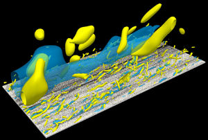
We show in figure 3 the axes (black lines) of vortices with sizes  $\sigma ^{+}=30$ and $240$. We see that the identified axes are located along the centre lines of yellow and red tubular objects, which are the positive isosurfaces of $Q^{(\sigma )}$. Thus the method can identify objectively the vortex axes without any threshold.

Figure 3. Axes of vortices at scales (a)  $\sigma ^{+}=30$ and (b) $\sigma ^{+}=240$. Transparent yellow and red objects are isosurfaces of the second invariant $Q^{(\sigma )}/Q^{(\sigma )}_{rms}=1$ of the velocity gradient tensor at the same scales. In (a), we visualize a subdomain (half in the streamwise and spanwise directions) of the computational domain.
Incidentally,  $\sigma ^{+}=30$ is of the order of the smallest-scale vortices ( $5\eta \lesssim \sigma \lesssim 20\eta$, with $\eta$ being the Kolmogorov scale), whereas $\sigma ^{+}=240$ is approximately the largest-scale vortices ( $\sigma \approx h/4$). Our previous study (Motoori & Goto Reference Motoori and Goto2021) examined turbulent channel flow at $Re_\tau =4179$ obtained by DNS of Lozano-Durán & Jiménez (Reference Lozano-Durán and Jiménez2014) to show that wall-attached ( $\sigma \approx y$) vortices are quasi-streamwise vortices, whereas wall-detached ( $\sigma < y$) vortices are distributed isotropically. These characteristics, which are indeed observed in figure 3, are important when we investigate particle clustering. In §§ 4.2 and 4.3, we use the identified axes to examine the spatial distribution of particles around vortices with four different sizes ( $\sigma ^{+}=30$, $60$,
$60$,  $120$ and $240$).
3.3. Streaks
We investigate in § 4.4 the aggregation of particles into the hierarchy of low-speed streaks. For this purpose, we extract the spine (the centre line on the wall) of each streak. We identify lines composed of the local minima in the spanwise direction of  $u^{(\sigma )}$ at the grid point closest to the wall, i.e. the points satisfying
 \begin{equation} \frac{\partial u^{(\sigma)}}{\partial z} = 0\quad {\rm and}\quad u^{(\sigma)} < 0. \end{equation}
The black lines in figure 4 show the identified spines of streaks for the scales  $\sigma ^{+}=30$ and $240$. We see that they are located under streaks at each scale. Similar methods were used by many authors (e.g. Schoppa & Hussain Reference Schoppa and Hussain2002; Lee et al. Reference Lee, Lee, Choi and Sung2014; Lee, Sung & Zaki Reference Lee, Sung and Zaki2017; Kevin, Monty & Hutchins Reference Kevin, Monty and Hutchins2019).

Figure 4. Spines of low-speed streaks at scales (a)  $\sigma ^{+}=30$ and (b) $\sigma ^{+}=240$. Transparent blue objects are the negative isosurfaces of the streamwise fluctuating velocity (a) $u^{(\sigma )+}=-1.2$ and (b) $u^{(\sigma )+}=-0.6$ at the same scales. We visualize a subdomain (half in the wall-normal direction) of the computational domain.
4. Results
4.1. Spatial distribution of particles
We show in figure 5 the two-dimensional ( $y$–
$y$– $z$) spatial distributions of inertial particles with $St_+=10$, $25$,
$25$,  $100$ and $250$ in the statistically steady state. We visualize only particles in a thin ( $200$ wall units) layer. Particles with smaller $St_+$ values ( $St_+=10$ and $25$) form small voids and clusters, whereas for larger $St_+$ values ( $St_+=100$ and $250$), such smaller-size clustering is obscure. Instead, larger clusters are prominent for $St_+=100$ and $250$. This multiscale nature is verified quantitatively in figure 6 by the average pair correlation function (e.g. Landau & Lifshitz Reference Landau and Lifshitz1980; Kostinski & Shaw Reference Kostinski and Shaw2001; Chen, Goto & Vassilicos Reference Chen, Goto and Vassilicos2006)
 \begin{equation} {\mathcal{M}}=\frac{\langle (\delta n)^{2} \rangle_\ell}{\langle n \rangle_\ell^{2}} -\frac{1}{\langle n \rangle_\ell}, \end{equation}
where  $\langle n \rangle _\ell$ and $\langle (\delta n)^{2} \rangle _\ell$( $=\langle (n-\langle n \rangle _\ell )^{2} \rangle _\ell$) are, respectively, the average and variance of the number of particles in each box of size $\ell ^{3}$. If cluster size is sufficiently smaller than box size, then ${\mathcal {M}}$ becomes zero because $n$ obeys the Poisson distribution with $\langle (\delta n)^{2} \rangle _\ell = \langle n \rangle _\ell$. Therefore, ${\mathcal {M}}$ represents the size- $\ell$-dependent clustering degree. We can see in both panels in figure 6 that around $\ell ^{+}\approx 10$, ${\mathcal {M}}$ values for $St_+ = 10$ and $25$ (the second and third smallest circles) are larger than $St_+=100$ and $250$. This means that particles with $St_+ = 10$ and $25$ are more likely to form voids and clusters with size $\ell ^{+}\approx 10$ than $St_+=100$ and $250$. In contrast, around $\ell ^{+}\approx 100$, ${\mathcal {M}}$ for $St_+=100$ (the fifth smallest circles in the insets of figure 6) is larger than $St_+ = 10$ and $25$. These are consistent with the visualizations (figure 5). More precisely, comparing the results between figures 6(a) $200 \leq y^{+} < 600$ and 6(b) $600 \leq y^{+} < 1000$, farther away from the wall, particles with a given $St_+$ tend to create larger clusters. This multiscale clustering in the bulk region is similar to that in turbulence in a periodic cube (e.g. Yoshimoto & Goto Reference Yoshimoto and Goto2007).

Figure 5. Two-dimensional ( $y$–
$y$– $z$) spatial distributions of particles with (a) $St_+=10$, (b) $St_+=25$, (c) $St_+=100$, and (d) $St_+=250$, within a streamwise layer of thickness $200$ wall units.

Figure 6. Average pair correlation function of particles in the layers (a)  $200 \leq y^{+} < 600$ and (b) $600 \leq y^{+} < 1000$. From smaller (and darker) to larger (and lighter) circles, $St_+=1$, $10$,
$10$,  $25$,
$25$,  $50$,
$50$,  $100$, $250$ and $1000$. The insets show the close-up for the range $\ell ^{+} \geq 50$.
Comparing figures 5(b)  $St_+=25$ and 5(d) $250$, we notice that the numbers of particles in the bulk region are different. This is because particles with $St_+=25$ concentrate more near the walls through the turbophoresis. We show in figure 7 the average wall-normal concentration profile $c(y)$ in the statistically steady state, which is the ratio of the average number density of particles within a thin layer ( $4$ wall units) to the bulk number density. Here, the average is taken over time and the homogeneous directions. We see that particles with $St_+= 10$, $25$ and $50$ concentrate in the near-wall region. The observation is reasonable because these particles are carried by buffer-layer structures and trapped in the viscous sublayer ( $y^{+}\lesssim 5$) (Soldati & Marchioli Reference Soldati and Marchioli2009; Bernardini Reference Bernardini2014).

Figure 7. Average number density of particles as a function of height  $y^{+}$. From thinner (and darker) to thicker (and lighter) lines, $St_+=1$, $10$,
$10$,  $25$,
$25$,  $50$,
$50$,  $100$, $250$ and $1000$.
Since the Reynolds number is high enough, in addition to buffer-layer vortices, wall-attached larger-size vortices and wall-detached vortices co-exist (see figure 3). In the following two subsections, to understand the role of the multiscale vortices in the transport of particles, we investigate the relationship between the observed multiscale clusterings and the hierarchy of vortices.
4.2. Particle voids and the hierarchy of wall-detached vortices
To show quantitatively the origin of multiscale clusterings of particles, we use the identification of vortex axes introduced in § 3.2. This enables us to evaluate the number of particles around the axis of each coherent vortex. In this subsection, we show the results for wall-detached vortices, i.e. vortices whose size  $\sigma$ is smaller than their existing height ( $\sigma < y$). Since the vortex axes are distributed isotropically (Motoori & Goto Reference Motoori and Goto2021), we evaluate the number density $N_{p|vor}$ of particles as a function of the distance $r$ from the vortex axes. For the conditional average, we set the bin width of $r$ as $\varDelta _{bin}=\sigma /6$.
We first show, in figure 8(a),  $N_{p|vor}(r)$ around the axes of the small-size ( $\sigma ^{+}=30$; see figure 3a) vortices existing in the layer $200\leq y^{+}<400$. The thinner (and darker) lines show the results for particles with smaller Stokes numbers. Since we have confirmed that $N_{p|vor}(r)$ is almost constant for $r \geq 3\sigma$ (i.e. particles are homogeneous for $r \geq 3\sigma$), we normalize the values by those at $r=3\sigma$. Looking at the second thinnest line ( $St_+=10$), we see that the number density takes the minimum at $r=0$, whereas it takes the maximum around $\sigma \lesssim r\lesssim 2\sigma$. This tendency is also observed for particles with Stokes numbers (e.g. $St_+=1$ and $25$) close to $St_+=10$. In contrast, the number density of particles with $St_+\gtrsim 100$ is almost constant, irrespective of $r$. Hence in the layer $200 \leq y^{+}< 400$, the small-size vortices are more likely to sweep out particles with $St_+\approx 10$.

Figure 8. Average number density of particles existing at distance  $r$ from an axis of vortices with sizes (a,b) $\sigma ^{+}=30$ and (c) $\sigma ^{+}=240$, in layers (a) $200\leq y^{+}<400$ and (b,c) $800\leq y^{+}<1000$. The values are normalized by that at $r=3\sigma$. From thinner (and darker) to thicker (and lighter) lines, $St_+=1$, $10$,
$10$,  $25$,
$25$,  $50$,
$50$,  $100$, $250$ and $1000$. In (d), we show $N_{p|vor}(0)$, which is indicated by the arrows in the other panels: (a) yellow open triangles, (b) yellow closed triangles, and (c) red closed triangles, as functions of $St_+$.
Next, looking at the results for vortices with  $\sigma ^{+}=30$ for the higher height $800\leq y^{+} <1000$ (figure 8b), we can see that the vortices sweep out predominantly particles of $St_+=25$. We replot in figure 8(d) the values at $r=0$ with yellow triangles, which are indicated by the arrows in figures 8(a,b), as functions of $St_+$. It is clear that vortices with the same size but at different heights do not necessarily contribute to creating voids of particles with the same relaxation time.
Figure 8(c) shows  $N_{p|vor}$ around vortices with a large size ( $\sigma ^{+}=240$) within the layer $800\leq y^{+}< 1000$( $=h^{+}$). The results are for particles around the heads ( $y \approx h$) of quasi-streamwise vortices (see figure 3b), and we call them wall-detached vortices in the sense that $\sigma < y$. We see in figure 8(c) that particles with $St_+=100$ are swept out most significantly, and they form clusters around the vortices ( $r\approx \sigma$). Red triangles in figure 8(d) show $N_{p|vor}(0)$ as a function of $St_+$ indicated by the arrow in figure 8(c). Comparing the three lines, vortices with different sizes and heights create voids of particles with different $St_+$.
In addition to figure 8(d), we plot in figure 9(a)  $N_{p|vor}(0)$ for vortices at the fixed size $\sigma ^{+}=30$ in four different layers. We also show in figure 9(b) the results for the vortices with four different sizes ( $\sigma ^{+}=30$, $60$,
$60$,  $120$ and $240$) in the fixed layer $800\leq y^{+}< 1000$. These two panels show that for larger sizes or farther distance from the wall (shown by the lighter lines), the vortices tend to sweep out particles with larger $St_+$. Note that the well of each line shifts to larger $St_+$. This implies that vortices sweep out particles of the relaxation time comparable with their turnover time. To verify this quantitatively, we define the time scale $\tau _{Q}=1/\sqrt {Q_{rms}^{(\sigma )}}$ of vortices in terms of the root-mean-square value $Q_{rms}^{(\sigma )}(y)$ of the second invariant of the velocity gradient tensor at scale $\sigma$. Note that the time scale is a function of $y$ and $\sigma$. We then define the local Stokes number by
 \begin{equation} St_Q(\sigma,y)=\frac{\tau_p}{\tau_{Q}(\sigma,y)}. \end{equation}
The quantities shown in figures 9(c) and 9(d) are the same as in figures 9(a,b) but as functions of  $St_Q$ instead of $St_+$. Here, we have used the value of $\tau _Q$ at the centre in each layer. We see that the minimum of the curve collapses around $St_Q\approx 0.2$. We can therefore conclude that, irrespective of the existing height and size, vortices preferentially sweep out particles of the relaxation time $\tau _p$ comparable with the turnover time $\tau _Q$. This observation around wall-detached vortices is similar to that in homogeneous turbulence (Bec et al. Reference Bec, Biferale, Cencini, Lanotte, Musacchio and Toschi2007; Yoshimoto & Goto Reference Yoshimoto and Goto2007; Wang et al. Reference Wang, Wan, Yang, Wang and Chen2020b; Oka & Goto Reference Oka and Goto2021). The importance of the time scale matching was also pointed out by Soldati & Marchioli (Reference Soldati and Marchioli2009) for the clustering in the buffer layer in low-Reynolds-number turbulence.

Figure 9. Average number density of particles existing in the region ( $0\leq r<\varDelta _{bin}$, where $\varDelta _{bin}=\sigma /6$) near an axis of (a,c) vortices with fixed size $\sigma ^{+}=30$ in the different layers $200\leq y^{+}<400$ (black), $400\leq y^{+}<600$ (dark grey), $600\leq y^{+}<800$ (light grey) and $800\leq y^{+}<1000$ (very light grey), and (b,d) vortices with the different sizes $\sigma ^{+}=30$ (black grey), $\sigma ^{+}=60$ (dark grey), $\sigma ^{+}=120$ (light grey) and $\sigma ^{+}=240$ (very light grey) in the fixed layer $800\leq y^{+}<1000$. The values are functions of (a,b) $St_+$, and (c,d) $St_Q$.
The Kolmogorov second similarity hypothesis gives the time scale  $\tau _v$ of vortices with size $\sigma$ in the inertial range as
 \begin{equation} \tau_v^{+}(\sigma,y) \sim{(\sigma^{+})}^{{2}/{3}}{(\epsilon^{+})}^{-({1}/{3})}. \end{equation}
Here,  $\epsilon$ is the mean energy dissipation rate. For turbulent channel flow, if we assume equilibrium between the energy dissipation $\epsilon$ and the energy production, the log law of the mean velocity profile and $-\overline {\check {u}\check {v}}^{+}\approx 1$ in the log layer (Rotta Reference Rotta1962), then the energy dissipation rate is estimated by
 \begin{equation} \epsilon^{+}\sim{-}\overline{\check{u}\check{v}}^{+}\,\frac{\partial U^{+}}{\partial y^{+}} \approx(\kappa y^{+})^{{-}1}.\end{equation}
Therefore, we can rewrite (4.3) as
 \begin{equation} \tau_v^{+}(\sigma,y)\sim {(\sigma^{+})}^{{2}/{3}}{(y^{+})}^{{1}/{3}}. \end{equation}
We have evaluated in figures 9(c,d) the turnover time of the vortices with size  $\sigma$ and at height $y$ in terms of $\tau _Q$. We show in figure 10(a) that $\tau _{Q}$ obeys the scaling (4.5) in the inertial range in the log layer. The thinner (and darker) grey lines indicate the time scale of smaller-size vortices, and the blue dashed lines with the same thickness indicate $\tau _v$ (see (4.5)) for the same $\sigma$. Looking at the thinnest grey and blue lines ( $\sigma ^{+}=30$), we see that they are overlapped for $60 \lesssim y^{+} \lesssim 200$. For $y^{+}\gtrsim 200$, where the lines do not overlap, the scale $\sigma ^{+}=30$ is in the dissipation range ( $\sigma \lesssim 10\eta$). The two lines for $\sigma ^{+}=60$ are also in good agreement for $120 \lesssim y^{+} \lesssim 400$. Therefore, in the inertial range in the log layer (e.g. $10\eta \lesssim \sigma \lesssim y/2$), $\tau _{Q}$ obeys the scaling (4.5). Incidentally, the time scale $\tau _\omega = 1/\sqrt {\overline {\omega _i^{(\sigma )2}}}$ is similar to $\tau _Q$ (figure 10b), which might be easier to estimate.

Figure 10. Time scales evaluated by (a)  $\tau _Q$ and (b) $\tau _\omega$ of vortices with size $\sigma$ and height $y$. Note that in (b), we plot $2.5\tau _\omega ^{+}$ to fit the blue dashed lines: $\tau _v^{+} = C{(\sigma ^{+})}^{{2}/{3}} {(y^{+})}^{{1}/{3}}$ with $C = 0.9$. From thinner (and darker) to thicker (and lighter) lines, $\sigma ^{+}=30$, $60$,
$60$,  $120$ and $240$.
We summarize the results in this subsection. In turbulent channel flow, wall-detached vortices ( $\sigma < y$) most effectively sweep out particles of the relaxation time comparable with their turnover time irrespective of their size (figure 9d) and their existing height (figure 9c). Hence the origin of the multiscale voids is the hierarchy of vortices, and we can explain the multiscale nature in terms of time scale matching between particles and vortices. We may use the scale-decomposed velocity gradients (e.g. enstrophy and the second invariant of the velocity gradient tensor) to estimate the turnover times of vortices (figure 10). In the next subsection, to show the importance of the time scale matching for wall-attached vortices ( $\sigma =y$), we examine particle clustering around quasi-streamwise vortices with various sizes.
4.3. Particle voids and the hierarchy of wall-attached vortices
In order to investigate multiscale voids and clusters created by the hierarchy of wall-attached quasi-streamwise vortices, we show the two-dimensional ( $y$–
$y$– $z$) distribution of particles around quasi-streamwise vortices. First, we show results for quasi-streamwise vortices with positive streamwise vorticity in the buffer layer. Figures 11(a–c) show the conditionally averaged number density – more precisely, the number density of particles around the axes of vortices rotating clockwise at $\sigma ^{+}=30$ and $y^{+}=30$. The values are normalized by the average number density at each height. We see in figure 11(a) that the number of particles with $St_+=10$ is smaller around the vortex core (black closed circle). In contrast, the particles form a cluster in the left region in the panel, where strong ejection is induced by the vortices. This means that in the buffer layer ( $y^{+}\approx 30$), quasi-streamwise vortices (with size $\sigma ^{+}\approx 30$) sweep out particles with $St_+=10$ from their cores, and the nearby ejection carries particles away from the wall. As a result, the particles form clusters in low-speed streaks. In other words, the creation mechanism of particle voids is the same as that by wall-detached vortices (§ 4.2), whereas the formed clusters are inhomogeneous in the spanwise direction due to a nearby low-speed streak. This result implies that the clustering mechanism in terms of coherent structures described by Soldati & Marchioli (Reference Soldati and Marchioli2009) holds in the buffer layer irrespective of the Reynolds number. The clustering degree becomes weaker for particles with longer relaxation times $St_+=25$ (figure 11b) and $St_+=100$ (figure 11c).

Figure 11. Average number density of particles with (a,d)  $St_+=10$, (b,e) $St_+=25$, and (c, f) $St_+=100$, in the $y$–
$y$– $z$ plane around an axis (black closed circle) of quasi-streamwise vortices with sizes (a–c) $\sigma ^{+}=30$ and (d–f) $\sigma ^{+}=240$, with positive streamwise vorticity (clockwise rotation). The values are non-dimensionalized by the average number density at each height.
Next, figures 11(d–f) show results for quasi-streamwise vortices with a larger size  $\sigma ^{+}=240$. In contrast to the results for buffer-layer-size vortices, the channel-half-width-size vortices more predominantly sweep out the particles with $St_+=100$ (figure 11f) than $St_+=10$ (figure 11d). We also show in figure 12 the number density on the axis (black closed circle) for $\sigma ^{+}=30$, $60$,
$60$,  $120$ and $240$ as functions of $St_+$ and $St_Q$. We observe that the values take the minimum around $St_Q\approx 0.2$ irrespective of the size of vortices. This observation is the same as that for wall-detached vortices (figure 9). We therefore conclude that, irrespective of the size, existing height and type (wall-detached or wall-attached) vortices, the time scale matching is the key to the creation of multiscale voids in high-Reynolds-number wall turbulence.

Figure 12. Average number density of particles existing in the region ( $y=\sigma$ and $z=0$) on an axis of quasi-streamwise vortices with sizes $\sigma ^{+}=30$ (black), $\sigma ^{+}=60$ (dark grey), $\sigma ^{+}=120$ (light grey) and $\sigma ^{+}=240$ (very light grey) at height $y=\sigma$ as functions of (a) $St_+$ and (b) $St_Q$.
We emphasize that the results for wall-attached vortices are consistent with the previous study (Bernardini Reference Bernardini2014) on the wall-deposition process of particles in turbulent channel flow. Particles with  $St_+\approx 10$ are swept out from quasi-streamwise vortices in the buffer layer (figure 11a), whereas larger-size vortices hardly sweep out these particles (figure 11c). This implies that even if the Reynolds number increases – that is, the number of the levels in the hierarchy of wall-attached vortices increases – such larger-size vortices do not contribute to the transport of particles with $St_+ \approx 10$ from and to the wall. This is the reason why the wall-deposition process (i.e. the so-called diffusional deposition mechanism) of particles with $St_+\approx 10$ is universal irrespective of the Reynolds number, as was shown by Bernardini (Reference Bernardini2014). In contrast, large-size quasi-streamwise vortices can transport particles with larger $St_+$ ( $\gtrsim 100$, figure 11f). This is also consistent with the fact shown by Bernardini (Reference Bernardini2014) that the wall-deposition rates of particles with $St_+ \gtrsim 100$ are determined by the Stokes number $St_o=\tau _p u_\tau /h$ defined by the turbulent time scale in the outer layer (i.e. the so-called free-flight mechanism).
As was mentioned above, clusters formed by wall-attached vortices tend to be formed in the ejections. This means that particles swept out by quasi-streamwise vortices are likely to be accumulated in low-speed streaks. We indeed observe the multiscale attraction into the streaks in figure 13, which shows the two-dimensional ( $x$–
$x$– $z$) spatial distributions of particles with $St_+=10$ and $250$. Particles for larger $St_+$ form larger-size streamwise-elongated clusters. In the next subsection, we investigate further the multiscale attraction mechanism of particles by low-speed streaks with different sizes.

Figure 13. Two-dimensional ( $x$–
$x$– $z$) spatial distributions of particles with (a) $St_+=10$ and (b) $St_+=250$, within $0< y^{+}<50$.
4.4. Particle clusters and the hierarchy of streaks
To verify quantitatively that multiscale low-speed streaks contribute to the attraction of particles, we show the average number density  $N_{p|low}$ in the $y$–
$y$– $z$ plane around spines of low-speed streaks. The identification method has been introduced in § 3.3.
We show, in figures 14(a–c),  $N_{p|low}$ around low-speed streaks at scale $\sigma ^{+}=30$. The number density is normalized by the average at each height. The number of particles with $St_+=10$ (figure 14a) is larger in the region around the white closed circle ( $y=\sigma$ and $z=0$). This implies that the particles are likely to concentrate in low-speed streaks. It is also important that the trend is weaker for particles with longer relaxation times $St_+=100$ (figure 14b) and $St_+=1000$ (figure 14c). In contrast, we see in figures 14(d–f) that low-speed streaks with a larger size ( $\sigma ^{+}=240$) attract particles with longer relaxation times $St_+=100$ (figure 14e) and $St_+=1000$ (figure 14f).

Figure 14. Average number density of particles with (a,d)  $St_+=10$, (b,e) $St_+=100$ and (c, f) $St_+=1000$, in the $y$–
$y$– $z$ plane around a spine of the low-speed streak at the sizes (a–c) $\sigma ^{+}=30$ and (d–f) $\sigma ^{+}=240$. The values are non-dimensionalized by the average number density at each height.
Moreover, we show in figure 15(a) the values at the centre (white closed circle) of the low-speed streaks as functions of  $St_+$. Lighter lines show the results for larger sizes ( $\sigma ^{+}=30$, $60$,
$60$,  $120$ and $240$). As expected from figure 14, larger-size streaks contribute to the attraction of particles of larger $St_+$ into their centre. Figure 15(b) shows the same quantities as in figure 15(a) but as functions of the local Stokes number $St_Q$ (see (4.2)). The number of the particles takes the maximum in a range $0.2 \lesssim St_Q \lesssim 2$ irrespective of the size of streaks. Therefore, we conclude that the hierarchy of low-speed streaks attracts particles of the relaxation time comparable with the turnover time of accompanying quasi-streamwise vortices. In other words, at each level of the hierarchy, particles are swept out from quasi-streamwise vortices (§ 4.3), and they form clusters in a nearby low-speed streak.

Figure 15. Average number density of particles existing in the region ( $y=\sigma$ and $z=0$) on a spine of low-speed streaks with sizes $\sigma ^{+}=30$ (black), $\sigma ^{+}=60$ (dark grey), $\sigma ^{+}=120$ (light grey) and $\sigma ^{+}=240$ (very light grey), at the height $y=\sigma$ as functions of (a) $St_+$ and (b) $St_Q$.
Before closing this subsection, it is worth mentioning that the clusters formed by smaller-size streaks are much more prominent (figure 14), although this is not clear in the visualizations (figure 13). This observation is consistent with the result that smaller-size quasi-streamwise vortices tend to form stronger clusters (figure 12). This is because smaller-size wall-attached vortices (i.e. those in the buffer layer) are more likely to carry particles from the viscous sublayer, where particles concentrate most (see figure 7), to the bulk.
5. Discussions
5.1. Description of multiscale clustering in terms of multiscale vortices
We have shown that the time scale matching between particles and vortices is most important to explain multiscale clustering. In this subsection, we demonstrate that a simple argument based on the equations of motion leads to the same conclusion. For this purpose, we introduce imaginary particles (Oka & Goto Reference Oka and Goto2021) that obey
 \begin{equation} \frac{{{\rm d}} {\boldsymbol{x}_p^{*}}}{{{\rm d}} {t}} = \boldsymbol{u}_p^{*} \end{equation}
and
 \begin{equation} \frac{{{\rm d}} {\boldsymbol{u}_p^{*}}}{{{\rm d}} {t}} ={-}\frac{1}{\tau_p}\,(\boldsymbol{u}_p^{*}-\boldsymbol{u}^{(\sigma)_{low}}) . \end{equation}
Here,  $\boldsymbol {x}_p^{*}$ and $\boldsymbol {u}_p^{*}$ are the position and velocity of the imaginary particles, respectively, and $\boldsymbol {u}^{(\sigma )_{low}}$ is the velocity field coarse-grained at the scale $\sigma$ (see (3.1)). The imaginary particles are affected only by velocity larger than $\sigma$. This model is consistent with the present results (e.g. figures 5 and 8) that larger-scale clusters are formed around larger-scale vortices. Therefore, it is reasonable to assume that the clusters of real particles governed by (2.1) are similar to those of imaginary particles governed by (5.1). Incidentally, by simulating the imaginary particles in periodic turbulence, our previous studies (Oka & Goto Reference Oka and Goto2021; Oka, Watanabe & Goto Reference Oka, Watanabe and Goto2021) verified this assumption numerically. Here, we extend this argument to wall turbulence.
First, by applying the argument of Maxey (Reference Maxey1987) to (5.1), we express the relative velocity of particles to fluid as
 \begin{equation} \boldsymbol{u}_p^{*}-\boldsymbol{u}^{(\sigma)_{low}} \approx{-}\tau_p \boldsymbol{a}^{(\sigma)_{low}}. \end{equation}
Here,  $\boldsymbol {a}^{(\sigma )_{low}}$ is the coarse-grained acceleration of fluid. Note that (5.2) yields under the condition that $\tau _p$ is sufficiently smaller than $T(\sigma ;y)$, where $T(\sigma ;y)$ is the eddy turnover time for size $\sigma$ and height $y$. As shown in figure 10, since we estimate $T$ by $\tau _Q$, (5.2) holds for $\tau _p \lesssim \tau _Q(\sigma ;y)$. Then, taking the divergence of (5.2), we obtain
 \begin{equation} {-}{\boldsymbol{\nabla}\boldsymbol{\cdot}{\boldsymbol{u}_p^{*}}}\approx \tau_p (\boldsymbol{\nabla}\boldsymbol{\cdot}{\boldsymbol{a}^{(\sigma)_{low}}}). \end{equation}
The left-hand side implies the accumulation rate  $\gamma$( $=-\boldsymbol {\nabla }\boldsymbol {\cdot }{\boldsymbol {u}_p^{*}}$) of the particles when considering them as a continuum. In other words, the particles accumulate in the region satisfying $\gamma > 0$, whereas the particles are swept out from the region satisfying $\gamma < 0$. In the inertial range, since the acceleration is approximated by the pressure gradient (i.e. $\boldsymbol {a}^{(\sigma )_{low}}\approx -({1}/{\rho _f})\,\boldsymbol {\nabla }{p^{(\sigma )_{low}}}$), we can rewrite (5.3) as
 \begin{equation} -{\boldsymbol{\nabla}\boldsymbol{\cdot}{\boldsymbol{u}_p^{*}}}\approx{-}\tau_p \left(\frac{1}{\rho_f}\,\nabla^{2} p^{(\sigma)_{low}}\right) ={-}\tau_p Q^{(\sigma)_{low}}. \end{equation}
Hence the accumulation rate is determined by  $Q^{(\sigma )_{low}}$, that is, particles are swept out from rotational regions ( $Q^{(\sigma )_{low}}>0$), whereas they accumulate in irrotational regions ( $Q^{(\sigma )_{low}}<0$). Moreover, if we estimate $Q^{(\sigma )_{low}}$ by ${\tau _Q}^{-2}$, then we can evaluate the order of the clustering time $T_{cluster}$( $=1/\gamma$) as
 \begin{equation} T_{cluster}\approx \frac{\tau_Q^{2}(\sigma,y)}{\tau_p}. \end{equation}
It takes  $T_{cluster}$ for particles with $\tau _p$ to be swept out from vortices with the turnover time $\tau _Q(\sigma,y)$. If $T_{cluster}$ is shorter than the lifetime $T_{life}$ of vortices, then the particles are swept out completely. Therefore, a necessary condition for forming voids and clusters is given by
 \begin{equation} T_{cluster} \lesssim T_{life}\quad\Longleftrightarrow\quad \frac{\tau_Q^{2}(\sigma, y)}{T_{life}(\sigma, y)} \lesssim \tau_p. \end{equation}
Next, recall that (5.2) holds under the condition  $\tau _p \lesssim \tau _Q(\sigma,y)$. We then obtain the clustering condition
 \begin{equation} \frac{\tau_Q^{2}(\sigma, y)}{T_{life}(\sigma, y)}\lesssim \tau_p \lesssim \tau_Q(\sigma,y) . \end{equation}
Vortices with eddy turnover time  $\tau _Q$ and lifetime $T_{life}$ sweep out effectively particles with relaxation time $\tau _p$ satisfying condition (5.7). If we assume that $T_{life}$ is proportional to $\tau _Q$, then we conclude that vortices are most likely to sweep out particles with $\tau _p\approx \tau _Q$. This is the reason why the local Stokes number $St_Q$( $=\tau _p/\tau _Q$) is important for the clustering condition. Recall that in the inertial range of the log layer, the scaling $\tau _Q \sim \sigma ^{{2}/{3}}y^{{1}/{3}}$ holds (see § 4.2). Therefore, we can predict that particles with a given relaxation time $\tau _p$ at height $y$ are swept out from vortices with size $\sigma \sim \tau _p^{{3}/{2}}y^{-({1}/{2})}$. We emphasize that the scaling is also valid for much higher Reynolds number wall-turbulence because there is a wide range of the log layer. Incidentally, under the assumption $T_{life} \approx \tau _Q$, since the clustering time (see (5.5)) is estimated as $T_{cluster} \approx \tau _Q$( $\approx \tau _p$), larger vortices take longer time to form particle clusters. This is consistent with the results by Liu et al. (Reference Liu, Shen, Zamansky and Coletti2020) that the lifetime of the clusters is also longer for larger ones.
Furthermore, it is worth mentioning that since it takes a finite time to sweep out particles, the created voids can be located in different regions from present vortices. This history effect is important especially in streamwise inhomogeneous turbulence (e.g. adverse-pressure-gradient turbulent boundary layers).
5.2. Particle velocity statistics
The above results and discussions suggest that the hierarchy of coherent structures plays an important role in transporting inertial particles. By using this, in the present subsection, we explain the particle velocity statistics, which determine the wall-normal distribution of particles (such as shown in figure 7), in terms of the scale-dependent fluid velocity.
As described in detail by Johnson et al. (Reference Johnson, Bassenne and Moin2020), if we assume that the particle Reynolds number is sufficiently small (i.e. when the Stokes drag coefficient  $k_p$ in (2.1b) is unity), then the wall-normal concentration $c(y)$ of particles in the statistically steady state is written as
 \begin{equation} c(y)=\frac{\mathcal{N}}{\langle v_p^{2}\,|\,y \rangle} \exp\left(\frac{1}{\tau_p}\int^{y} \frac{\langle v\,|\,\xi \rangle}{\langle v_p^{2}\,|\,\xi \rangle}\,{{\mathrm{d}}} \xi\right). \end{equation}
Here,  $\mathcal {N}$ is an integration constant, and $\langle \cdot \,|\,y \rangle$ denotes the average sampled by the position of particles $y=y_p$; namely, $\langle v_p^{2}\,|\,y \rangle$ is the variance of the wall-normal particle velocity, and $\langle v\,|\,y \rangle$ is the mean wall-normal fluid velocity at $y=y_p$. If the relaxation time of particles is sufficiently large ( $\tau _p^{-1} \to 0$), we can approximate (5.8) as
 \begin{equation} c(y)\approx \frac{\mathcal{N}}{\langle v_p^{2}\,|\,y \rangle}. \end{equation}
This implies that  $\langle v_p^{2}|y \rangle$ determines the concentration of particles for larger $St_+$. Johnson et al. (Reference Johnson, Bassenne and Moin2020) showed that (5.9) is a good approximation for $St_+\gtrsim 128$ in low-Reynolds-number turbulent channel flow ( $Re_\tau =150$).
As has been discussed in the previous subsection (§ 5.1), we consider the imaginary particles that obey (5.1). Since the relative velocity of particles to fluid is expressed by (5.2) under the condition  $\tau _p \ll T(\sigma ;y)$, we can approximate $\langle v_p^{2}\,|\,y \rangle$ as
 \begin{equation} \langle v_p^{2}\,|\,y \rangle\approx \langle (v^{(\sigma)_{low}}-\tau_p a_y^{(\sigma)_{low}})^{2}\,|\,y \rangle\approx \langle v^{(\sigma)_{low}2}\,|\,y \rangle. \end{equation}
In addition to this approximation in the zeroth order of  $\tau _p$, if we assume homogeneity (i.e. $\langle v^{(\sigma )_{low}2} \rangle \approx \langle v^{(\sigma )_{low}2}\,|\,y \rangle$), then we can estimate $\langle v_p^{2}\,|\,y \rangle$ in terms of the scale-dependent fluid information of $\langle v^{(\sigma )_{low}2} \rangle$. Here, we choose the filter scale $\sigma$ so that it satisfies $T(\sigma ;y) = \tau _p$, where $T$ is expressed by
 \begin{align}T&=C\sigma^{{2}/{3}}y^{{1}/{3}}\quad \mathrm{if}\ y \geq 2\sigma, \end{align}
 \begin{align}T & =2^{{1}/{3}}C\sigma \qquad \, \mathrm{if}\ y < 2\sigma,\end{align}
with  $C=0.9$. This expression is based on the results shown in figure 10.
We show in figures 16(a,b) the left- and right-hand sides of (5.10), respectively; that is, figure 16(a) shows the variance  $\langle v_p^{2}\,|\,y \rangle$ of the wall-normal velocity of particles with $St_+=25$, $50$,
$50$,  $100$, $250$ and $1000$, and figure 16(b) shows the variance $\langle v^{(\sigma )_{low}2} \rangle$ of wall-normal fluid velocity coarse-grained at different scales $\sigma (\tau _p;y)$ satisfying $T(\sigma ;y)=\tau _p$. It is clear that these two quantities for $St_+=25\text {--}100$ behave in a similar manner, which implies that (5.10) gives a good approximation. We therefore conclude that we can describe the variance $\langle v_p^{2}\,|\,y \rangle$ of particle velocity in terms of $\langle v^{(\sigma )_{low}2} \rangle$ by choosing $\sigma$ that satisfies $T(\sigma ;y) = \tau _p$. More concretely, for $y \gtrsim 2\sigma$, the ratio between these quantities is almost constant. This means that (5.11a) is a good expression for the time scale of wall-detached vortices. In contrast, for $y \lesssim 2\sigma$, $\langle v_p^{2}\,|\,y \rangle$ is larger than $\langle v^{(\sigma )_{low}2} \rangle$. This is because the transport of particles for $y \ll \sigma$ is determined by other factors, for example, the foot ( $y \ll \sigma$) of wall-attached vortices. However, it is hard to quantify their effects from the scale-decomposed turbulent fields obtained by the present coarse-graining method. Note that we do not show $\langle v^{(\sigma )_{low}2} \rangle$ for $St_+=1$ and $10$ in figure 16, since the corresponding filter scale $\sigma$ is smaller than the grid width.

Figure 16. (a) Variance of the wall-normal particle fluctuating velocity. (b) Variance of the wall-normal fluid velocity at scales  $\sigma (\tau _p;y)$ satisfying $T=\tau _p$, where $T$ is expressed by (5.11). From thinner (and darker) to thicker lines, $St_+=25$, $50$,
$50$,  $100$, $250$ and $1000$.
Incidentally, to predict the wall-normal concentration  $c(y)$ (see (5.8)) of particles by using $\langle v^{(\sigma )_{low}2} \rangle$, we need to take into account the effect of the viscous sublayer, where particles concentrate most (see figure 7). Moreover, when the Stokes number is small, the approximation (5.9) is invalid, and $\langle v\,|\,y \rangle$ is another factor determining the concentration (see (5.8)). These detailed studies are left for a future study. Furthermore, although we have employed the assumption of perfectly elastic collisions between particles and solid walls, in a more realistic situation, this assumption is invalid (Joseph et al. Reference Joseph, Zenit, Hunt and Rosenwinkel2001; Gondret et al. Reference Gondret, Lance and Petit2002). The difference in the restitution coefficient may affect the concentration profile.
6. Conclusions
To investigate the transport mechanism of inertial particles in high-Reynolds-number turbulent channel flow, we have conducted DNS of those with seven relaxation times ( $St_+=1$, $10$,
$10$,  $25$,
$25$,  $50$,
$50$,  $100$, $250$ and $1000$) in turbulence at $Re_\tau =1000$. The key ingredient of our analysis is the objective identification of the hierarchy of coherent flow structures (§ 3). By using this, we have shown the average distribution of particles around the axes of vortices (§§ 4.2 and 4.3) and around the spines of streaks (§ 4.4) at each level of the hierarchy. The analyses lead to revealing the role of coherent structures in the multiscale clusterings of particles. Vortices create particle voids with the size of themselves by sweeping out particles of the relaxation time comparable with their turnover time. This mechanism holds irrespective of the size, existing height and type (wall-detached or wall-attached) of vortices. Hence the multiscale clusterings are determined by the local Stokes numbers ( $St_Q\approx 0.2$) at any level of the hierarchy of vortices (figures 9c,d). We have also shown that particles swept out by wall-detached tubular vortices form clusters isotropically around them, whereas those swept out by wall-attached vortices are attracted by a nearby low-speed streak (figures 12b and 15b). Particles swept out by smaller-size wall-attached vortices form denser clusters (figures 11, 12 and 15) because smaller-size (buffer-layer-size) vortices carry particles from the wall. In § 5.1, extending the arguments (Oka & Goto Reference Oka and Goto2021; Oka et al. Reference Oka, Watanabe and Goto2021) of particle clustering in periodic turbulence to wall turbulence, we have also demonstrated that the above clustering mechanism is explained in terms of the imaginary particles advected by the filtered velocity. We have also explained the velocity statistics and concentration profile of inertial particles in terms of the hierarchy of coherent flow structures (§ 5.2).
Funding
This study was partly supported by the JSPS Grants-in-Aid for Scientific Research 20H02068 and 21K20403. The DNS were conducted under the auspices of the NIFS Collaboration Research Programs (NIFS20KNSS145) and under the supercomputer Fugaku provided by RIKEN through the HPCI System Research projects (hp200273 and hp210207).
Declaration of interests
The authors report no conflict of interest.


 Open access