


Introduction
The stability of the marine West Antarctic ice sheet in response to global climate change is a matter of some concern (Reference HughesHughes, 1973; Reference WeertmanWeertman, 1974; Reference Thomas and BentleyThomas and Bentley, 1978; Reference Thomas, Sanderson and RoseThomas and others, 1979; Reference BindschadlerBindschadler, 1991). In the “Ross embayment,” the drainage of the ice sheet is into the Ross Ice Shelf, mostly through a suite of five ice streams (A, B, C, D and E). Understanding the dynamics of these ice streams and the region around them is the key to understanding the stability of the ice sheet.
Radar sounding has been used extensively to profile the surface and bed of the inland ice of the “Ross embayment” (Reference Robin, Evans, Drewry, Harrison and PetrieRobin and others, 1970; Reference HughesHughes, 1973; Reference RoseRose, 1979; Reference DrewryDrewry, 1983; Reference Shabtaie and BentleyShabtaie and Bentley 1987, Reference Shabtaie and Bentley1988; Reference Shabtaie, Whillans and BentleyShabtaie and others, 1987). Flight lines for those soundings, however, were widely (50–100 km) and/or irregularly spaced. During the 1988–89 field season of the Siple Coast Project, we collected 14 000 km of airborneradar data along a grid of flight lines regularly spaced 510 km apart, over the upstream parts of Ice Streams A, Β and C (Fig. 1). In this paper, we discuss the collection, reduction and interpretation of these data, which have resulted in the most accurate and detailed surface elevation, ice thickness and bed topography to date in the area they cover. The maps of surface topography and ice thickness in the papers by Reference Shabtaie, Whillans and BentleyShabtaie and others (1987) and Reference Shabtaie and BentleyShabtaie and Bentley (1988), respectively, remain the best for the downstream parts of the ice streams; they also extend slightly farther upstream above Ice Streams B1 and B2 than our study does.

Fig. 1. Map of the Siple Coast Project study region showing the outline of the 1988–89 airborne-radar coverage. Flights covered six blocks: a, b, c, e, 10 block and 20 block. The ice streams and UpB and UpC camps (heavy solid circles) are labeled. Surface stations of the Siple Coast Project (solid circles), Ross Ice Shelf Geophysical and Glaciological Survey (open circles), and the IGY Ross Ice Shelf traverse (open squares) are shown. Grounding lines are shown by short-dashed lines. The long-dashed line is the boundary between confluent Ice Streams B1 and B2. The base map is from Reference Shabtaie and BentleyShabtaie and Bentley (1988). The origin of the rectangular grid coordinate system used on this and subsequent maps is at the South Pole; grid north is toward Greenwich and therefore toward the top of the map. Squares have sides of length equal to 1° of latitude along the 180° meridian..
In our maps, we use a rectangular grid system that provides the same sense of compass directions (e.g. grid north towards the top, grid east towards the right) as a Mercator projection at lower latitudes. Use of a single grid system for areal and regional maps means that they will have the same orientation as a properly oriented map of Antarctica as a whole. Our grid coordinates are defined simply by a polar-to-rectangular coordinate conversion: grid latitude = (90°−L)cosλ; grid longitude = (90°−L) sin λ, where L and λ are the geographic south latitude and east longitude, respectively. Negative grid coordinates mean grid southerly latitudes and grid westerly longitudes.
Radar System
The radar system used was a modified SPRI Mark IV 50 MHz radar (Reference Schultz, Powell and BentleySchultz and others, 1987) mounted in a DeHavilland Twin Otter aircraft. The data were digitized using a LeCroy 3500 SA data-acquisition system and stored on an Exabyte EXB-8200 8 mm videocassette. The antenna system consisted of two folded dipoles encased in airfoil-shaped housings, and mounted ![]() wavelength (1.5 m) under the wings of the Twin Otter (Reference Shabtaie and BentleyShabtaie and Bentley, 1987). The radar returns were monitored during collection using both a Biosonics Model Ν 115 portable chart recorder and a Tektronix 2465 300 MHz oscilloscope.
wavelength (1.5 m) under the wings of the Twin Otter (Reference Shabtaie and BentleyShabtaie and Bentley, 1987). The radar returns were monitored during collection using both a Biosonics Model Ν 115 portable chart recorder and a Tektronix 2465 300 MHz oscilloscope.
The aircraft was equipped with a Litton LTN92 inertial-navigation system (INS), a Sperry model 200 radar altimeter and a Rosemount pressure transducer. Communication between these various aircraft sensors and the data-acquisition system was provided by an Airtech Aviation DAI-800 data-acquisition interface system.
The radar system transmits a 300 ns pulse with a peak envelope power of 750 W at a pulse repetition rate of 750 pulses s−1 Every 2 s, an individual trace is extracted and recorded as a raw trace (“raw” refers to a trace that has not been stacked with adjacent traces).
Synchronously, 512 traces, continuously stored into a data buffer, are summed together and recorded as a stacked trace.
Survey-Grid Design and Data Collection
Five blocks (a, b, c, 10 and 20) (Fig. 2) were flown in both the transverse (perpendicular to stream flow) and longitudinal (parallel to ice-stream flow) directions. One block (e), far from the base camp, could only be flown transversely owing to logistic constraints. The 14000 km of airborne-radar profiling were collected during 24 4 h flights.
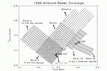
Fig. 2. A map of the six blocks showing all transects, The Ohio State University satellite-surveyed ground stations ( small crosses), The Ohio State University strain grid on Ice Stream C (solid rectangle), and UpB and UpC camps (heavy solid circles).
Most surface features of the ice sheet have a characteristic length scale of 10 km or greater. The surface is generally smooth with few abrupt changes — typical surface slopes range between 0.002 and 0.005. Most major features of the bed topography also exceed 10 km in width, although the bed is, of course, much rougher than the surface — slopes commonly exceed 0.05. To sample the bottom features adequately, flight lines spaced 5 km apart would have been desirable. Due to logistical constraints, however, this was possible only near the UpC base camp (block b) and in specific areas where dense coverage was necessary (blocks 10 and 20, which coincide with photogrammetric blocks of The Ohio State University). A 10 km line spacing was used elsewhere.
The aircraft was flown at a constant-pressure elevation (normally between 500 and 1000 m). The horizontal and vertical positioning of the aircraft were determined from its INS and pressure altimeter, respectively. In addition, the height-above-terrain measurement from the radar altimeter was recorded. The controling computer supplied time calibration.
At an average air speed of 60 ms−1 (120 kt), a raw and a stacked trace were recorded every 120 m. Individual traces were sampled using quadrature sampling (Reference Taner, Koehler and SheriffTaner and others, 1979). Sampling at a carrier-frequency phase lag of 270° (the digitizer is too slow to sample at a lag of 90°) gave an effective sampling interval of 40 ns (twice the period of the carrier).
Data Reduction
The data consist of approximately 150000 traces with a total data volume of approximately 650 megabytes. Many procedures had to be developed to reduce this large data set to a format in which the reflections could be picked and ultimately maps created. The computer code required to achieve this goal was developed by Geophysical and Polar Research Center technical staff and graduate students, both present and former (more details are available upon request).
Sample data and auto-picker
Three dominant signals can be seen on a sample transect (Fig. 3): (1) the transmit pulse, which serves as the time reference; (2) the reflected return from the surface of the ice; and (3) the echo from the ice-bedrock interface. In general, the bottom reflection is strong and easily detected, although at times the ice gets too thick or the bed too rough and the bottom reflection is lost. Noise between the surface and bottom reflections is mainly scatter from buried and exposed surface crevasses, or poorly resolved internal layers.
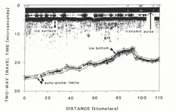
Fig. 3. A sample transect from block b. The transmit pulse, surface refection and bottom reflection are shown. Noise from surface and near-surface diffractions appears between the surface and bottom refection. The numbered triangles along the top border are event marks recorded when flying over a surface feature or a ground station of known location. The user-set limits of the auto-picker are shown above and below the bottom refection as open squares connected by a line. A two-way travel time in ice of 1 s corresponds to about 85 m.
To create maps from these data, the onset time of the surface and bottom reflection must be “picked” (determined). The large volume of data precluded picking onset times manually, so an interactive, “mouse”-driven computer routine to pick onset times was developed. The auto-picker works by selecting the sample (MAXPOS) with maximum amplitude (MAXVAL) (Fig. 4) between limits defined by the operator (Fig. 3). It then selects the maximum slope between the upper limit and MAXPOS. This slope is extrapolated back to zero amplitude and the onset time (ONSETPOS) is recorded. If ONSETPOS is outside the limits of the auto-picker, the pick is undefined. The r.m.s. amplitude between LIMITI and ONSETPOS is called NOISE. The r.m.s. sample amplitude between ONSETPOS and MAXPOS is called SIG + NOISE. The signal/noise (S/ N) ratio is then calculated using:
For each trace, ONSETPOS, MAXPOS, MAXVAL and S/N are recorded. We have found that this auto-picker routine works on traces with S/N ratios as low as 2: 1.

Fig. 4. Cartoon of a sample pulse between the user-set limits of the auto-picker. The various parameters solved for are labeled and their relation to the pulse shape is shown. The horizontal axis is time, the vertical axis is signal amplitude.
Converting travel time to ice thickness
Ice thicknesses were calculated from the difference between basal and surficial reflection times using an average velocity for electromagnetic waves in ice of 171 m μs−1. This is the same velocity used by Reference Shabtaie and BentleyShabtaie and Bentley (1988) when creating similar maps in West Antarctica. Using an average velocity of 171 m μs−1 is equivalent (for ice 1000 m thick) to using a velocity in solid ice of 169 m μs−1 and adding 10 m to correct for low-density firn (cf. Reference Shabtaie and BentleyShabtaie and Bentley, 1988). Thicknesses greater than 1000 m will be slightly exaggerated by this procedure; the error is 20 m at an ice thickness of 2500 m, the thickest our system is capable of penetrating. We have not attempted to discriminate between reflection hyperbolae and real bottom echoes; no migration corrections have been applied.
Converting pressure-transducer readings
The height of the aircraft above the surface must be resolved to establish a surface elevation. Calculating the height requires converting the reading of the pressure transducer to meters above a reference level using (Reference Ostenso and BentleyOstenso and Bentley, 1959):

where Z0 is the reference elevation (600 m at UpC), Κ is the barometric constant (18400 m), B0 is the reference pressure (920 mbar at UpC), Β is the observed pressure, a is the coefficient of thermal expansion of air (0.00367 Κ−1), θ is the mean temperature of the air column between Ζ and Z0, ϕ is the latitude of observation point, and k and k′ are constants that depend on the gravity field of the Earth. (We used k = 0.0052884, k′ = 0.0000059 from the International Gravity Formula; substitution of a more modern gravity model would have a negligible effect on our results.)
The temperature gradient in the air column was accounted for by using the first data point in the transect as a reference (Zref ) and assigning it the default temperature θ of −10° C. At successive points, a temperature difference (δt) is calculated using the elevation difference (Z – Zref ) and an assumed vertical temperature gradient (tgrad) of −1° C (100 m)−1 as
Then, the new average air-column temperature correction is applied to the previously calculated elevation (Zold)
These corrections are negligible (<1 m) for most of the data set, yet at times, when the aircraft more than doubled its elevation to avoid cloud cover, the correction could be as much as 10 m. The elevation of the ice surface was usually calculated by subtracting the radar-altimeter reading from the aircraft height. Exceptions are discussed in the next section.
Missing data
On eight transects, all data acquired from aircraft sensors by the Airtech DAI-800 data-acquisition interface system were lost because of a recurring instrumental-connection problem. Loss of the pressure-transducer readings made it impossible to resolve the surface elevation for these transects. However, data were recorded from the radar-sounding system for these eight transects and ice thicknesses were measured. The horizontal position of the aircraft was determined by linear interpolation between the starting and ending coordinates for each transect.
On one transect, the aircraft elevation exceeded the range of the pressure transducer (800 mbar), resulting in the loss of surface-elevation measurements. The radar-altimeter data were lost for 12 transects, partly from instrumental problems and partly from flying at an elevation that exceeded the range of the radar altimeter. Picking the onset time for the transmit pulse and surface reflection of the sounding radar provided an alternative method of determining surface elevation for these transects.
Throughout the survey, glitches comprising one or two absent records in an otherwise complete and continuous recording occurred in the data stream from the Airtech DAI-800 data-acquisition system. A simple linear interpolation based on a least-squares straight-line fit to the five nearest data points was used to fill in the missing points. The changes in values (x-y position, pressure, radar altimeter, etc.) over such a short interval are very small, so linear interpolation should suffice.
Larger gaps occurred in the output of the auto-picker when the S/N ratio was small and undefined picks resulted. In these cases the gaps were filled by fitting a second-order polynomial to the surrounding points by least squares. However, rather than minimizing the squares of the residuals, ri
, the quantities ![]() were minimized. The weighting function has the form
were minimized. The weighting function has the form
where wi
is the S/N ratio for the ith record along the interval, and ![]() is the distance of the ith record from the center point. Weighting by this factor has the effect of emphasizing the effect of high S/N records and records near the gap relative to low S/N records and records farther from the gap. The number of adjacent points used in the smoothing depended on the average S/N ratio of the points in question (additional points were included until the sum of
is the distance of the ith record from the center point. Weighting by this factor has the effect of emphasizing the effect of high S/N records and records near the gap relative to low S/N records and records farther from the gap. The number of adjacent points used in the smoothing depended on the average S/N ratio of the points in question (additional points were included until the sum of ![]() for those points was greater than five times the average S/N ratio of the transect as a whole.)
for those points was greater than five times the average S/N ratio of the transect as a whole.)
Navigation
A major obstacle to obtaining an accurate horizontal position of each data point is the drift in the INS of the aircraft. The 22 flight closures for the whole survey have a mean of 2.0 km and a standard deviation of 0.97 km, with a maximum closure of 3.7 km. Navigational errors of a kilometer or two are also indicated by the positions recorded when passing over satellite-surveyed ground stations. (The instant of nearest approach, as estimated by an observer in the aircraft, was electronically marked on the data stream by pushing a button, thereby producing an “event mark”.) The nature of INS drift is not well understood. After analysis of the flight closures and the relation between event marks and ground stations, it was decided that the best approach was to assume a linear drift with time. Corrections were applied on this basis, using the closure at the end of each flight.
Cross-over analysis
In two-dimensional coverage, each transverse transect within a block crosses each longitudinal transect (see Fig. 2) at a cross-over point. Since all data contain error, the calculated value of surface elevation or ice thickness from one line at the cross-over point differs from that of the other line. The value and spatial distribution of these differences, the cross-over errors, provide insight into the magnitude and source of the error in the data.
The cross-over errors for ice thickness and surface elevation were used first to evaluate the effectiveness of the linear-drift correction for navigation. The standard deviation (σ) in ice-thickness cross-over errors for block b was reduced from 36 m before the drift correction to 25 m after. For surface elevation, the corresponding reduction was from 4.5 m to 3.7 m. A reduction in σ of about 20% is typical of the effect on all blocks and shows that applying a linear-drift correction to the navigation improves the accuracy of the data.
A major complication in obtaining surface elevations is the fact that atmospheric pressure changes with time, which in turn affects the indicated height of the aircraft. Each survey block consists of several different flights that were not necessarily flown on the same day. Figure 5a shows a histogram of the surface-elevation cross-over errors for block c. The effect of a several mbar (several hundred Pascal) pressure change during data collection is seen in the bimodal distribution, which indicates that one part of the block is artificially higher than the other part.

Fig. 5. Surface-elevation cross-over errors for block c (a) before and (b) after least-squares minimization.
Linear-inverse theory (Reference MenkeMenke, 1984) was used to minimize the surface-elevation cross-over errors in a least-squares sense. The model parameters calculated were the vertical shifts of each transect; for simplicity, the vertical shift is assumed constant for each transect. (Numerical experiments showed that more complex adjustment schemes, such as shifts linear in space and/or time, while conceptually more satisfying, did not improve results significantly.) Let
δli ≡ height correction to the ith longitudinal transect, i = 1 to n;
δtj ≡ height correction to the jth transverse transect, j = 1 to m;
lij ≡ indicated surface-elevation value on the ith longitudinal transect where the jth transverse transect crosses it;
tij ≡ indicated surface-elevation value on the j transverse transect where the ith longitudinal transect crosses it;
Δij ≡ tij is the cross-over error where the ith longitudinal transect crosses the jth transverse transect.
We minimize the cross-over errors by solving the overdetermined linear-matrix equation Gm = d where

The column matrices d and m have Ν = nm and M = n + m elements, respectively, and G is an appropriate Ν × M matrix of elements 0, 1 and −1. The least-squares minimization condition is satisfied by solving the equation GTGm = GTd for m.
The solution is subject to an arbitrary constant (i.e. a vertical shift of the entire surface) which we fix by applying the arbitrary constraint ∑mi = 0, where mi are the elements of m (This constraint is not physically required since there is no reason to believe that the summation of the shifts should equal zero. It is simply an intermediate step to give a definite solution; we later adjust the overall level of the surface to fit independent measurements of surface elevation.) The constraint is a linear equality of the form Fm = h and is implemented using the method of Lagrange multipliers (Reference MenkeMenke, 1984, sect. 3.10). This method results in the simultaneous solution of two equations, put in matrix form as follows

where λ is the Lagrange multiplier.
Figure 5b shows the surface-elevation cross-over errors for block c after the minimization process. The bimodal distribution has been removed and the errors have been reduced greatly. This method worked equally well for all other bidirectional blocks, although the magnitudes of the pre-minimization errors varied.
Zeroing remanent cross-over errors
After the above processing, cross-over errors still remained that had to be removed to avoid ambiguity in the gridding and contouring routines. This was done by linear distribution of the errors, as follows.
For each transect segment between two cross-points there are two corresponding cross-over errors, e1 and e2 one at each end of the segment. The data values (surface elevations or ice thicknesses) along the segment were then adjusted according to
where ds is the adjusted data value, d the unadjusted value, x the distance along the segment from the first cross-point, and L the length of the segment. This adjustment was applied to both surface elevation and ice thickness.
Interpolation
In order to contour these data, they had to be interpolated from their dense distribution along widely spaced transects to an evenly spaced grid. Every eighth “stacked” data point was used, resulting in a data point approximately every 960 m along a transect. The “Surfer” Version 4 software package (Golden Software Inc., Golden, Colorado) was used to interpolate and contour the data. The interpolation was performed using a procedure called Kriging (Reference OleaOlea, 1974, Reference Olea1975; Reference DavisDavis, 1986). Kriging was chosen after a comparison with the other two interpolation methods available in “Surfer” (minimum curvature and inverse distance) showed that Kriging produced the smoothest contour lines and tended best to enhance the trends of topographic features. The procedure makes use of the semi-variogram (plot of semi-variance vs distance between points (Reference OleaOlea, 1977)) of the data to find the optimal set of weights to apply to the surrounding data points when estimating the surface elevation or ice thickness at unsampled locations. Points within a search radius of 0.2° were used to calculate the elevation estimates. “Surfer” uses a linear form of the semi-variogram; from sample semi-variograms created from the data, we decided that the linear model approximates the true form of the semi-variogram closely enough that we did not need to use a more complex form.
These data were gridded at a density of one grid point every 1.11 km (0.01° of latitude). This is appropriately less dense than the 960 m spacing of the ungridded data along the transects. No smoothing was performed on the data after they were gridded. A standard contouring routine was applied to the gridded data to produce elevation and ice-thickness maps.
Ties to ground stations
To eliminate the uncertainty in surface elevations that arises from the fact that they are all based on the barometric altimeter in the aircraft, they were tied to ground stations of known elevation. The ground control for our survey comprised satellite-surveyed stations of an Ohio State University network (personal communication from I. M. Reference Whillans and van der VeenWhillans, 1990). Stations exist in all six of our survey blocks, although the number and distribution vary from block to block. Elevations at these stations relative to the WGS-72 ellipsoid were determined by Transit satellite tracking to an accuracy of ± 2 m. The elevations were then referred to the Rapp Set A geoid model distributed by the Magnavox Corporation to purchasers of their “Geoceivers” under a cover marked “GEM-IOC”. The same geoid was used as the reference for maps of surface elevation produced by Reference Shabtaie and BentleyShabtaie and Bentley (1987) and Reference Shabtaie, Whillans and BentleyShabtaie and others (1987) and mistakenly identified by them as GEM-10C.
The tie was accomplished using the residuals between the ground-station elevations and the mapped elevation at those locations. As a first step, the elevations in each block were uniformly raised or lowered to bring the mean of the residuals for that block to zero. The elevation residuals remaining after these shifts still show a trend across each block that arises from lateral gradients in atmospheric pressure (see Figure 6 for an example). An additional correction therefore was made by allowing the surface to tilt, using a planar fit to each block to minimize the residuals. The validity of the tilting procedure was verified by three different results. (1) The residuals between the ground stations and the grid were greatly reduced, by as much as 50% for some blocks. (2) Fits at common boundaries between different blocks were improved. (3) Many small depressions initially present on the surface-elevation maps opened up into continuous linear valleys, which are more commonly seen on an ice sheet.

Fig. 6. Block 10 showing ground-station residuals (m) after the gridded block was shifted vertically to remove the mean of the residuals but before the tilt correction was applied. Ground stations are marked by small crosses and UpB by a heavy solid circle. The dashed line marks the axis between more positive residuals (top) and more negative residuals (bottom) around which the grid plane was tilted.
Maps
The corrected data were combined into data sets that included all six blocks and maps were created of surface elevation (Fig. 7), ice thickness (Fig. 8) and (by taking the difference between surface elevation and ice thickness) bed topography (Fig. 9). The contour intervals are 20, 100 and 100 m, respectively. These contour intervals satisfy the principle that 90% of the errors should fall within half the contour interval (2σ criterion; Reference Davis and McCullaghDavis and McCullagh, 1975). This limits the likely distortion of the contours by noise. Nevertheless, features delineated by only one contour line should be treated with caution. In particular, the many small circles and ovals that lie on only one flight line surely do not depict the real topography or thickness accurately. Also, small distortions of individual contour lines in Figure 7 could make open features out of closed ones (e.g. the closed minimum just above and to the left of the letters “B2”).

Fig. 7. Surface-elevation map with a contour interval of 20 m. The borders of the ice streams are shown by heavy solid lines. “RAB” and “RBC” are Ridge AB and Ridge BC, respectively. Data points are shown along transects as small dots.

Fig. 8. Ice-thickness map with a contour interval of 100 m. The borders of the ice streams are shown by heavy solid lines. “RAB” and “RBC” are Ridge AB and Ridge BC, respectively. Data points are shown along transects as small dots.

Fig. 9. Bottom-topography map. Contours are in depths below sea level with a contour interval of 100 m. The borders of the ice streams are shown by heavy solid lines. “RAB” and “RBC” are Ridge AB and Ridge BC, respectively. Data points are shown along transects as small dots.
The ice-stream boundaries shown in Figures 7–9 are from Reference Shabtaie and BentleyShabtaie and Bentley (1988), mapped primarily on the basis of heavy crevassing as evinced by strong radar back-scatter (“clutter”). For an updated version of the boundaries of Ice Streams B1 and B2, the reader should refer to Reference Whillans and van der VeenWhillans and Van der Veen (1993).
Error Analysis
Error estimates from individual sources
The outgoing radar pulse expands spherically and is only weakly focused. Therefore, the reflection recorded from a sloping reflector is from the point, upslope from the nadir point, that is closest to the source, so the vertical distance to the reflector is underestimated (Reference Brenner, Bindschadler, Thomas and ZwallyBrenner and others, 1983). This “migration error” is totally negligible (![]() ) for reflections from the ice surface but not for reflections from the bed. Furthermore, refraction at the air–ice interface creates a wave front that is no longer spherical in the ice (Reference Brown, Rasmussen and MeierBrown and others, 1986). Calculations using an aircraft height of 500–1000 m (as in our survey) showed that refraction at the air-ice interface causes an additional 30–50% increase in the migration error for soundings. The error is also a function of the slope of the bed of the ice sheet. The average bed slope of all the grids was estimated at 0.03, for which the migration error is 1.5 m. In the roughest areas, where the bed slope is as great as 0.07, the migration error is about 8 m.
) for reflections from the ice surface but not for reflections from the bed. Furthermore, refraction at the air–ice interface creates a wave front that is no longer spherical in the ice (Reference Brown, Rasmussen and MeierBrown and others, 1986). Calculations using an aircraft height of 500–1000 m (as in our survey) showed that refraction at the air-ice interface causes an additional 30–50% increase in the migration error for soundings. The error is also a function of the slope of the bed of the ice sheet. The average bed slope of all the grids was estimated at 0.03, for which the migration error is 1.5 m. In the roughest areas, where the bed slope is as great as 0.07, the migration error is about 8 m.
Errors in the horizontal positioning of the aircraft due to INS drift result in errors in the elevation estimate of both the surface and bottom topography. The INS drift contains two components, a linear component and an oscillating component called the Schuier drift (Reference Hodge, Wright, Bradley and JacobeHodge and others, 1990). Following Reference Hodge, Wright, Bradley and JacobeHodge and others (1990), we assumed that the linear-drift correction (discussed earlier) corrects for the linear component and that the standard deviation of all the closure errors represents the magnitude of the Schuier component. The standard deviation then reflects a random sampling of the Schuier component. Using the standard deviation of the flight closures (0.97 km) and combining with a resolution error of 200 m for the resolution of the INS gives an estimated navigation error of 1.0 km, a value we assumed during the remaining analysis.
The error in the elevation estimate is β α, where β is the vector navigation error and α is the vector slope of the surface or ice bottom. Thus, for the surface elevations, with an average slope of ∼0.004, the average error is 4.0 m; for the ice-bottom elevations, with an average slope of ∼0.03, it is 30 m.
The pressure transducer has an estimated relative accuracy of 0.5 mbar, i.e. about 4.5 m in height. The cross-over analysis (discussed earlier) removes temporal pressure variations. Ties to ground stations remove spatial pressure variations to the extent that they fit the planar model applied. The remaining errors should be small compared to errors from other sources.
The radar altimeter is accurate to better than 1 m. The lower frequency of the sounding radar and the picking error (next paragraph) for both the transmitted pulse and the reflection gives a higher error for surface elevations determined from the sounding radar (∼2.5 m). The sounding radar had to be used for surface elevations on only 8% of the transects, so 1 m was used as the overall instrumental standard error.
Any inaccuracy in the pick of the onset time by the auto-picker results in an error in the estimate of surface elevation or ice thickness. Where the S/N ratio is ≥2: 1, as in the surface reflection, the auto-picker can pick the onset time to half a sample interval or 1.7 m. The quality of the reflection from the ice bottom, however, is influenced by several factors: (1) the amount of scattering at the air-ice interface, (2) the thickness of the ice and the spreading loss, (3) the roughness of the bed of the ice sheet, and (4) the dielectric contrast between the ice and the material immediately below the ice. All of these factors therefore affect the accuracy of the auto-picker. An examination of many picked records led us to estimate the average picking error for the ice-bottom reflection of 7 m.
The grid points located between transects are subject to interpolation errors. The accuracy of the gridding method depends on the smoothness of the surface in question and the density of coverage. Surface slopes can be correlated easily over the 5 or 10 km between transects; from examination of the mapped contours, we estimate the interpolation error for surface elevations to be 1 m. The ice-sheet bed, however, is much rougher so ice-thickness interpolation errors will be much larger — for this we estimate a standard error of 40 m for all blocks except e. The sparse spacing of transects and the rough nature of the bed in block e combine to make the interpolation there particularly inaccurate, perhaps as large as one contour interval (100 m).
The wave speed of 169 m μs−1 in solid ice is accurate to ± 1.0 m μs−1 (Reference CloughClough and Bentley, 1970; Reference RobinRobin, 1975; Reference Jezek and RoelofTsJezek and Roeloffs, 1983), which corresponds to an error in the ice thickness of 8.5 m in 1500 m of ice. The additional error that arises from the uncertainty in the correction for the low-density firn we estimate at 5 m.
The error estimates discussed above were combined (root sum square) to yield error estimates of 6 m and 52 m for surface elevation and ice thickness, respectively. The error estimate for the bottom elevations is essentially the same as for ice thickness.
Error estimates from cross-overs and ground stations
Two other methods exist for estimating the errors in surface elevations: cross-over analysis and ties to ground stations. The number of cross-over points and ground stations, and the root-mean-square cross-over residual for each type of comparison (after minimization of cross-over differences) are listed in Table 1. The agreement between the two types of error estimates, both overall and in their variation from block to block, is remarkable.
Table 1. Standard deviations of residuals at cross-over points and ground stations

The standard deviation of the residuals in blocks c and e are larger than those of the other blocks. There are several reasons for this. For block c: flight closures were not available for two of the flights, so navigational drift corrections could not be applied; the radar-altimeter data were lost on four transects so the less accurate radar-sounder reflection had to be used; the aircraft was flown too low on two transects, causing the surface reflection to be partially obscured by the tail of the transmit pulse; and surface elevations are completely missing for two longitudinal transects. For block e: the surface-elevation datum for each transect was based on only one crossover point with block c, owing to the lack of any longitudinal transects; the absence of longitudinal transects reduced the density of coverage and thus increased the interpolation error.
The average residuals for blocks a, b, 10 and 20 are 3.1 and 3.6 m for cross-overs and ground stations, respectively. This is considerably less than the standard-error estimate (interpolation excluded) of 6 m in the previous section, which suggests that the error analysis in that section was overly conservative. For blocks c and e, the surface-elevation error estimates are 6 m and 9 m, respectively.
The average cross-over residual for the ice thickness in blocks a, b, 10 and 20 is 27 m. This is close to the error estimate (interpolation excluded) of 32 m found in the previous section. The standard-error estimates for blocks c and e are 58 m and 35 m, respectively.
A direct measurement of the ice thickness has been made at only one location within the area mapped. Several holes were drilled through the ice sheet at UpB camp on Ice Stream Β (Reference Engelhardt, Humphrey, Kamb and FahnestockEngelhardt and others, 1990); measured ice thicknesses ranged from 1030 to 1058 m. Our survey indicates an ice thickness at UpB of 1064 m; the difference is well within the estimated error of the data set.
Discussion of the Maps
The maps contain a wealth of information about the ice sheet and its bed. We will comment on several aspects that we found particularly interesting.
-
1. In more places than not, surface slopes change little at the edges of the ice streams, either as shown in Figure 7 or as mapped by Reference Whillans and van der VeenWhillans and Van der Veen (1993). Only the downstream parts of the margins of Ice Stream B2 and the extension of the grid southern margin along Ice Stream Β could be delineated from the surface topography alone. Furthermore, in the case of the “Dragon” (the grid northern margin of Ice Stream B2), at least, the surface topography appears to reflect the asymmetric subglacial ridge that delineates that boundary, so any effect of change from ridge-flow to stream-flow is obscured.
-
2. The beds of Ice Streams B2 and Β are much smoother than those of Ice Streams A, B1 and C, at least in the parts mapped here (Fig. 9). (The beds of Ice Streams A and C also get smoother farther downstream (Reference Shabtaie and BentleyShabtaie and Bentley, 1988).) Elsewhere there is little noticeable difference in subglacial topography between the ice streams and the interstream ridges. The highest subglacial relief, in fact, underlies Ice Stream A. A trough does underlie part of Ice Stream B1 (grid 4.3° S, 4.2° W), but so does an adjacent ridge (Fig. 9). Farther upstream, the grid northeastern margin of the ice stream, as mapped, cuts across the trough, although control on the position of the margin is weak here (cf. Reference Shabtaie and BentleyShabtaie and Bentley, 1987, Fig. 2). The trough appears to be more coincidental than controling.
-
3. There are no striking differences on any of the maps between stagnant Ice Stream C and the rest of the mapped region (except Ice Streams B2 and B, as already noted above). The only suggestion of a different character for Ice Stream C is a more frequent occurrence than on the other ice streams of relative maxima in the surface elevations (closed contours in Figure 1).
-
4. The surface topography of the active ice streams is influenced little by the subglacial topography. This is most striking on Ice Stream A (the contours of surface topography in Figure 1 would probably be less regular if there had been longitudinal flight-line coverage, but the mapped character of the slope could not be grossly wrong); it is clear on Ice Stream B1.
-
5. The characteristics of the region described above strongly suggest that neither the bed topography nor the driving stress (proportional to the product of the surface slope and ice thickness) is the controling factor on the ice-stream existence. This confirms the conclusion drawn by Reference Shabtaie, Whillans and BentleyShabtaie and others (1987) from their reconnaissance survey. The control must come from some combination of the non-topographic nature of the bed (e.g. water pressure, dcformability, etc.) and the internal characteristics of the ice sheet.
-
6. The region we mapped extends far enough inland to be likely to include the transition zone from sheet flow to streaming flow in Ice Streams B1 and B2. A relatively steep slope that marks a drop in elevation of 100 m in 10 km does appear at the head of Ice Stream B1 (grid 3.9° S, 4.5° W), but an ice-stream-like velocity of 168 m a−1 exists another 10 km upstream (Reference Whillans and van der VeenWhillans and Van der Veen, 1993). A similar slope appears upstream from the beginning of the mapped boundaries of Ice Stream B2 (grid 4.6° S, 5.5° W), but the feature does not continue around the head of the ice stream and it probably simply reflects the subglacial ridge directly beneath it. Besides these two slopes, no other feature of any of the maps suggests a transition zone.
-
7. Going upstream on Ice Stream C, the regional surface slope gradually changes direction from along the axis of the ice stream to an angle of about 45° across-stream toward Ice Stream B2. At first, this suggests that, when Ice Stream C stagnated, ice far upstream that once flowed into Ice Stream C was diverted toward Ice Stream B2. However, it is not clear that the ice in this area (grid 4.6° S, 6.9° W) actually will flow into Ice Stream B2 across the broad intervening region of low and irregular slope. The fall line actually curves back, on the flank of a broad, low ridge (grid 4.3° S, 6.4° W to 4.8° S, 6.3° W), into Ice Stream C. That makes problematic the concept of the capture of the Ice Stream C catchment by Ice Stream B. Since Ice Stream C is far from a state of mass balance (Reference Whillans and van der VeenWhillans and Van der Veen, 1993), this ambiguity probably arises from ongoing changes in the flow regime. Analysis of the burial depth of crevasses suggests that the uppermost part of Ice Stream C has been the most recent to stagnate and that part of it even may still be active (Reference Retzlaff and BentleyRetzlaff and Bentley, 1993).
-
8. Closer to Ice Stream B, the regional surface slopes show clearly the convergence of ice into that ice stream. The contours form a broad arc from the edge of Ice Stream C to the middle of Ridge AB. There is no suggested flow laterally toward Ice Stream C and little toward Ice Stream A. It appears that almost all of the ice sheet between Ice Streams A and C flow into Ice Stream B.
Summary
Over 14000 km of high-quality digital airborne-radar data were collected over the upstream parts of Ice Streams A, Β and C in six gridded blocks with line spacings of 5–20 km. An automated and interactive processing procedure was developed for the reduction of these data. Cross-over analysis was implemented, as a constrained linear least-squares inverse problem, to remove the effects of temporal variations in atmospheric pressure. Interpolation of the data set to an evenly spaced grid was accomplished using the Kriging method. Surface elevations were fixed relative to the Rapp Set A geoid by tying the grids to satellite-surveyed ground stations, using a planar model fit.
Maps of surface elevation, ice thickness and bottom topography that show more detail than previous maps were produced. Standard-error estimates for the best-covered blocks were about 4 m for surface elevation, and about 30 m for ice thickness and bottom topography. For the more sparsely covered blocks the errors were larger: 6–9 m for surface elevation and 35–60 m for ice thickness.
We draw the following conclusions:
-
1. Neither the bed topography nor the driving stress controls where ice streams occur. Instead, the control must arise from the basal conditions and/or internal characteristics of the ice.
-
2. No geographic feature clearly demarcates a boundary between sheet flow and streaming flow anywhere within the mapped region.
-
3. The evidence concerning the putative capture of Ice Stream C by Ice Stream Β is ambiguous and leads to no clear conclusion.
-
4. Almost the entire ice sheet between Ice Stream A and Ice Stream C feeds into Ice Stream B.
Acknowledgements
The authors wish to thank the other members of the University of Wisconsin field party, C.G. Munson, A.N. Novick and, especially, S. Anandrakrishnan for their invaluable assistance in collecting the data. The Twin Otter aircraft was supplied, under contract from the U.S. National Science Foundation, by Ken Borek Air, Ltd, of Calgary. We are grateful for the high degree of cooperation shown by the Ken Borek Air crew. The comments of D.R. MacAyeal, I.M. Whillans and an anonymous referee resulted in significant improvements in this paper. This work was supported by U.S. National Science Foundation grant DPP86–14011. This is contribution No. 523 of the University of Wisconsin-Madison, Geophysical and Polar Research Center.
The accuracy of references in the text and in this list is the responsibility of the authors, to whom queries should be addressed.


