


1. Introduction
Concentrated vortices are fundamental flow features that are present in many important technical and natural flow fields. For example, strong concentrated vortices are formed at the tips of lifting surfaces (e.g. wings, control surfaces, rotor blades, wind turbines). These structures often interact with other vortices and/or with physical surfaces. The dynamics of these interactions is important to understand as it drives many processes that could be either beneficial (e.g. enhanced lift in dynamic stall) or detrimental (e.g. noise generation during blade vortex interaction in helicopter rotors) depending on the application. The interaction of a concentrated vortex core with a no-slip boundary has been shown to initiate flow along the axis of the vortex core (Kurosaka et al. Reference Kurosaka, Christiansen, Goodman, Tirres and Wohlman1988; Lundgren & Ashurst Reference Lundgren and Ashurst1989; Cohn & Koochesfahani Reference Cohn and Koochesfahani1993; Hagen & Kurosaka Reference Hagen and Kurosaka1993; Marshall & Krishnamoorthy Reference Marshall and Krishnamoorthy1997; Bohl & Koochesfahani Reference Bohl and Koochesfahani2004). This axial flow can become a dominant feature in the vortex dynamics and/or vortex–structure interaction.
Interest in flow fields with concentrated vortices containing axial flow is driven by several technical areas. For example, the passage of helicopter rotor blades creates concentrated trailing vortices behind the rotor blades. Following rotor blades can interact with the trailing vortex of the leading blade during forward flight, vertical descent and forward based descent. The resulting vortex–blade interaction is known to be a major source of helicopter noise. Understanding the dynamics of this interaction, and the effects on the vortical flow field, are critical to controlling and reducing helicopter noise (Conlisk Reference Conlisk1997) and in aerodynamic performance (Liu & Marshall Reference Liu and Marshall2004).
Classical solutions of rotational flow near a no-slip boundary have considered either a quiescent fluid above a rotating infinite plate (Kármán Reference Kármán1921), or solid body rotation over an infinite plate (Bödewadt Reference Bödewadt1940). These flows are illustrative in that the source of axial flow, or secondary flow, within the core of a vortex can be understood by examining these ‘simple’ flows.
Consider the case of solid body rotation of a fluid over a stationary plate. The flow has a constant angular velocity  $\omega$. Away from the wall, where the flow can be assumed inviscid, the $r$-momentum equation can be simplified to the Euler- $n$ equation, which for this flow equates the radial pressure gradient to the azimuthal velocity and radial location, R, as
 \begin{equation} \frac{\partial P}{\partial r}={-}\rho\frac{V^2_\theta}{R}. \end{equation}
Near the plate viscosity cannot be neglected. The azimuthal velocity,  $V_\theta$, is reduced but the radial pressure gradient is assumed to be the same as the far field via boundary layer approximations. The corresponding imbalance of forces indicates that fluid particles will move radially inward (for rotating fluid, fixed wall) near the wall and then away from the wall near the centre of rotation.
Solid body rotation, while illustrative, does not represent the vortical flow field of a concentrated line vortex. Past researchers (Rott & Lewellen Reference Rott and Lewellen1966; Burggraf, Stewartson & Belcher Reference Burggraf, Stewartson and Belcher1971) have sought similarity solutions for a generalized vortex, defined by the azimuthal velocity field,  $V_\theta \approx r^\alpha$, over a no-slip wall. The flow field of a generalized vortex is defined at the extremes by $\alpha = -1$ for a solid body rotation and $\alpha = +1$ for a potential vortex. Rott & Lewellen (Reference Rott and Lewellen1966) were limited to $\alpha < 0.1217$ because the solution diverged for larger values of $\alpha$. Burggraf et al. (Reference Burggraf, Stewartson and Belcher1971) were able to find solutions for the entire range of $\alpha$ by creating composite similarity solutions. Kuo (Reference Kuo1971) developed analytical solutions for vortices that simulated tornadoes, or flows in tornado chambers. The solution showed a strong upward motion of fluid within the core of the vortex and a weaker descending or recirculating motion outside the core region.
Koochesfahani (Reference Koochesfahani1989) investigated vortex shedding behind an oscillating NACA-0012 airfoil and observed that axial flow developed within the isolated vortex cores due to the interaction with solid no-slip boundaries (figure 1). Axial flow naturally develops at the test section wall (figure 1, plan view, outer dye traces), however, the boundary conditions at the outer wall are difficult to define due to the simultaneous formation of the vortices and the axial flow. The author placed a false wall in the flow field (approximately half-way down the plan view image at centre-span location) to investigate the axial flow for the fully developed vortices. The magnitude of axial flow speed was estimated, using dye flow visualization, from the displacement of dye and appeared to vary linearly (for constant oscillation amplitude) with the reduced frequency,  $k=({\rm \pi} cf)/U_\infty$, where c is the airfoil chord and f is the oscillation frequency. The magnitude of the axial flow velocity was found to be significant with respect to the free-stream velocity, ranging from 30 % to 65 % of free-stream speed, $U_\infty$. Bohl & Koochesfahani (Reference Bohl and Koochesfahani2004) quantified the axial flow speed in concentrated vortex cores due to interaction with the sidewalls of a water tunnel using single line tagging molecular tagging velocimetry (MTV) for similar conditions. Results showed that the peak axial flow speeds could be very high, of the order of the maximum swirl speed of the vortices. The maximum axial speed ratio (maximum axial speed normalized by maximum swirl speed) was found to vary in the range 0.6–1.0.

Figure 1. Side (centre-span) and plan view dye flow visualization of flow pattern of the concentrated vortex array in the wake of an oscillating airfoil. Panel (b) from Koochesfahani (Reference Koochesfahani1989).
Cohn & Koochesfahani (Reference Cohn and Koochesfahani1993) expanded on the work of Koochesfahani (Reference Koochesfahani1989) by investigating boundary conditions that initiate axial flow in a similar flow field using flow visualization. The authors investigated three distinct boundary conditions: no slip over an infinite length boundary, a finite length no-slip boundary and an enforced slip or ‘shear’ boundary. The results for the no-slip condition were consistent with the prior work. The finite length no-slip boundaries were comprised of airfoil-shaped streamline bodies and flat plates and covered a size range of  $2.6< L/R_0<380$, where $L$ was the length of the body that the vortex cores interacted with and $R_0$ was the radius of the vortex core. The results showed that axial flow was initiated with a flow structure qualitatively similar to the infinite length no-slip boundary. The shear boundary was created by placing an object in the flow upstream of the vortex array formation location. This created a wake boundary condition on the vortex array as it was formed. The result was a qualitatively different axial flow structure that was characterized by maximum axial flow at the edge of the vortex core and minimal axial flow in the centre of the core.
Quantitative studies in similar flow fields are limited. Laursen et al. (Reference Laursen, Rasmussen, Stenum and Snezhkin1997) investigated a vortex line pair formed by ejection through a slit into a still fluid using particle image velocimetry (PIV) and flow visualization. The results showed that, while the vortex pair was initially two-dimensional, it quickly broke up. Dye visualization showed the presence of strong axial flow with a core profile similar to what had been observed in prior work. The authors concluded that this axial flow was generated as a result of the viscous boundary condition at formation. The axial flow was not quantified in this work. Hirsa, Lopez & Kim (Reference Hirsa, Lopez and Kim2000) investigated the flow structure of a columnar vortex near a no-slip boundary. In this work, the columnar vortex was created via actuation of two flaps. The PIV was performed in a plane aligned with the axial direction of the vortex. The results showed inflow towards the vortex core near the wall. The authors observed a region of solid body rotation within the vortex core. In this region, the axial flow showed peaks on the outer edge of the vortex core with no axial flow in the centre of the vortex core. The axial flow profile in this region was similar to that observed by Cohn & Koochesfahani (Reference Cohn and Koochesfahani1993). This region was, however, spatially limited and the axial flow structure further away from the wall returned to a profile with a single peak located in the centre of the vortex core. The authors concluded that this recirculation region was a result of spatially oscillatory boundary layer structure associated with Bödewadt-type flows.
The work of Lundgren & Ashurst (Reference Lundgren and Ashurst1989) on the general behaviour of a vortex tube with a jet-like flow along its axis showed that the vortex supports the propagation of area-varying waves along its core. The propagation of these waves is governed by equations analogous to gas dynamics wave transport equations, with a wave ‘sound speed’ that scales linearly with the vortex circulation or its maximum swirl velocity. Vortex interaction with walls has been studied for vortices with and without axial flow already present (Krishnamoorthy & Marshall Reference Krishnamoorthy and Marshall1994; Marshall & Yalamanchili Reference Marshall and Yalamanchili1994; Marshall & Krishnamoorthy Reference Marshall and Krishnamoorthy1997; Liu & Marshall Reference Liu and Marshall2004). These studies show that cutting a vortex with axial flow present will produce either expansion or compression waves at the wall, depending on the direction of the axial flow with respect to the cutting wall. The area-varying waves travel along the core of the vortex away from the cutting surface.
There is generally limited quantitative experimental data available on the actual magnitude, spatial structure and evolution of the axial flow within the core of a well-characterized concentrated two-dimensional (2-D) line vortex that is cut by a thin solid plate. In particular, the time evolution of such data simultaneous with the measurements of vortex characteristics (e.g. core size, peak vorticity) is needed to understand the nature of the disturbance propagating along the vortex core and its possible relation to the area-varying waves predicted by Lundgren & Ashurst (Reference Lundgren and Ashurst1989).
The work described here considers the same flow geometry previously utilized by Bohl & Koochesfahani (Reference Bohl and Koochesfahani2004) and Bohl & Koochesfahani (Reference Bohl and Koochesfahani2009) to study the 2-D vortex array created in the wake of an oscillating airfoil. The appeal in using this geometry resides in the fact that a well-defined and well-characterized isolated vortex array with controllable properties can be generated by adjusting the oscillating airfoil control parameters. In the current study, as these 2-D vortices convect downstream they are cut by a thin plate that is placed at a prescribed downstream location, and the subsequent interactions are systematically investigated. The experiments are designed to operate in the regime of vortex cutting characterized by small thickness parameter (cutting plate thickness smaller than the vortex core radius) and high value of impact parameter (impact velocity of vortex approaching the cutting wall large enough compared with its maximum swirl velocity), as described in Marshall & Yalamanchili (Reference Marshall and Yalamanchili1994) and Marshall & Krishnamoorthy (Reference Marshall and Krishnamoorthy1997). Under these conditions, the experiments provide a good approximation to impulsive/instantaneous vortex cutting, where there is little vortex deformation before the vortex impact on the cutting wall and there is no boundary layer separation on the cutting wall prior to impingement. While we do provide data to characterize some of the changes that occur in the flow field at selected planes near the cutting wall surface due to vortex–wall interactions, the experiments are not designed to study the intricate dynamics of vortex interaction with the cutting wall boundary layer vorticity, the implications of which, in any case, do not impact the main conclusions made in this paper. Therefore, studying the disturbed boundary layer behaviour is outside the scope of this paper. Rather, the primary focus of this work is to investigate the existence of area-varying waves propagating along the vortex cores that are caused by the disturbances generated by vortex–wall interaction, and quantitatively assess their connection to the predictions of Lundgren & Ashurst (Reference Lundgren and Ashurst1989). To this end, the purpose of the current work is to: (i) simultaneously measure the axial flow characteristics and properties of the vortex, (ii) correlate those characteristics and (iii) investigate the possible presence and properties of travelling area-varying waves on the vortex cores predicted by Lundgren & Ashurst (Reference Lundgren and Ashurst1989).
2. Experimental set-up and methods
The experiments were conducted in a 10 000 l water tunnel (Engineering Laboratory Design, ELD) with a  $61\,{\rm cm} \times 61\,{\rm cm} \times 243\,{\rm cm}$ test section. A NACA-0012 airfoil with chord length $C = 12$ cm was placed in a flow with a free-stream velocity of $U_\infty = 10.5\,{\rm cm}\,{\rm s}^{-1}$, resulting in a chord Reynolds number $Re_c = 12\,600$. This Reynolds number was chosen to closely match the conditions of past work (Koochesfahani Reference Koochesfahani1989; Cohn & Koochesfahani Reference Cohn and Koochesfahani1993; Bohl & Koochesfahani Reference Bohl and Koochesfahani2009). For the work described here, the airfoil was oscillated sinusoidally about its 1/4- $C$ axis with an amplitude of $2^\circ$ and frequencies in the range $f= 1.45\unicode{x2013}3.21\,{\rm Hz}$. This corresponded to a variation of the reduced frequency of $k = 5.2\unicode{x2013}11.5$. The reduced frequency served as the control parameter and allowed the vortex properties such as circulation and peak vorticity to be varied.
Axial flow within the vortex cores naturally develops along the sidewalls of the tunnel, as shown in figure 1. In order to provide well-defined boundary conditions, two acrylic cutting walls (surface oriented in the  $x$–
$x$– $y$ plane) were placed into the flow with their leading edges located 6 cm ( $C/2$, $15r_{c,i}$) downstream of the airfoil trailing, and separated by a gap of $\pm$9.5 cm ( ${\pm }24r_{c,i}$) about the tunnel centreline, figure 2. The variable $r_{c,i}$ refers to the initial core radius of the 2-D concentrated line vortices approaching perpendicular to the cutting wall, which was nominally constant at $r_{c,i}\approx 0.4$ cm (see § 3.1). Note that all variables with subscript ‘ $i$’ indicate values for the case of the baseline 2-D vortex core without the cutting walls present, as reported in Bohl & Koochesfahani (Reference Bohl and Koochesfahani2009) at the 6 cm location. The downstream location of the cutting walls was chosen to allow the vortex array to fully form before interacting with the cutting walls and to also minimize the presence of the axial flow within the vortex cores that naturally occurred due to interaction of the vortices with the sidewalls of the tunnel. The coordinate system origin in the current work was defined at the leading edge of the cutting wall, as shown in figure 2. The progression of the axial flow away from the cutting walls and within the vortex cores is shown schematically with the purple arrows in figure 2 to orient the reader to the current experiments.

Figure 2. Schematic of flow field investigated, and the coordinate system used.
The regimes of interaction in the vortex-cutting problem are described by Marshall & Yalamanchili (Reference Marshall and Yalamanchili1994) and Marshall & Krishnamoorthy (Reference Marshall and Krishnamoorthy1997) to be determined by the thickness parameter, which is the ratio of the cutting plate thickness  $t$ to the vortex core radius (i.e. $t/r_{c,i}$), and the impact parameter, which is defined by the ratio of the impact velocity of the vortex approaching the wall, specified here by the vortex convection speed $U_c$ to the vortex maximum swirl speed $V_{swm,i}$ (i.e. $U_c/V_{swm,i}$). The experiments reported here are designed to operate in the regime of small thickness parameter and high values of impact parameter to provide a good approximation to impulsive/instantaneous vortex cutting, characterized by little vortex deformation and bending before the vortex impact on the cutting wall and no boundary layer separation on the cutting wall prior to impingement. The corresponding values for these parameters are specified to be a thickness ratio of order unity or less (see Marshall & Yalamanchili Reference Marshall and Yalamanchili1994), and impact parameter larger than approximately 0.24 (see Marshall & Krishnamoorthy Reference Marshall and Krishnamoorthy1997). The cutting walls in this study were fabricated from $t=0.3$ cm ( $t/r_{c,i} = 0.75$) thick clear acrylic with machined half-circle leading edges to meet the ‘thin wall’ criterion. Based on the convection, and maximum swirl speeds of the 2-D vortices in the current experiments (see § 3.1 and Bohl & Koochesfahani Reference Bohl and Koochesfahani2009) the impact parameter varies between 1 and 2.1 for all cases in this study, with the largest value corresponding to the vortex with the lowest circulation.
We note that for the experimental conditions of these experiments, the undisturbed flow past the cutting plates (i.e. far away from the impinging vortices) has a thickness Reynolds number of  $Re_t\approx 315$, a value low enough that the laminar boundary layer develops smoothly along the circular leading edge and onto the flat portion of the plate without separation. At the largest downstream distance of this investigation, $x\approx 20\,{\rm cm}$, the corresponding Reynolds number of $Re_x\approx 2.1 \times 10^4$ indicates that the undisturbed boundary layer on the cutting walls is laminar throughout. Based on our previous measurements of the boundary layer development on plates with circular leading edge, and scaling the data to the Reynolds number of the current experiments, we estimate the undisturbed boundary layer thickness to be $\delta _{99\,\%}\approx 0.12\,{\rm cm}$ ( $\delta _{99\,\%} /r_{c,i}\approx 0.3$) at $x = 0.4$ cm ( $x/r_{c,i} = 1$). By $x =2.74$ cm ( $x/r_{c,i}\approx 6.8$), $\delta _{99\,\%}\approx 0.26$ cm ( $\delta _{99\,\%} /r_{c,i}\approx 0.65$), which is well predicted by the Blasius solution (better than 3 % agreement). It is only beyond $x/r_{c,i} \gtrapprox 17$ that the boundary layer thickness exceeds the core radius, as estimated by the Blasius solution, reaching a value $\delta _{99\,\%}\approx 0.69$ cm ( $\delta _{99\,\%} /r_{c,i}\approx 1.7$) at $x = 20$ cm. Therefore, the undisturbed boundary layer thickness is smaller than the core radius throughout the initial interaction region of the 2-D vortex with the cutting plate, the region that is of primary interest in this work in connection with the search for the signature of area-varying waves in the vortex cores. It is also worth noting that, in these experiments, a vortex is cut by a thin plate whose boundary layer development in the region of vortex–wall interaction has been already disturbed by its interaction with the previous vortices in the approaching vortex array.
The measurements presented in this work were made using MTV, which is a whole-field optical technique that relies on molecules, uniformly mixed in the fluid medium, which can be turned into long lifetime tracers upon excitation by photons of an appropriate wavelength. A pulsed laser is used to ‘tag’ the regions of interest, and those tagged regions are interrogated at two successive times within the lifetime of the tracer. The measured Lagrangian displacement of the tagged regions provides the estimate of the fluid velocity vector. One might think of the MTV technique as the molecular counterpart of PIV where fluid molecules, rather than seed particles, are marked and tracked. MTV is well suited to this study as particle seeding in the vortex cores can be challenging. Details of this experimental technique can be found in Gendrich, Koochesfahani & Nocera (Reference Gendrich, Koochesfahani and Nocera1997) and Koochesfahani & Nocera (Reference Koochesfahani and Nocera2007).
Water-soluble phosphorescent molecules, with a lifetime of  $\tau \approx 3.5\,\text {ms}$, were the particular long lifetime tracer used in this work. The properties and utilization of this tracer have been previously described (Gendrich et al. Reference Gendrich, Koochesfahani and Nocera1997). A pulsed excimer laser (Lambda-Physik, LPX 210i) with 20 ns pulses at a wavelength of 308 nm provided the photon source for the experiments. Image pairs ( $640 \times 480$ pixel, 8 bit) were captured using a gated intensified CCD camera (Stanford Computer Optics, SCO 4QuickE) at a rate of $60\,{\rm images}\,{\rm s}^{-1}$, resulting in a velocity data rate of 30 Hz. A Nikon 50 mm f/1.2 lens was used for all experiments. The image pairs were acquired with a single intensified camera, where two full-frame images were obtained with a prescribed time delay controlled by the intensifier gate pulse sequence. The beam from the laser was converted into a series of lines for tagging purposes using appropriate optics. Details of the experimental set-up can be found in Bohl (Reference Bohl2002).
Two implementations of MTV, line tagging (one component) and stereoscopic (three component), were utilized in this work to provide complimentary data. Line tagging provides a single component of velocity and was used to provide detailed measurement of the axial flow over the measurement volume with finer spatial resolution in the spanwise ( $z$) direction than was practical with the stereoscopic measurements. Stereoscopic MTV allows for the measurement of three components of the velocity in a plane. This technique allowed for the simultaneous measurement of the $z$-component vorticity, $\omega _z$ and the axial flow, $w$, providing detailed information on the structure of the vortex. Stereoscopic MTV was applied in $x$–
$x$– $y$ planes at limited $z$ locations to provide detailed analysis of the vortex dynamics as it convected downstream.
The line tagging experiments were conducted using a series of nominally parallel laser lines passed vertically into the test section (i.e. normal to the bottom surface of the tunnel, along the  $y$ axis) in the $y$–
$y$– $z$ plane and imaged from the downstream end of the tunnel. This orientation allowed the velocity profile in the $z$ or the axial direction of the vortices to be measured. An example of a single molecularly tagged line at the time of laser firing is depicted in figure 3(a). In this figure the streamwise (i.e. free-stream) flow is out of the page and the axis of the vortex is perpendicular to the tagged line, which is shown at the instant when it passes through the centre of a passing vortex core. The $z$-direction displacement of the tagged line shown in figure 3(b) reveals a well-defined single cell axial flow pattern within the vortex core. The imaged lines were 0.27 cm (17 pixels) wide and the spatial resolution of the measurements was 0.018 cm in the direction along the line.

Figure 3. Sample images of (a) the initial tagging pattern, (b) the same tagged region 17 ms later and (c) the resulting velocity profile. (Bohl & Koochesfahani Reference Bohl and Koochesfahani2004).
The measured displacement of the tagged line provides the quantitative measurement of the velocity component perpendicular to the line. Displacement for each row in the image was determined by finding the location of the line centre in the delayed image relative to that in the initially tagged (i.e. undelayed) image. This was accomplished by first finding the peak intensity along the image row to the nearest pixel. Subpixel accuracy was achieved by fitting the line intensity profile near the peak location to a second-order polynomial. Applying this procedure to every row in the image pair of figure 3 resulted in the axial velocity profile illustrated in figure 3(c). The uncertainty of the instantaneous displacement measurement with this approach was found to be approximately 0.35 pixels at a 95 % confidence level which corresponded to 0.2 cm s $^{-1}$. Planar MTV is performed by creating a series of intersecting laser lines, figure 4(a,b). The line intersections are identified in the undelayed image, figure 4(a). A direct spatial correlation method (Gendrich & Koochesfahani Reference Gendrich and Koochesfahani1996) is utilized to determine the displacement of each intersection in the delayed image, figure 4(b), providing the two-component vector field shown in figure 4(c).

Figure 4. Typical MTV image pairs and the resultant two-component velocity vector field in the wake of the oscillating airfoil. (a) Undelayed grid imaged 1 ìs after the laser pulse (‘undelayed’ image); (b) same grid imaged  $3.5\,\mathrm {\mu }$s later (‘delayed’ image); and (c) velocity field derived from (a,b). (Bohl & Koochesfahani Reference Bohl and Koochesfahani2009)
This work utilized stereoscopic MTV (sMTV) to measure three components of velocity in the plane of the laser sheet. The sMTV differs from planar MTV in that two cameras view the same tagging pattern from two different perspectives. In this work the cameras viewed the measurement region from different angles, figure 5. A liquid prism, filled with water, was used to limit optical distortion due to the index of refraction changes at the air, acrylic and water interfaces.

Figure 5. Schematic of sMTV imaging set-up for representative measurement plane.
Each camera was first processed independently to provide perspective planar displacements using the same direct correlation method. The velocity components (i.e.  $u$,
$u$,  $v$,
$v$,  $w$) were calculated using the two perspective vector fields and a generalized undistortion method similar to that used in stereoscopic PIV measurements (Soloff, Adrian & Lui Reference Soloff, Adrian and Lui1997) in the following way. A calibration target was first imaged at multiple $z$ locations to create a mapping, via least squares fitting, between the image plane pixel locations for the two cameras and the real $x$,
$x$,  $y$ and $z$ locations. The $x$,
$x$,  $y$ and $z$ displacements were determined by taking the difference between the initial and final location of each intersection. We note that the initial implementation of sMTV (Bohl, Koochesfahani & Olson Reference Bohl, Koochesfahani and Olson2001) utilized equations developed via geometric ray tracing for reconstruction of the two planar vector fields into the final three-component velocity field. The optics of the current experimental set-up made the geometric method difficult to implement in practice. The use of the generalized undistortion method was better suited for this application as optical distortion due to index of refraction changes, lens aberrations, variation in image magnification, etc. are accounted for automatically within the calibration mapping.
Each field of view (FOV) used in this work was  $5.5 \times 4.2$ cm with a grid a nominally $25 \times 25$ grid of 0.07 cm (9 pixels) wide lines. This resulted in approximately 400 measurable intersections in each FOV and a vector spacing of approximately 0.15 cm. The delay time between image pairs was nominally 3.5 ms and was adjusted to limit the maximum displacement of the tagged regions to 6–7 pixels. It was found that the instantaneous in-plane displacement ( $\Delta x$, $\Delta y$) of the tagged regions could be measured with a 95 % confidence level of 0.17 pixel accuracy. The corresponding uncertainty level in the instantaneous velocity measurements was 0.4 cm s $^{-1}$. The uncertainty in the out-of-plane displacement is a function of the angle between the two cameras (Bohl et al. Reference Bohl, Koochesfahani and Olson2001). The cameras in the current work were angled ${\pm }17^\circ$ from the perpendicular direction, which resulted in nominally 3 times higher uncertainty in the instantaneous out-of-plane displacement or 0.51 pixel and 1.2 cm s $^{-1}$.
The sMTV measurement planes were oriented in the flow parallel to the cutting walls (i.e. in  $x$–
$x$– $y$ planes) so that the axial flow was the measured by the out-of-plane velocity component ( $w$), while the vortex characteristics were measured by the in-plane velocity components ( $u$ and $v$). The measurement planes reported in this work were located at $z/r_{c,i}$ = 1, 2, 10, 20 or $z$ = 0.4, 0.8, 4, 8 cm, from the surface of the cutting walls, where $r_{c,i}$ was the initial vortex core radius at 0.5 $C$ downstream of the airfoil trailing edge without the cutting walls present.
Because of the highly periodic nature of the vortex array created by the oscillating airfoil, the flow field under investigation was also periodic and could, therefore, be phase averaged quite effectively. Each experimental run consisted of 1000 whole-field measurements that were divided into 64 phases,  $\phi$, and then averaged. A more detailed explanation of the phase-averaging process can be found in Bohl (Reference Bohl2002). The data processing strategy allowed the data from multiple FOVs for both the stereoscopic and line tagging experiments to be combined into one single data set to create the evolution of the flow field map vs oscillation phase, for each reduced frequency over the entire spatial domain. Phased-averaged quantities are indicated by bracketed $\langle \ \rangle$ variables. Since there were typically 16 independent velocity realizations per phase bin, the uncertainty in the reported phase-averaged velocities was reduced by a factor of four to 0.1 cm s $^{-1}$ for $u$ and $v$ and 0.3 cm s $^{-1}$ for $w$ (95 % confidence level). Similarly, the phase-averaged velocities for the line tagging results were reduced to 0.05 cm s $^{-1}$.
Spanwise vorticity  $\omega _z$, which we simply refer to as $\omega$ henceforth, was calculated from the phase-averaged ( $u$,
$u$,  $v$) velocities using a fourth-order accurate central finite difference scheme. The uncertainty levels in the phase-averaged vorticity measurement were found to be 1.1 s $^{-1}$ based on the analysis of Bohl & Koochesfahani (Reference Bohl and Koochesfahani2009). This uncertainty level is to be compared with peak vorticity magnitudes in the range 25–160 s $^{-1}$ for the range of cases investigated here.
The vortices in this work are characterized in terms of their peak vorticity magnitude ( $\langle \omega \rangle _p$), core size ( $r_c$) and spatial location of the centre of the vortex. The accuracy of the measurement of the peak vorticity is dependent upon the extent of spatial smoothing caused by the spatial resolution of the measurement (characterized by the data spatial spacing relative to the vortex core size), as well as the method used to calculate the vorticity. Based on a previous study of these effects (Cohn & Koochesfahani Reference Cohn and Koochesfahani2000) for the results presented here (0.12 cm spatial spacing, 0.4 cm vortex core radius, or approximately 3.3 data points per vortex core radius) the peak vorticity values reported are expected to be accurate to be within 2 % of the actual peak vorticity levels while they remain as isolated Gaussian shaped flow structures. The circulation was determined by summing the discrete values of vorticity over the area described by the vortex. Similar to Bohl & Koochesfahani (Reference Bohl and Koochesfahani2009), the radius of the core was found by calculating the radius of gyration as
 \begin{equation} r_c=\sqrt{\frac{\iint r^2\langle \omega\rangle\,{\rm d}A}{\iint \langle \omega\rangle\,{\rm d}A}}. \end{equation}
Equation (2.1) was used to calculate an effective  $r_c$ as the initially Gaussian vortices distorted after interaction with the cutting walls. It is noted that for a vortex with a Gaussian vorticity distribution the radius of gyration is the same as the vortex core radius traditionally defined by the $1/e$ point of the Gaussian-distributed vorticity.
The location of the vortex was found by calculating the  $\varGamma _1$ criterion described by Graftieaux, Michard & Grosjean (Reference Graftieaux, Michard and Grosjean2001) as
 \begin{equation} \varGamma_1(P)=\frac{1}{N}\sum{\sin{(\theta_M)}}, \end{equation}
where  $\theta _m$ is the angle between the position vector from the calculation point and velocity vector of a point within in a user-defined spatial region. The value of $\varGamma _1$ is limited by ${\pm }1 \theta _m=90^\circ$) with the sign of $\varGamma _1$ describing the direction of rotation and a value of 1 indicating a true circular motion of the velocity field around the analysis location. The location of the vortex was taken as the location in the peak on the $\varGamma _1$ field which proved to be a more robust method for tracking the vortices as they became highly distorted.
3. Results and discussion
3.1. Initial vortex array characteristics before interaction with cutting wall
The properties of the semi-infinite vortex array were first characterized in the centre plane of the tunnel without the cutting walls using planar MTV. The results of this study have been discussed in detail in Bohl & Koochesfahani (Reference Bohl and Koochesfahani2009). Results salient to the current work are summarized here, as they provide the reference initial conditions that we use for the post-interaction vortex characteristics. Results shown in figure 6 for  $k= 5.2$ and 11.5, corresponding to the lowest and highest vortex strengths studies here, indicate the vortices were fully formed and isolated, with a Gaussian vorticity profile $\omega =\omega _{peak}\exp (-r^2/r_c^2)$ at $0.5C$ downstream of the oscillating airfoil trailing edge where the false walls would be placed. The measured azimuthal (swirl) velocity profiles showed equally good agreement with the swirl velocity expected from a Gaussian vorticity field
 \begin{equation} V_{sw}=\frac{\varGamma}{2{\rm \pi} r}(1-e^{-(r/r_c)^2}). \end{equation}
Selected properties of the vortex array at this location are shown in figure 7 for all the cases considered in the current study. The peak vorticity,  $\langle \omega \rangle _{p,i}$, and circulation, $\varGamma _i$, showed a nominally linear dependence on the reduced frequency while the vortex core radius, $r_{c,i}$, was nominally constant at $r_{c,i} \approx 0.4$ cm. The maximum swirl speed, $V_{swm,i}$, which occurs at $r/r_c = 1.12$, was calculated using (3.1) and the measured $\varGamma _i$ and $r_{c,i}$. The data shown in figure 7 will be used as the reference normalization data for the remainder of this work.

Figure 6. Horizontal profiles of (a) spanwise vorticity and (b) azimuthal velocity taken from a vortex at 0.5 $C$ downstream of the oscillating airfoil trailing edge (Bohl & Koochesfahani Reference Bohl and Koochesfahani2009). The term ( $x - x_c$) is the distance measured from the centre of the vortex. Lines indicate curve fits to vorticity and azimuthal velocity profiles for a Gaussian distribution of vorticity; see text.

Figure 7. Selected vortex properties as a function of reduced frequency at 0.5 $C$ downstream of the airfoil trailing edge (Bohl & Koochesfahani Reference Bohl and Koochesfahani2009). Maximum swirl velocity was computed from (3.1). Straight lines are least squares fits to data.
In the following sections, the interaction of the vortices with the cutting walls are discussed in detail for the two reduced frequencies,  $k= 5.2$ and 11.5, which represent the limits of the vortex strengths considered here. The corresponding values of vortex circulation were found to be $\varGamma _i=21\,{\rm cm}^{2}\,{\rm s}^{-1}$ and $\varGamma _i =55\,{\rm cm}^{2}\,{\rm s}^{-1}$, respectively (see figure 7). These cases are referred to as the ‘low $\varGamma$’ and ‘high $\varGamma$’ cases in the remainder of the text. The corresponding Reynolds number of these vortices based on circulation is $Re=\varGamma _i/\nu =2100$ and 5500, respectively. The Reynolds number per unit length of the undisturbed laminar boundary layer on the cutting plate is approximately 1050.
3.2. Phase-averaged vorticity and spanwise velocity fields after interaction
The normalized phase-averaged vorticity fields,  $\omega ^*=\langle \omega \rangle / \langle \omega \rangle _{p,i}$, at multiple span locations are shown in figures 8(a,c,e,g) and 9(a,c,e,g) to detail the downstream and spanwise development of the vorticity field for the low and high circulation cases, respectively. The data for four data planes, $z=r_{c,i}$, $2r_{c,i}$, $10r_{c,i}$, $20r_{c,i}$, will be discussed in terms of the ‘near-wall’ ( $z=r_{c,i}$, $2r_{c,i}$) and ‘far-field’ ( $z=10r_{c,i}$, $20r_{c,i}$) planes. These data are for a single phase and so can be considered instantaneous views of the flow field at that phase.

Figure 8. (a,c,e,g) Normalized phase-averaged vorticity,  $\omega ^*$, and (b,d, f,h) spanwise velocity, $w^*$ fields at multiple span locations for the low $\varGamma$ case.

Figure 9. (a,c,e,g) Normalized phase-averaged vorticity,  $\omega ^*$, and (b,d, f,h) spanwise velocity, $w^*$ fields at multiple span locations for the high $\varGamma$ case.
The vorticity fields for the near-wall data planes ( $z=r_{c,i}$, $2r_{c,i}$) were characterized by rapid distortion and breakup of the initially Gaussian vortex cores due to the viscous interaction with the wall. For the low $\varGamma$ case, figure 8, the vortices skewed and stretched into elongated regions of vorticity at $z=r_{c,i}$ due to the strong near-wall shear. This distortion of the vorticity field resulted in a widening of the vertical distance between the primary positive and negative regions of vorticity. Smaller secondary paired regions of vorticity were formed near the primary vortical structures. Farther away from the wall at $z=2r_{c,i}$ the vortices also experienced significant distortion from their initial Gaussian shape, stretching into nearly curved regions of vorticity with near-zero vorticity or even opposite sign vorticity inside the region (observable starting at $x\approx 22 r_{c,i}$). The development into the nearly closed curved regions of vorticity was not as a result of the decrease in the central peak vorticity of the Gaussian profile, but instead via distortion and re-distribution of the vorticity. While the regions of vorticity were highly stretched at these near-wall measurement planes, the vorticity levels remained significant throughout the entire measurement domain.
The dynamics for the high  $\varGamma$ case, figure 9, near the wall ( $z=r_{c,i}$, 2 $r_{c,i}$) were qualitatively different, however. In this case, the previously noted strongly sheared vorticity regions near the wall at $z=r_{c,i}$ were not observed and the dynamics was instead characterized by the breakup of the primary vortex into multiple smaller compact regions of vorticity that evolved due to vortex interactions, diffused out and/or combined with vorticity of the opposite sign. For example at the $z=2r_{c,i}$ measurement plane, the initial single negative vortex structure observed at $x\approx 5r_{c,i}$ began to form a second distinct region of vorticity by $x\approx 15r_{c,i}$, which orbited and moved away from the original vortex core farther downstream. A third distinct local peak in the vorticity was formed by $x\approx 34r_{c,i}$. Similar dynamics was observed for the positive vortices. The regions of positive and negative vorticity then appeared to merge, resulting in a decrease of measurable regions of vorticity after $x\approx 45r_{c,i}$. The near-wall primary regions of vorticity for the high $\varGamma$ case appeared to change their vertical orientation farther downstream. For example at the $z=r_{c,i}$ measurement plane, the vortex array that was initially oriented with the positive vortices above the negative vortices up to $x\approx 20r_{c,i}$ had changed its orientation to the negative vortices being above the positive after $x\approx 40r_{c,i}$ as the result of the formation of the secondary regions of vorticity and the subsequent vortex interactions. The breakup of the primary vortex into multiple smaller compact vortical regions as the wall was approached is reminiscent of the observations in the direct numerical simulation of a forced plane wall jet by Visbal, Gaitonde & Gogineni (Reference Visbal, Gaitonde and Gogineni1998). There the spanwise shear-layer vortices split into a double-helical structure near the sidewall. The current measurements are unfortunately limited to only two near-wall planes and do not have sufficient spanwise information to unambiguously connect our observation of vortex breakup near the wall to the helical vortex structure described by Visbal et al. (Reference Visbal, Gaitonde and Gogineni1998).
We should mention that the computations of Liu & Marshall (Reference Liu and Marshall2004) and Saunders & Marshall (Reference Saunders and Marshall2015) have shed light on many details of the initial vortex–wall interaction when a single vortex is cut by a blade. As the vortex approaches the blade and the blade tip starts to penetrate the vortex core, the non-uniform induced velocity due to the spanwise vorticity of the approaching vortex creates opposite sign spanwise (i.e. blade normal) vorticity in the blade boundary layer ahead of the vortex. As the vortex moves farther downstream along the blade, the change of direction of the vortex induced velocity behind the vortex leads to the creation of same sign spanwise vorticity in the blade boundary layer behind the vortex. Similarly, positive and negative streamwise vorticity is generated in the blade boundary layer in front and back of the vortex as it passes over the blade surface. As mentioned before, our experiments were not designed to study such an intricate dynamics of vortex interaction with the cutting wall boundary layer vorticity. For example, in the plane closest to the wall shown in figures 8 and 9 (i.e.  $z=r_{c,i}$), the data over the first third of the downstream region shown fall outside of the undisturbed boundary layer thickness of the cutting plate. Another complicating factor is the fact that the current experiments do not involve the cutting of a ‘single vortex’ by a plate whose boundary layer is initially undisturbed, but the cutting of a ‘vortex array’ by a plate, where the plate boundary layer interacting with a passing vortex has been previously disturbed by the passage of previous vortices of the array.
The phase-averaged vorticity fields for the far-field planes  $z=10r_{c,i}$, $20r_{c,i}$ showed that the vortices remained isolated compact structures with peak levels dropping and the size of the vortices expanding with downstream distance for both low and high circulation cases. Both the diffusion of the vortices and the associated decrease in the magnitude of the vorticity levels were more pronounced for the high $\varGamma$ case. These data were consistent with the results of Bohl & Koochesfahani (Reference Bohl and Koochesfahani2009) which showed that the formation of axial flow increases the rate of diffusion and decreases the vorticity levels.
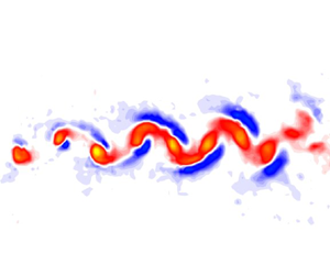
The normalized spanwise (i.e. axial) flow fields,  $w^*= \langle w\rangle /V_{swm,i}$, are shown on figures 8(b,d, f,h) and 9(b,d, f,h). In these figures the red/yellow coloured contours indicate positive spanwise flow away from the wall, while the blue/cyan contours indicate negative spanwise flow toward the wall. The positive axial flow first appeared at $z=r_{c,i}$ and then progressively at the farther data planes for both cases, as expected. The axial flow expanded away from the wall faster for the high $\varGamma$ case due to the higher axial flow speeds, e.g. in the low $\varGamma$ case in figure 8, the first positive axial flow region at $x\approx 5r_{c,i}$ appears only at the $z=r_{c,i}$ plane, whereas in the case of high $\varGamma$ in figure 9 the same appears at both $z=r_{c,i}$ and $2r_{c,i}$ planes. For both the low and high $\varGamma$ cases, the positive spanwise flow was initially found to be spatially coincident with the vortex core of either sign with peak magnitudes of the order of the maximum swirl speed, consistent with previous results of Bohl & Koochesfahani (Reference Bohl and Koochesfahani2004). Interestingly, the negative spanwise flow toward the wall was also clear in the two near-wall planes, where they were always located on the outer (free-stream) edges of the vortices, with magnitudes that were lower (nominally 0.5 $V_{swm,i}$) than the primary positive axial flow.
The structure of the spanwise flow fields of both cases were consistent with the vorticity fields previously discussed. Consider first the near-wall measurement planes ( $z=r_{c,i}$ and $2r_{c,i}$). For the low $\varGamma$ case, the regions of spanwise flow stretched into oblong structures qualitatively similar in shape, and spatially coincident, to the vorticity structures at the same downstream distance. The axial flow, like the vortical structures, remained isolated and distinct throughout the measurement domain. However, the structure of the spanwise flow for the high $\varGamma$ case changed from isolated regions to a more continuous sheet-like region farther downstream in the regions where primary vortices had broken up into multiple smaller compact regions of vorticity. Distinct maxima in the axial flow were, however, observed and found to be spatially coincident with the locations of the vortical structures. The axial flow field at these planes showed a marked decrease in intensity at the downstream edge of the measurement planes consistent with the disappearance of the vortical structures for these measurement planes.
The spanwise flow fields for  $z=10r_{c,i}$ and $20r_{c,i}$ were qualitatively different from the near-wall cases. For the low $\varGamma$ case, axial core flow was observed in isolated regions spatially coincident with the location of the vortex cores. No reverse spanwise flow was observed at these planes for this case. Given the relatively weak positive spanwise core flow at this measurement plane, it was likely that any negative axial flow was at a level below the measurement uncertainty of the current experiments. As expected, the high $\varGamma$ case showed notably earlier measurable axial flow when compared with the low $\varGamma$ case. The axial flow developed into the sheet-like structure of the near-wall measurement planes with measurable negative spanwise flow only near the downstream edge of the measurement domain at the $z=10r_{c,i}$ plane. Previous line tagging measurements of Bohl & Koochesfahani (Reference Bohl and Koochesfahani2004) had also observed the continuous sheet-like structure of axial flow just mentioned. At $z=20r_{c,i}$ the spanwise flow entered the flow field as single peaked, isolated structures, but changed to multi-lobed or hollow profiles for $x>30r_{c,i}$, see figure 9. This may be a result of the influence of the opposite sign axial flow in the vortices cut by the far cutting wall and the proximity to the midspan of this measurement plane where one would expect the axial flow from the far wall to meet to enforce the zero velocity boundary condition. The low $\varGamma$ case did not show the same reduction in the spanwise flow at this plane. This likely would have been observed if the measurement region were longer downstream as the weaker axial flow only begins to enter the flow field at the end of the measurement domain for the low $\varGamma$ case.
3.3. Mean vorticity and spanwise velocity fields after interaction
The unique characteristics of the instantaneous spanwise vorticity and axial flow fields just discussed for different spanwise planes lead to interesting consequences for their mean fields. Mean normalized vorticity fields are shown in figures 10(a,c,e,g) and 11(a,c,e,g) for the low and high  $\varGamma$ cases, respectively. It is noted that the maximum contour levels are set below the maxima for both the vorticity and spanwise flow in these figures so that the details of the lower mean levels can be more clearly observed. In the low $\varGamma$ case, figure 10, the primary regions of mean vorticity were located symmetrically about the $y$-axis of the flow field. The mean vorticity fields confirmed that the region of primary vorticity spread vertically during the initial interaction and then remained nominally equally spaced for the near-wall planes. Closest to the wall ( $z = r_{c,i}$), the regions of secondary vorticity that resulted from the breakup of the initially compact regions of vorticity led to a mean secondary vorticity field that appeared mostly outside of the regions of the primary vorticity, except for the far downstream portion of the measurement domain. The mean vorticity fields for the $z=10r_{c,i}$, $20r_{c,i}$ far-field planes did not show significant vertical widening in the streamwise direction that was observed at the near-wall planes. Instead, they were characterized by two well-defined peaks of opposite vorticity with their transverse location and sign consistent with the isolated vortex array of the traditional Kármán street (see figure 8), with only a slight widening of the array in going from $z=10r_{c,i}$ to $20r_{c,i}$. Interestingly, these characteristics persisted for the primary mean vorticity in the two near-wall planes as well, in spite of the near-wall interactions and appearance of secondary vorticity regions.

Figure 10. (a,c,e,g) Normalized mean vorticity,  $\omega ^*$ , and (b,d, f,h) spanwise velocity, $w^*$ fields at multiple span locations for the low $\varGamma$ case.

Figure 11. (a,c,e,g) Normalized mean vorticity,  $\omega ^*$ , and (b,d, f,h) spanwise velocity, $w^*$ fields at multiple span locations for the high $\varGamma$ case.
The normalized mean vorticity fields for the high  $\varGamma$ case, figure 11, exhibited a fundamentally different behaviour compared with the low $\varGamma$ case just discussed, as a consequence of the different vorticity dynamics previously described in connection with figure 9. In the plane closest to the wall ( $z=r_{c,i}$), the mean vorticity was initially characterized by two well-defined peaks of opposite vorticity whose transverse location and sign were consistent with the isolated vortex array of the reverse Kármán street depicted in figure 9. By $x\approx 15r_{c,i}$, the breakup of each primary vortex of either sign into two (a larger primary and a smaller secondary) vortices of the same sign resulted in the bifurcation of each mean vorticity peak into two, with the weaker thinner branch forming on the outside of the primary branch. Meanwhile, after breakup the primary vortices of either sign changed their transverse orientation and became aligned with each other nearly perfectly along a straight line, resulting in zero mean vorticity of the primary branch in the region in the range $x\approx 24-30r_{c,i}$ . Beyond this region the primary non-zero mean vorticity reappeared, but with its transverse orientation switched, a consequence of the change in the vertical orientation of the primary vortices described earlier in the phase-averaged vorticity map of figure 9.
The flow field characteristics described above at the plane closest to the wall ( $z = r_{c,i}$) also occurred at $z=2r_{c,i}$, but the locations of the mean vorticity peak bifurcation and reappearance of mean vorticity peaks with switched orientation moved slightly downstream. The first far-field plane ( $z = 10 r_{c,i}$) showed evidence of the same features near the downstream edge of the measurement plane, but the plane farthest away from the wall ( $z = 20 r_{c,i}$) did not reveal those features over the measurement domain and the mean vorticity field was, instead, characterized throughout by two well-defined peaks of opposite vorticity corresponding to the isolated vortex array of the reverse Kármán street (see figure 9).
The normalized mean spanwise flow fields, shown in figures 10(b,d, f,h) and 11(b,d, f,h) for the low and high  $\varGamma$ cases, reveal a common set of features regardless of the differences in the underlying vortical structure and interactions. Whereas the mean vorticity fields showed zero mean vorticity in the centre of the vortex array due to the alternating sign of vortices, the mean spanwise velocity showed generally positive axial flow away from the wall in the centre of vortex arrays due to the positive axial flow in the vortex cores for either sign vortices. The magnitude of the mean positive spanwise flow in the vortex array centre is determined by the strength of the axial flow in the vortex core, the core size, and the transverse separation between alternating sign vortices. The low $\varGamma$ case at $z=r_{c,i}$ (figure 10), and the early portion of the high $\varGamma$ case at $z=r_{c,i}$ (figure 11), are examples of situations where the mentioned parameters led to low levels of positive axial flow in the centre (near zero in some areas), and the maximum was found in two distinct regions that were spatially coincident with the locations of the peak vorticity. On the other hand, the downstream evolution of maximum axial flow in the centre for the high $\varGamma$ case at $z = r_{c,i}$ , 2 $r_{c,i}$, and 10 $r_{c,i}$ (figure 11) showed the regions of the maximum mean axial flow were located at the same downstream region where the primary alternating sign vortices changed their transverse orientation and became nearly perfectly aligned with each other. Note that negative mean spanwise flow was found outside of the region of mean positive spanwise flow, which was consistent with the location of the negative flow shown in the phase-averaged results.
The phase-averaged and mean fields, discussed in §§ 3.2 and 3.3, provide information about the instantaneous structure and average characteristics of the vorticity and spanwise velocity distributions. In the next section we discuss the dynamic characteristics of the flow in term of the evolution of selected vortex properties.
3.4. Vortex parameters
The phase-averaged vorticity and spanwise velocity data, such as those in figure 9, allow us to interrogate the downstream evolution of select vortex parameters, presented in figure 12 for the high  $\varGamma$ case. The dynamics that is discussed was more pronounced for this case, but the qualitative description was similar for the low $\varGamma$ case. The parameters considered are the core radius, peak vorticity and peak spanwise velocity. Their values were found by identifying a vortex as it entered the measurement region and tracking its location and properties at each phase as it convected downstream. In this way the characteristics of the vorticity and spanwise flow fields were quantified throughout the entire measurement domain. Both the positive and negative vortices were tracked and the measured values were consistent for both. Peak vorticity values are shown for streamwise locations were the vortices remained as well-defined structures with a clear primary core, as the interpretation of the ‘peak vorticity’ was less clear after the vortices became distorted or broke up. The peak vorticity and vortex core data in figure 12 also include baseline results at the centre-span location without the cutting walls present from Bohl & Koochesfahani (Reference Bohl and Koochesfahani2009) for reference. Note that these two vortex parameters, which for the current data are from the flow that was strongly three-dimensional, agreed well initially with the properties from the centre-span data.

Figure 12. Vortex parameters ( $r_c^*$, $w_p^*$, $\omega _ p^*$) at multiple span locations for the high $\varGamma$ case. Baseline data are from centre span without the cutting walls (Bohl & Koochesfahani Reference Bohl and Koochesfahani2009).
The vortex core radius,  $r_c^*$, initially followed the expansion trend of the baseline case, with the near-wall planes showing rapid increases in the vortex radius as the vortices distorted and the axial flow was generated. This was also observed for the far-field planes, however, the increased rate of expansion was delayed to progressively farther downstream locations. The initiation of the rapid expansion of the core was spatially coincident to the spatial location where the axial flow was first measured for all measurement planes. This indicated that the rapid expansion of the vortex radius was, at least initially, associated with the development of the axial flow. Smaller scale local oscillations in the core radius, which will be discussed in subsequent discussion, were also observed.
The peak spanwise velocity,  $w_p^*$, showed slow developing (i.e. long spatial wavelength) trends along with a more local (i.e. short spatial wavelength) dynamics. Consider first the global trends in the data. All measurement planes showed initiation of axial flow that increased to a peak level and then decreased. The downstream location at which the axial flow was initiated at each plane progressively increased with spanwise plane location, as expected given the spanwise flow was generated at and then convected away from the wall. The global maximum values decreased with increasing distance away from the wall. The location of the overall maximum value for each spanwise plane moved downstream as the distance from the wall increased with the exception of the $z=20r_{c,i}$ plane. Here, the global maxima occurred earlier than was observed for the $z=10r_{c,i}$ plane. This was most likely due to the $z=20r_{c,i}$ measurement plane being near the centre of the span where spanwise flow from the opposite wall will have some influence and likely inhibited a higher magnitude of axial flow from being developed.
Within these overall trends smaller, local maxima/minima were also observed in the profiles. Figure 13 shows  $w_p^\ast$ for $z=10 r_{c,i}$ and 20 $r_{c,i}$ on the same plot for comparative purposes. Several local maxima/minima were observed at both spanwise planes. The first local maxima (S1) at each measurement plane were labelled with solid lines and the second (S2) by dashed. Other local minima were observed but not labelled on the plot for clarity. These data indicated the local maxima/minima, i.e. ‘spikes’, were not isolated incidents, but disturbances that convected away from the wall through multiple measurement planes. Further, these local spikes, even in the near-wall region could not be solely due to the initial cutting of the vortices as they continue to form well after the vortex was cut and the axial flow is initiated. These effects will be discussed in detail in §§ 3.5 and 3.6.

Figure 13. Peak axial flow,  $w_p^*$, as a function of downstream distance for the high $\varGamma$ case.
The peak vorticity, figure 12, showed a rapid decline in magnitude and interestingly also local oscillations, or spikes, for the near-wall planes. These effects were also observed at the far-field planes, although they were again delayed depending on the spanwise location of the plane. There are two possible explanations for this phenomenon. First, re-organization of the vorticity and circulation created dynamic changes in the peak vorticity levels. Second, local variations in the vortex radius (i.e. a vortex stretching effect) changed the vorticity levels. The evolution of the vorticity in the near-wall planes was complicated by both the initiation of the axial flow and distortion of the vortex due to the proximity of the wall. In the far-field region the vorticity remained in isolated structures and the re-organization of the vorticity was a less likely explanation. Therefore, vortex stretching was more likely the source of these local oscillations, at least in the far field.
Bohl & Koochesfahani (Reference Bohl and Koochesfahani2009) investigated the downstream evolution of the peak vorticity for the 2-D baseline case also presented in this work. They showed that the rate of decrease in the peak vorticity level showed a distinct change as the vortex convected downstream. The initial decrease in the peak vorticity was found to be due to diffusion of the vortex core. The rate of decrease in the peak vorticity then showed a distinct change and became faster than if diffusion alone were considered. They were able to show that the presence of even a small velocity gradient in the spanwise direction axial flow ( ${\partial w}/{\partial z}$) within the vortex core caused the additional decrease in the peak vorticity. In that work velocity gradients of the order of ${\partial w}/{\partial z}=0.1\,{\rm s}^{-1}$ compared with dimensional vorticity values 2–3 orders of magnitude larger were sufficient to produce the observed changes. The trends for the peak vorticity for the $z=10r_{c,i}$ and $20r_{c,i}$ planes of the current data were consistent with this model. Of note is that the current data, which measured vorticity and axial flow simultaneously, showed that the location where the rate of decrease changed was upstream of the point at which the axial flow itself was observable, supporting the conclusion that very small spanwise velocity gradients have a significant effect on the vortex dynamics.
3.5. Axial flow development
Axial flow data discussed so far were at only 4 selected spanwise locations and their purpose was to investigate in detail the spatial development in the streamwise,  $x$, direction. Now we focus on the spanwise development of axial flow with finer resolution in $z$, but at specific downstream, $x$, locations. Line tagging MTV was applied here as it allowed finer spatial resolution in the spanwise direction ( $z$) and a more detailed mapping of the axial flow than the sMTV experiments. Measurements were taken at multiple (16) span locations from 0.6 $r_{c,i} \le z \le 25 r_{c,i}$ with an approximate spacing of $1.6r_{c,i}$ and from $2.5r_{c,i} \le x \le 67.5 r_{c,i}$ with steps of $2.5r_{c,i}$. Contour maps of the maximum positive and negative spanwise flows over the entire spatial extent for the two cases being discussed are shown in figure 14. Both cases show that the positive spanwise core flow began near the wall and moved towards the centre of the tunnel with increasing downstream distance, as expected. The axial flow ‘front’ (i.e. the boundary between the spanwise flow/no spanwise flow) advanced more rapidly for the higher circulation case. Both cases showed nominally the same normalized axial flow levels with the highest levels measured of the order of $V_{swm,i}$, indicating that the spanwise flow scaled with the swirl speed, and by extension, strength of the vortex. The region where the axial flow was nominally equivalent to the swirl speed was confined to the region near the wall for the low $\varGamma$ case. The high $\varGamma$ case showed that the region of high positive spanwise flow moved away from the wall with increasing downstream distance with a pronounced region of low spanwise flow near the wall. These data were qualitatively and quantitatively consistent with the sMTV results which showed the loss of the vortical regions and spanwise flow near the wall. Variation in the axial flow speed was observed along the axial flow front for both cases, although it was much more pronounced for the high circulation case.

Figure 14. Contour plot of peak positive (a,c) and negative (b,d) normalized axial flow,  $w _p^*$, over the measurement domain.
The peak negative spanwise flow fields were found to be aligned with regions of the highest axial flow, near the cutting walls for the low  $\varGamma$ case and initially along the wall then angling into the flow field for the low $\varGamma$ case. The magnitude of the peak negative spanwise flow was higher for the low $\varGamma$ case than for the high $\varGamma$ case. This is again consistent with the phase-averaged spanwise flow fields in figure 8 and 9 where the negative spanwise flow was limited to isolated structures.
The peak positive spanwise flow data in figure 14 were used to plot spanwise profiles along the axial flow front ( $2.5< x/r_{c,i}<10$) for the high $\varGamma$ case to investigate the initial dynamics of the positive axial flow within the vortex cores, figure 15. It is again important to recall that these data are from phase-averaged results that were taken at multiple locations and therefore the features they display are repeatable in both time and space. These profiles show that as the axial flow front propagated away from the wall a clear local overshoot or ‘spike’ in the axial flow velocity was observed. These initial local overshoots are identified in figure 15 by the solid arrows for each downstream location. The velocity spike followed the front boundary as it progressed away from the cutting wall. Spikes at the axial flow front boundary were observed for all circulation cases studied, although the magnitude of the spike was progressively weaker for lower $\varGamma$ cases. The profile at $x=10r_{c,i}$ also showed evidence of other velocity spikes behind the axial flow front indicating that these features continued to be formed as the vortex interacted with the cutting walls and were not limited to the initial cutting of the vortex.

Figure 15. Spanwise profiles of peak axial flow vs downstream distance for the high  $\varGamma$ case.
The results thus far show that the initiation and development of the axial flow within the vortex cores had significant effects on the vorticity distribution and core size of the vortex array. These results were suggestive that disturbances were generated near the wall and propagated away from the wall along the vortex. This dynamics is explored and compared with the analytic area-varying wave model of Lundgren & Ashurst (Reference Lundgren and Ashurst1989) in the following section.
3.6. Area-varying waves
Lundgren & Ashurst (Reference Lundgren and Ashurst1989) examined the development and propagation of area-varying waves on vortices using an analytic model. The current data allow examination of the propagation along the vortex core of the disturbance caused by the impulsive vortex cutting by a thin plate, and its connection to travelling area-varying waves predicted by Lundgren & Ashurst (Reference Lundgren and Ashurst1989). We focus on the first disturbance launched during the initial cutting of the vortex, where the vortex retains its Gaussian nature in the areas interrogated and its characteristics can be quantified without much complication. Lundgren & Ashurst (Reference Lundgren and Ashurst1989) used the gas dynamics equations as an analogous description of the behaviour of area-varying waves on a vortex tube. They defined an equivalent ‘speed of sound’ in their equation (4.7) as
 \begin{equation} c^2=\frac{\varGamma ^2}{8{\rm \pi} A}. \end{equation}
Here,  $\varGamma$ is the circulation of the vortex and $A = {\rm \pi}r_c^2$ is it's area. The authors considered a sharp edged vortex with uniform vorticity within the core (i.e. ‘flat top vortex’), where the maximum swirl speed, $V_{swm}$, is defined by
 \begin{equation} V_{swm}=\frac{\varGamma}{2{\rm \pi} r_c}. \end{equation}
When (3.2) and (3.3) are combined, the non-dimensional ‘sound speed’, normalized by the maximum swirl speed, for a flat top vortex model simplifies to
 \begin{equation} \frac{c}{V_{swm}}=V^*_{FT}=\frac{1}{\sqrt{2}}=0.707. \end{equation}
The vortices in this work are well described by a Gaussian vortex model, as previously discussed. The maximum swirl speed for this vortex model using (3.1) is found when  $r/r_c=1.12$. Using the maximum swirl speed of a Gaussian vortex for normalization in combination with (3.2) leads to the non-dimensional wave speed for the Gaussian vortex model being given by
 \begin{equation} \frac{c}{V_{swm}}=V^*_{G}=\frac{1}{\sqrt{2}}\frac{1}{0.6382}=1.11. \end{equation}
 The data in figures 13 and 15 show evidence of disturbances that propagate along the vortex core. Two estimates of the propagation speed of this disturbance speed were calculated using the line tagging data, which were available for the entire circulation range studied, for comparison with the analytic model. The spatial location of the axial flow ‘front’ was defined by the span location where  $\langle w\rangle _{peak} = 0.5$ cm s $^{-1}$. This level, while arbitrary, was chosen to be slightly above the uncertainty level in the measurements allowing for the determination of the location of the initial axial flow front to be made. We note that this choice of threshold level did not significantly affect the results that follow. Figure 15 shows the front threshold as the vertical dashed line and the spanwise, $z$, location of this position is indicated by the green arrows in that figure. The convection time was calculated using the pre-interaction convection speed, $U_{c,i}$, multiplied by the streamwise distance between measurement locations. The front speed, $V_f$, was determined by differentiation of a linear least squares fit of the spanwise location of the front with time. The intent of the calculation of the front speed with this definition was to compare the propagation of the leading edge of the axial flow with the propagation speed of first disturbance observed on the vortex cores. The propagation speed of the first disturbance, $V_d$, was determined in a similar way. However, in this case the spanwise location of the first local velocity maximum, shown with the solid arrows in figure 15, was used to define the spanwise location of the first disturbance. Data were again fit using a linear least squares curve and differentiated to determine the disturbance speed, $V_d$.
The stereoscopic data provided an independent method for calculating the propagation speed of the initial disturbance,  $V_{ds}$, for the low and high $\varGamma$ cases. The tracking data for the peak spanwise flow, shown in figures 12 and 13 for the high $\varGamma$ case, were replotted as a function of time instead of space. We note that for these data time was known directly instead of via calculation using the initial convection speed. The time of the occurrence of the first spanwise flow spike was determined for each of the measurement planes, which defined the spanwise location. These data were also fitted using a linear least squares and then differentiated with respect to time. All disturbance speeds were then normalized using the maximum pre-interaction swirl speed, $V_{swm,i}$, which was taken as analogous to the maximum swirl speed, $V_{swm}$, for the analytic model.
The results of the preceding analysis are plotted in figure 16. The dimensional speeds, figure 16(a), showed a linear increase with vortex circulation as well as good agreement between the line tagging and stereoscopic data. The normalized speeds are shown in figure 16(b). The dashed line is the theoretical normalized sound speed for the Gaussian vortex model from (3.5). The solid line is the theoretical normalized sound speed for the flat top vortex model from (3.4) and is provided for reference. Experimental results are shown with symbols. The results shows that the normalized disturbance speeds,  $V^*_f$ and $V^*_d$, were nominally constant and agreed well with the results from the stereoscopic data, $V^*_{ds}$. More significantly, these results indicated that the propagation speed of the first disturbance matched the analytic sound speed proposed by Lundgren & Ashurst (Reference Lundgren and Ashurst1989).

Figure 16. (a) Dimensional and (b) normalized axial flow disturbance speeds. Here, VG  ${*}$: analytic equivalent sound speed for a Gaussian vortex; ${V^*}_{FT}$: analytic equivalent sound speed for a flat top vortex from Lundgren & Ashurst (Reference Lundgren and Ashurst1989).
Lundgren & Ashurst (Reference Lundgren and Ashurst1989) showed in their equation (4.14) that the speed at which disturbances propagate along the vortex core depends on the equivalent sound speed, the area ratio up and down stream of the disturbance and the speed of the axial flow into which the disturbance is propagating. For cases with small variations in the area of the vortex core and no axial flow ahead of the disturbance, the wave speed of a disturbance simplifies to the equivalent sound speed,  $c$. These conditions will be shown to be met for the initial disturbance caused by the initiation of the axial flow. The data in figure 16 were, therefore, suggestive that small amplitude area-varying waves were generated on the vortex cores as the axial flow was first initiated and then propagated through the vortex cores.
Figure 17 shows  $r_c^*$, $w^*$ and $\omega ^*$ plotted on the same figure at $z=10r_{c,i}$ and $20r_{c,i}$ for the high $\varGamma$ case. These span locations were chosen for analysis because the vortices remained relatively undistorted and well defined over the measurement domain. Note that the vertical axis of the curves are offset to allow the curves to be displayed on the same figure without significant overlap. The intent of these plots is to show spatial coincidence of the features in each profile, not relative scales of the plotted values. Changes in the vortex core radius were difficult to distinguish in figure 17 because of the naturally increasing core radius as the vortex convected downstream and because these changes were small. The variable $\Delta r^*$ was calculated to highlight the local changes in the vortex core radius in the following way. The core radius was first smoothed using a $\pm$30 point moving spatial average. This value was subtracted from the local vortex core radius and divided by $r_{c,i}$ to provide a local normalized difference, $\Delta r^*$ at each streamwise location.

Figure 17. Correlation of spatial features of vortex parameters for the high  $\varGamma$ case.
At  $z=10r_{c,i}$ a series of local maxima and minima were observed in the peak vorticity as a function of the downstream distance. The first local minimum in the peak vorticity (solid line) corresponded to a small but measurable increase in $r_c^*$, seen as a local maximum in $\Delta r^*$. There was also an associated local maximum in $w^*$. This was followed by a local maxima (dashed line) in the peak vorticity which was correlated to a minimum in the core radius ( $\Delta r^*$) and axial flow. The vortex core radius showed the least pronounced local maximums and minimums. For example, the variation in $r_c^*$ for the first local peak was relatively small, at approximately $\Delta r^*\approx 1.3\,\%$. This level was significant, but near to the noise level in the radius estimation. The subsequent vorticity peaks were less intense, and the corresponding area changes were also smaller. At $z=20r_{c,i}$ the correlation between the vorticity and spanwise velocity was clear for the first three vorticity spikes. Changes in the vortex core radius were again small ( $\Delta r^*<1\,\%$) but visible at this span location. These trends were also observable for the low $\varGamma$ case (not shown here). However, for this case the weaker initial vortex along with the distortion/reorganization of the vorticity and made this correlation less clear.
These results reveal important aspects of the dynamics of the development and progression of the axial flow within the vortex. The axial flow developed and then strengthened as it progressed away from the cutting walls. This led to a surge in the axial flow that created an increase in the vortex area which in turn resulted in a local decrease in the peak vorticity. The vortex radius decreased and the peak vorticity increased after the disturbance on the vortex core propagated past the spanwise measurement location. This view is of course simplistic as other dynamics (e.g. diffusion/expansion of the vortex) are occurring simultaneously, creating more complicated flow dynamics.
The data do, however, support the existence of travelling small amplitude, area-varying waves on the vortex core. Recall that the analytic wave speed simplified to the analytic sound speed,  $c$, assuming small area variation and an initial axial flow velocity of $w=0$. These simplifications were met for the first disturbance on the vortex cores where the variation in the vortex core area was small ( ${<}1.3\,\%$) and there was no axial flow ahead of the disturbance. The measured disturbance speeds shown in figure 16 were shown to be nominally equal to the associated sound speed, confirming the analytic model proposed by Lundgren & Ashurst (Reference Lundgren and Ashurst1989). Moreover, the characteristics of the peak vorticity and axial flow, which are more pronounced and easier to measure than the vortex core area for small disturbances, appear to also be indicators of the existence and spatial/temporal locations of area-varying waves.
4. Conclusions
The structure of 2-D line vortices cut impulsively by a thin plate, and the induced axial flow, were quantified using line tagging and stereoscopic MTV for vortices of varying strength. Two vortices with circulation levels  $\varGamma _i=21$ to $\varGamma _i=55\,{\rm cm}^{2}\,{\rm s}^{-1}$ were investigated in detail. These data revealed many dynamics of the vortex interaction with the cutting walls. In the near-field region, the vortices distorted and reorganized into multiple regions of vorticity near the wall, with the profile becoming non-Gaussian and asymmetric. The vortices were found to develop hollow vorticity profiles for several conditions, although the evolution from Gaussian to hollow was not a result of decreasing peak vorticity, but instead distortion and re-distribution of the vorticity. In the far field, the vortices remained Gaussian like with a decreasing peak level as the convect downstream. The current data confirmed the inference of Bohl & Koochesfahani (Reference Bohl and Koochesfahani2009) that the combined effects of diffusion and axial flow gradients were responsible for the rapid reduction in the peak vorticity level.
Spanwise, i.e. axial, flow in the core of the vortices was measured. The maximum axial flow speed was found to be significant and varied between 60 % and 100 % of the maximum swirl speed of the vortices for the circulation levels investigated. The axial flow was initially located within the vortex cores. A weaker reverse spanwise flow was also observed outside of the vortex cores. The distribution of the spanwise flow within the vortex core was qualitatively different depending upon the span location and varied from Gaussian like, to multi-lobed, to sheet like. The transition of the axial flow structure from isolated to sheet like was observed in the data for the high circulation case. This change in structure occurred over the same region as the break-up of the vortices was observed.
Local maxima and minima in the spanwise flow and peak vorticity were observed to form near the cutting walls. These disturbances moved away from the cutting walls as the vortices convected downstream. The spatial and temporal locations of these ‘spikes’ were correlated between each other and also to local changes in the core radius. The change in core radius was small (less than 1.3 %) and most apparent for the highest circulation case.
Analysis of the data showed that small amplitude area-varying waves developed on the vortex cores near the cutting wall soon after the axial flow was initiated. The expansion and contraction of the vortex core size was consistent with the observed changes in the peak vorticity and axial flow speed. Specifically, as the axial flow speed increased the vortex radius expanded locally and the peak vorticity decreased, as expected. This was followed by a decrease in the axial flow speed, a decrease in the vortex core radius and an increase in the peak vorticity. The cycle appeared to repeat after the axial flow was established as disturbances continued to be generated at the wall and convect along the vortex core. These results indicate that the local maxima and minima in the peak vorticity and axial flow were markers for the passage of an area-varying wave on the vortex core.
The disturbance speed of the initial area-varying wave was compared with the analytic model of Lundgren & Ashurst (Reference Lundgren and Ashurst1989) for a Gaussian vortex. The propagation speed of the first disturbance agreed with predictions from the analytic model. The current data therefore provide experimental confirmation of both the existence of area-varying waves on a vortex and the applicability of the analytic work of Lundgren & Ashurst (Reference Lundgren and Ashurst1989) to predict the behaviour of these waves.
The current data reveal that the initial interaction of a vortex array cut by a solid boundary, and the subsequent vortex dynamics, are rich in physics. The dynamics near the wall is not fully understood from the current study due to the relatively large spatial distance between the measurement planes, and the closest near-wall plane being outside the undisturbed boundary layer of the cutting wall over the initial vortex–wall interaction region. The data presented here indicate that, after the first disturbance launched along the vortex core due to the initial interaction of vortex and cutting plate, additional disturbances are generated near the wall that also propagate along the vortex cores. These disturbances are likely to be different in their generation physics due to the distortion of the vortex cores near the wall and interaction with the developing boundary layer on the wall. Volumetric boundary layer resolved measurements are needed to fully reveal the detailed physics of the initial formation of the axial flow in the vortex core near the wall as well as the subsequent vortex dynamics and boundary layer development. Such measurements would also extend the current understanding of flow physics of single vortex interaction with a wall to vortex array interaction with a wall.
Funding
This work was supported by the MRSEC Program of the National Science Foundation, Award Numbers DMR-9400417, and DMR-9809688.
Declaration of interests
The authors report no conflict of interest.


