


Introduction
Icebergs are a major means for moving fresh water from the Antarctic Ice Sheet (AIS) to the Southern Ocean, with icebergs contributing an estimated ~50% of this transfer (Depoorter et al. Reference Depoorter, Bamber, Griggs, Lenaerts, Ligtenberg, van den Broeke and Moholdt2013). In contrast to the Northern Hemisphere polar oceans, where icebergs tend to be at most a few hundred metres in length (Dowdeswell et al. Reference Dowdeswell, Whittington and Hodgkins1992), the majority of this ice-mass loss from the AIS occurs in the form of episodic calving of very large to giant icebergs (Silva et al. Reference Silva, Bigg and Nicholls2006). These can be tens to hundreds of kilometres in size when they break off from ice shelves bordering the AIS; the largest observed since the beginning of the satellite era was iceberg B15, which measured 295 × 37 km when it calved from the Ross Ice Shelf at the end of March 2000 (https://www.nsf.gov/od/lpa/news/press/00/pr0012.htm). Such large icebergs, and their often-substantial fragments, can survive for years to decades because of their size, especially as most remain within the westward-flowing Coastal Current around Antarctica until they reach the Weddell Sea gyre and are expelled into the Antarctic Circumpolar Current (ACC) of the South Atlantic (Bigg Reference Bigg2016), almost irrespective of where they calve from the main AIS. This longevity means that their meltwater, released sedimentary and biological debris carried by the ice and entrainment of sub-surface nutrients and seawater within meltwater plumes (Smith et al. Reference Smith, Sherman, Shaw and Sprintall2013) can influence the ocean over a spatially large and temporally long scale.
The position and approximate size of ‘giant’ icebergs (defined to be > 18 km in length) have been monitored routinely for navigational reasons using remote sensing since the 1970s (Budge & Long Reference Budge and Long2017), and a spatial and chronological naming convention exists for these giant icebergs (Bigg et al. Reference Bigg, Marsh, Wilton and Ivchenko2014). However, despite their potentially large and movable impact on the ocean's physics, chemistry, biology and sedimentation, the difficulty of carrying out either field or remote sensing studies in a sustained manner has limited the number of extant studies of giant icebergs. Some studies have examined the physical impacts of such icebergs within the coastal sea-ice environment. These have involved mostly remote monitoring of large iceberg collisions through hydroacoustic or seismic signals (e.g. Chapp et al. Reference Chapp, Bohnenstiehl and Tolstoy2005, Talandier et al. Reference Talandier, Hyvernaud, Reymond and Okal2006, MacAyeal et al. Reference MacAyeal, Okal and Aster2008, Martin et al. Reference Martin, Drucker, Aster, Davey, Okal, Scambos and MacAyeal2010), melting during long-term grounding (Gordon et al. Reference Gordon, OrsI, Muench, Huber, Zambianchi and Visbeck2009) or movement within concentrated pack ice (Wesche & Dierking Reference Wesche and Dierking2015, Han et al. Reference Han, Lee, Kim and Kim2019). Others have considered specific benthic or faunal responses of the coastal Antarctic ecosystem to the disruption accompanying the calving and passage of giant icebergs (e.g. Whitehead et al. Reference Whitehead, Lyver, Ballard, Barton, Karl and Dugger2015, Wilson et al. Reference Wilson, Turney, Fogwil and Blair2016, Barnes et al. Reference Barnes, Fleming, Sands, Quartino and Deregibus2018). However, the three main field studies of giant icebergs were carried out in the Weddell Sea (for summaries, see Smith et al. Reference Smith, Robison, Helly, Kaufmann, Ruhi and Shaw2007, Smith Reference Smith2011) over a few weeks each time. They showed that these giant icebergs had significant impacts on their nearby physical (e.g. Helly et al. Reference Helly, Kaufmann, Stephenson and Vernet2011), biological (e.g. Vernet et al. Reference Vernet, Smith, Cefarelli, Helly, Kaufmann and Lin2012) and chemical (e.g. Shaw et al. Reference Shaw, Raiswell, Hexel, Vu, Moore, Dudgeon and Smith2011) environment, even extending to an impact on carbon sequestration (Smith et al. Reference Smith, Sherman, Shaw, Murray, Vernet and Cefarelli2011). This significant but local impact on biological productivity was also found in a glider study of a large iceberg in the same region more recently (Biddle et al. Reference Biddle, Kaiser, Heywood, Thompson and Jenkins2015). The visible satellite image analysis by Duprat et al. (Reference Duprat, Bigg and Wilton2016) extended the temporal and physical scope of this work through examining the open ocean paths of 17 giant icebergs over a decade, following their impacts on ocean biology through a total of 175 images covering areas pre- and post-iceberg passage. They found a mean several-fold increase in chlorophyll levels well away from the icebergs, with a discernible impact at times stretching hundreds of kilometres up- or downstream of the giant iceberg. These results were confirmed by a more systematic remote sensing study by Wu & Hou (Reference Wu and Hou2017) covering icebergs of all sizes over a 20 year period.
Nevertheless, following individual large icebergs through substantial periods of their lifetime, and so understanding the evolution of their physical and biological impacts on the surrounding ocean, remains rare. The concentration of those studies that do exist is on the meltwater input into the ocean and the variation in its rate of input over time. Thus, Jansen et al. (Reference Jansen, Schodlok and Rack2007) followed the melting history of the giant iceberg A38b over the 6 years from its calving at the Ronne Ice Shelf of the Weddell Sea in 1998 to its grounding prior to break-up off South Georgia in 2004 using a range of radar, altimetric and visible image remote sensing instruments. They found that the weakest melting rates occurred during the passage of A38b through the open water of the Scotia Sea, whilst the strong tidal currents within the ice pack of the Weddell Sea and the frictional impact of grounding off South Georgia both enhanced melting rates significantly. In a more local but similarly long-lived study, Robinson & Williams (Reference Robinson and Williams2012), using in situ data, found that the two massive giant icebergs B-15 and C-19 perturbed the ocean salinity, and so regional oceanography, in McMurdo Sound for some time whilst the icebergs remained within the area. The meltwater from these icebergs cooled and freshened the upper water column, reducing the surface circulation and, in the case of C-19, eliminating the Ross Sea polynya for several years. This freshening also shifted the core location of deep-water formation in the south-western Ross Sea. A comparison of the changes in two icebergs, C28a and C28b, associated with the break-up of the original C28 giant iceberg, showed that there were differential changes in freeboard and area even whilst the two product icebergs were in the same vicinity off the Mertz Ice Tongue of East Antarctica (Li et al. Reference Li, Shokr, Liu, Cheng, Li, Wang and Hui2018).
Two of the most ambitious studies examined melting whilst giant icebergs were in the open ocean and so away from the complicating influence of sea ice (Bouhier et al. Reference Bouhier, Tournadre, Rémy and Gourves-Cousin2018, Braackmann-Folgmann et al. Reference Braackmann-Folgmann, Shepherd, Gerrish, Izzard and Ridout2022). Bouhier et al. (Reference Bouhier, Tournadre, Rémy and Gourves-Cousin2018) examined icebergs B17a (during its passage across the South Atlantic) and C19a (in the Pacific Ocean), finding that thermodynamic rather than fluid dynamics-based melting formulations worked better in predicting iceberg melting. They were also able to construct a bulk model of fragmentation depending on ocean temperature and iceberg velocity, as they followed the two icebergs long enough to detect the final fragmentation process, when melting accelerates. Braackmann-Folgmann et al. (Reference Braackmann-Folgmann, Shepherd, Gerrish, Izzard and Ridout2022) used detailed remote sensing tracking of iceberg A68a from its calving from the Larsen C Ice Shelf in November 2017 until its break-up near South Georgia in late 2020 to estimate a basal melt rate in the open South Atlantic of up to ~7 m/month.
In the current work, these previous studies are extended by considering the impact of varying iceberg size on an iceberg's meltwater impact on the ocean's properties and on its biological production. A cluster of three large icebergs that escaped from the Weddell Sea sea-ice pack off the eastern Antarctic Peninsula in late February 2014 (Fig. 1) were followed through a suite of remote sensing tools and autonomous in situ float observations until their final break-up and melting over 1 year later in the South Atlantic. This therefore removes the influence of the regional climate as a separate factor in following the physical and biological evolution of the iceberg cluster and its influence on the ocean, and it enabled comparison between the oceanic impact of iceberg size and path across the South Atlantic. Using a recent implementation of the Bigg et al. (Reference Bigg, Wadley, Stevens and Johnson1997) iceberg model, as in Bigg et al. (Reference Bigg, Cropper, O'Neill, Arnold, Fleming and Marsh2018), the relative success of the model in hindcasting the very different evolutions and trajectories of the three icebergs was also investigated. This mix of sizes has been modelled in climatological mode before (Rackow et al. Reference Rackow, Wesche, Timmermann, Hellmer, Juricke and Jung2017), but not following individual icebergs over a long period. Success in the latter is a prerequisite for short- to medium-term iceberg risk monitoring.
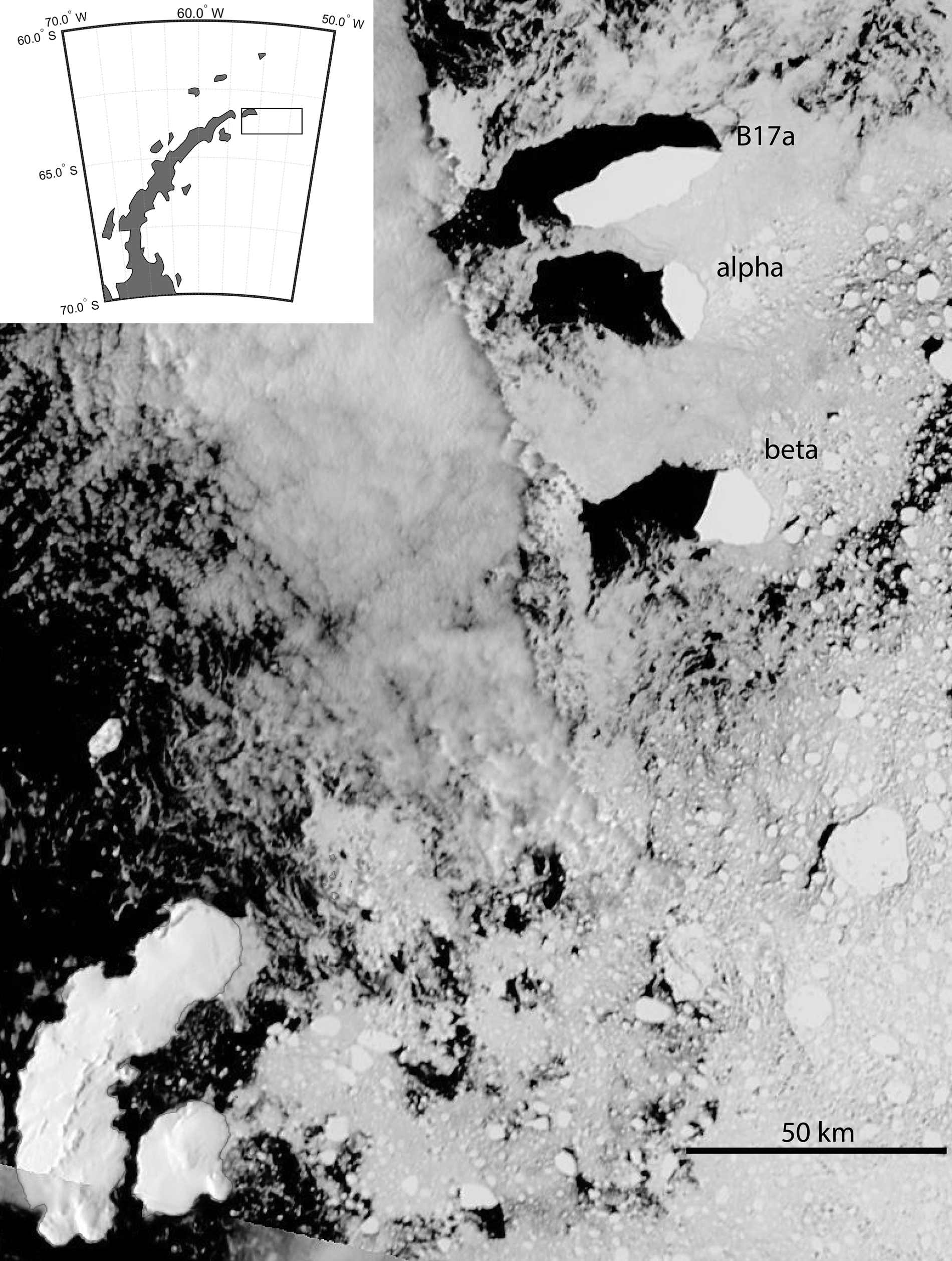
Fig. 1. Visible Aqua image from 23 February 2014 of the three large icebergs that are followed in this paper. From top to bottom-right are B17a and large icebergs labelled α and β, respectively. The inset shows the approximate area covered by the image north-east of the Antarctic Peninsula.
Data and methods
Tracking and size determination
A range of remote sensing tools were employed to track the three icebergs over their lifetimes following first detection in early March 2014. These included select images obtained by the Synthetic Aperture Radar instrument on Radarsat2, but also the MODIS Aqua and Terra visible imagery available through https://worldview.earthdata.nasa.gov/ on a daily basis. In addition, some positions of the largest iceberg, B17a, were provided through the National Oceanic and Atmospheric Administration (NOAA; http://www.natice.noaa.gov//pub/icebergs/Iceberg_Tabular.pdf), using their approximately weekly updated giant iceberg table, or the ASCAT and OSCAT2 giant iceberg altimetric positions provided several times a year at http://www.scp.byu.edu/current_icebergs.html. Whilst the resolution of these instruments and sources varies, the central position of each iceberg was able to be specified to within an accuracy of ~1 km.
Information about several size characteristics of each iceberg was evaluated from Radarsat2 images, as well as MODIS visible images where the entirety of an iceberg was cloud-free, using the Ice Tracking from SAR Images (ITSARI) segmentation algorithm (Silva & Bigg Reference Silva and Bigg2005). These shape parameters were the major axis and minor axis lengths, the perimeter and the iceberg area. It was found that the ITSARI algorithm was able to calculate these parameters to a precision of 0.1 km in analysis of the visible images, but it achieved a precision of closer to 0.01 km in the case of Radarsat2 images.
Meltwater impact
The impact of the meltwater from the icebergs on the surrounding water was assessed by examining the distribution of surface salinity in the region, as determined by the Aquarius satellite. This determined surface salinity by using three L-band microwave radiometers, with a sea surface temperature correction provided by other platforms and a wind speed correction provided by the scatterometer on board the satellite (Kao et al. Reference Braackmann-Folgmann, Shepherd, Gerrish, Izzard and Ridout2018). The data used were the Level-3 gridded data, available at a spatial resolution of 0.25° from https://podaac.jpl.nasa.gov/, so approximately equalling the spatial scale of the icebergs for much of their life. Weekly average data was extracted. The satellite failed in early June 2015, but it was operational throughout the lifetime of all three icebergs as they were tracked across the South Atlantic.
It is worth noting some limitations of the dataset. One of the radiometers did not work well at high latitudes, and the local presence of land or sea ice invalidates the salinity algorithm (Kao et al. Reference Kao, Lagerloef, Lee, Melnichenko, Meissner and Hacker2018). This will limit where salinity is available in our study, particularly when B17a was near islands or early in the icebergs' life history when they were near sea ice. However, the root mean square errors for the Level-3 data used were 0.13 practical salinity units (psu; Kao et al. Reference Kao, Lagerloef, Lee, Melnichenko, Meissner and Hacker2018), exceeding the mission specification of monthly means having an accuracy of better than 0.2 psu on a 150 km scale. Our study will suggest that these results are physically consistent well below the mission spatial scale aim.
Additional support for general surface-layer freshening in the vicinity of B17a is sought through selected Argo float profiles. Argo data are available via the Coriolis Data Assembly Centre (ftp://ftp.ifremer.fr/ifremer/argo), by geographical area (here, the Atlantic) and per float. By scrutinizing profile data in the vicinity of the icebergs during the latter half of 2014 and the first half of 2015, we identify two floats in the neighbourhood of B17a during April 2015, after this iceberg had drifted free from prolonged grounding near South Georgia. Table I provides the times and locations of Argo float profiles in April 2015, selecting all available data in the longitude range 33–37°W and latitude range 52–55°S. ‘Parked’ between profiles at a depth of 1000 m, both floats drift generally to the south-east during April: float 6901972 from 35.337°W, 52.785°S on 5 April to 34.692°W, 53.275°S on 25 April; and float 6902592 from 35.565°W, 52.038°S on 6 April to 34.105°W, 52.642°S on 26 April. Corresponding B17a locations during April 2015 are recorded in Table II. ‘Closest encounters’ are in late April, when both floats profile within 1° of longitude and latitude of B17a.
Table I. Times and locations for selected Argo float profiles in April 2015.

Table II. Locations of B17a during April 2015.

Productivity impact
The ocean productivity around the icebergs was assessed by the proxy of the surface chlorophyll a level, as observed by the MODIS ocean colour remotely sensed gridded dataset, using the OCI algorithm to produce chlorophyll a levels from radiometers on board the MODIS Aqua satellite (Hu et al. Reference Hu, Lee and Franz2012). This was available at daily temporal resolution, with a spatial resolution of 4 km, from the same NASA location from which the salinity data were obtained, over the same region of 40–65°S, 20–65°W. Many data are missing due to the extensive cloud cover over the Southern Ocean throughout the year.
Previous analyses of the impact of icebergs on Southern Ocean productivity have concentrated on short-term field measurements (e.g. Smith et al. Reference Smith, Sherman, Shaw, Murray, Vernet and Cefarelli2011), climatological mean relationships (e.g. Wu & Hou Reference Wu and Hou2017) or correlations over large datasets (e.g. Duprat et al. Reference Duprat, Bigg and Wilton2016). Here, however, we can follow the impacts of three large icebergs on productivity over 1 year or more.
In the analysis to follow, anomalies are shown, as well as absolute values. Due to the short lifetime of the Aquarius salinity instrument, monthly averages were computed for both salinity and surface chlorophyll a over 2012–2014 to maintain consistency between the analyses.
Iceberg modelling
An iceberg trajectory model was used here to simulate the paths of the three icebergs, forced by 3 hourly HYCOM ocean model currents and surface temperatures (https://www.hycom.org/; horizontal resolution 0.05°) and ECMWF ERA5 surface wind and air temperature fields (Copernicus Climate Change Service 2017; horizontal resolution 0.25°). The model originates from the Lagrangian particle approach developed by Bigg et al. (Reference Bigg, Wadley, Stevens and Johnson1997) and modified by Gladstone et al. (Reference Gladstone, Bigg and Nicholls2001), Levine & Bigg (Reference Levine and Bigg2008) and Bigg et al. (Reference Bigg, Cropper, O'Neill, Arnold, Fleming and Marsh2018). It models dynamical forces that move the icebergs and the thermodynamics that provide melting during transit. Whilst full details of the model formulation are provided in the above references, it is worth noting here that the dynamical forces affecting the individual icebergs are ocean, atmospheric and (if present) sea-ice drags, the Coriolis force, pressure gradients in the surrounding ocean and a wave radiation force. The dominant force tends to be the water drag, but, particularly in strong winds, other terms, such as the wave radiation stress and air drag, may become as important at times (Bigg et al. Reference Bigg, Wadley, Stevens and Johnson1997). In our simulations, sea ice is not present at any time due to the sea surface temperature always remaining above freezing point, so this force component is never applied. Note that icebergs may roll over if a stability criterion (Wagner et al. Reference Wagner, Stern, Dell and Eisenman2017) is not met. Note also that tides are not included in the HYCOM model forcing.
The thermodynamical processes contributing towards changing the mass of each iceberg are basal melting, buoyant convection, wave erosion, sublimation and latent heat transfer (Bigg et al. Reference Bigg, Wadley, Stevens and Johnson1997). Fracture is not included as a dynamic or thermodynamic process. In addition, if icebergs enter water shallower than their draught, then they ground and melt until their draught is reduced to below the local water depth. For simplicity of calculation, all icebergs simulated are rectangular in shape, with a width:length ratio of 1.0:1.5, this being similar to mean ratios found in both hemispheres. A ratio of draught to freeboard of 5:1 is assumed; again, this is more consistent with observations of the most common real icebergs of tabular and wedge shapes (Fequet Reference Fequet2002) than just assuming the buoyancy to be directly linked to the density difference between ice and seawater (for a full discussion of these ratios, see Bigg et al. Reference Bigg, Wadley, Stevens and Johnson1997). Again, for simplicity of calculation, all icebergs are assumed to be travelling with their long axes parallel to the surrounding water flow but with the atmospheric wind direction being 45° to the right of the iceberg. This is consistent with Ekman theory in the mean but will not always be the case in reality. As icebergs melt, their loss of mass is redistributed after calculation at each time step so as to maintain the ratios given above over time. Once modelled icebergs approach growler size (~5 m), they are assumed to instantaneously melt for numerical stability.
From a climatological perspective, previous iceberg modelling has been shown to lead to reasonable envelope predictions for iceberg presence in both the Southern Hemisphere (Gladstone et al. Reference Gladstone, Bigg and Nicholls2001, Martin & Adcroft Reference Martin and Adcroft2010, Marsh et al. Reference Marsh, Ivchenko, Skliris, Alderson, Bigg and Madec2015, Bigg et al. Reference Bigg, Cropper, O'Neill, Arnold, Fleming and Marsh2018) and Northern Hemisphere (Wilton et al. Reference Wilton, Bigg and Hanna2015, Marsh et al. Reference Marsh, Bigg, Zhao, Martin, Blundell and Josey2017). Even individual drift tracks can be reproduced in regions where forcing terms are well constrained and icebergs are assumed to be very thin (Bigg et al. Reference Bigg, Cropper, O'Neill, Arnold, Fleming and Marsh2018). Here, we present the first attempt to verify long-term iceberg trajectory modelling by comparing actual and modelled trajectories over timescales of weeks to months. However, as will be seen in the next section, knowledge of the key iceberg parameters of major and minor axes is only intermittently available, and estimates of iceberg depth are essentially non-existent. Similarly, the next section also demonstrates that errors in simulated tracks due to these poor initial conditions quickly grow to the point where a continuous simulation for the whole lifetime of each iceberg would be uninformative. Simulation of only monthly track segments is therefore done, with resetting of the surviving icebergs' initial conditions in the model at the beginning of each calendar month, from March 2014 until May 2015. The estimates of major and minor axes for the start of each month are used as model initial conditions to give a measure of the uncertainty in the track due to size errors; these are denoted as the ‘regular’ (REG) simulations. Note that whilst the modelled icebergs are sometimes larger than the ocean model forcing, they are not larger than the atmospheric forcing grid. Thus, for simplicity, the decision was taken to use the ocean and atmospheric forcing as interpolated to the central point of each modelled iceberg. Given the uncertainty in iceberg size (also see below) and the fact that this work represents the first attempt at this approach, this limitation needs to be kept in mind.
The lack of knowledge of iceberg depths is addressed by running a suite of ensembles for each monthly segment with combined aerial and submarine depths of 100, 200, 300 and 400 m, respectively; these are denoted the ‘depth’ (DEP) simulations. In DEP simulations, the minor axis size estimate is taken as the iceberg width. Note that as B17a was grounded off South Georgia in water ~270–300 m deep at its shallowest, the 100 m DEP simulation for B17a was not used until April 2015, by which time B17a had freed itself. Note also that all monthly simulations start with an assumption of zero velocity, but if a giant iceberg has a significant initial velocity that changes the momentum through modelling from rest, there will be a cumulative offset in the predicted position. In addition, for simplicity, we use the surface ocean forcing fields to drive the model. One could improve this in the future if one had confidence in the reliability of the vertical profile of an ocean model in a region of limited assimilated data.
Results
Here, we examine the physical evolution of the triplet of large icebergs, along with their influences on the local ocean salinity and primary productivity, as well as a study of attempting to model the icebergs' movements. Due to the multiple approaches used, we here combine a measure of discussion in each separate sub-section, as well as a strict presentation of the results. The novelty of this study's combined system approach requires this atypical structure. An integration of the various components is then given in the following ‘Discussion’ section.
Evolution of the large iceberg triplet across the South Atlantic
Despite the three icebergs leaving the Weddell Sea in late February 2014 and starting from within a few kilometres of each other (Fig. 1), they followed very different paths across the South Atlantic after the first few weeks, surviving for time periods between just under 1 year (iceberg α) to almost 15 months (B17a), whilst travelling between 1750 (B17a) and 3000 (α) km. Their relative paths are shown in Fig. 2, with the individual positions of observations for each iceberg given in the ‘Tracks&Images’ spreadsheet in the Supplementary Material. It is worth noting the seemingly linear excursion of B17a in Fig. 2, near 58°S. This is due to a sequence of daily observations providing more detail of the iceberg's short-term trajectory. Here, Fig. 2 shows B17a trapped in a large eddy (Fig. 3), which must be at least several hundred metres deep. Typically, there were periods of 1–2 weeks between observations of each iceberg, so a daily sequence is atypical.

Fig. 2. Tracks of three large icebergs from 6 March 2014 until their break-up. Icebergs are B17a (solid line; ‘+’), α (dotted line; ‘×’) and β (dashed line; ‘o’) - all start at approximately the same location off the Antarctic Peninsula. Markers are shown on each track approximately every 3 months to give a sense of relative speed.

Fig. 3. Anomalous Aviso altimetric height for August 2014, showing the eddy in which B17a was trapped for several days. The path of B17a is shown in black from mid-July to mid-August using data from the Argo Global Marine Atlas (https://argo.ucsd.edu/data/data-visualizations/marine-atlas/).
B17a also experienced significant periods of partial grounding near two islands. In the first half of May 2014, for ~2 weeks, B17a remained off the east coast of Clarence Island (61.20°S, 54.08°W), the easternmost island of the South Shetland Islands chain. At this time, the iceberg was over half as big again as the island's longest axis, and the combination of this size and the rapid deepening of the narrow shelf around the island meant that B17a was not fully grounded. Its narrow end collided with the shelf at the southern end of Clarence Island, and the currents swung the iceberg clockwise until it was parallel to Clarence Island's east coast, at which point it rapidly moved away northwards. B17a had a much longer period of grounding off south-west South Georgia (~55.18°S, 36.33°W), where it remained for ~5 months, from early November 2014 to late March 2015. The iceberg remained fixed and static for much of this time, with some initial slow oscillation of its western end until it became firmly grounded. Eventually, the impact of the differential stress gradient between the grounded and free-floating parts of B17a meant it experienced major fracturing at one end (Fig. 4), first splitting in two (Fig. 4a) and then the smaller segment fragmenting into a number of significant but much smaller icebergs (Fig. 4b), freeing the main body of the iceberg to finally move around the southern end of the island (Fig. 2). However, it is worth noting that 2 months earlier, in late January 2015, some minor fracturing had led to a few small icebergs breaking off B17a and moving shorewards.

Fig. 4. The end of B17a's grounding south of the island of South Georgia. a. Radarsat2 SAR image from 14 March 2015. b. MODIS Aqua visible image from 16 March 2015.
As confirmed by the visual inspection of each available visual or synthetic aperture radar (SAR) image, such cracking and shedding of smaller but substantial icebergs were only occasional features of all three icebergs' histories, and these were mainly confined to the last stages of the icebergs' lives, except in the interactions of B17a with islands. The dimensions of the icebergs, as determined by the ITSARI analysis, therefore tended to evolve only slowly, as mass was mostly loss due to melting rather than fracture (Fig. 5). This to some extent contradicts Bouhier et al.'s (Reference Bouhier, Tournadre, Rémy and Gourves-Cousin2018) reliance on fragmentation as a contribution to mass loss for giant icebergs (including B17a) in open waters. However, their data (Bouhier et al. Reference Bouhier, Tournadre, Rémy and Gourves-Cousin2018, fig. 11) also indicate this fracture mechanism to be strongest in the last few months of an iceberg's lifetime. Fracture events also significantly change the remaining iceberg's speed, leading to short-term increases in speed as the accelerating force terms exerted by the ocean on the iceberg (Bigg et al. Reference Bigg, Wadley, Stevens and Johnson1997) change abruptly. This can be seen in Fig. 6 towards the end of each iceberg's lifetime. It is worth noting, however, that there tends to be a quasi-periodic oscillation in each iceberg's speed, with peaks separated by periods of 20–50 days. As the peaks are sometimes at similar times for different icebergs, this is probably a reflection of similar variability in the large-scale Southern Ocean wind field in the area (as can be seen in Lin Reference Lin2018, fig. 1), transmitted into changes in ocean currents. Despite the short-term variability, all three icebergs had similar mean speeds over their open-water lifetimes (~15 ± 12 cm s-1), comparable to the mean surface ocean current (Bouhier et al. Reference Bouhier, Tournadre, Rémy and Gourves-Cousin2018). Nevertheless, there is a trend towards higher speeds over the last 3 months of the lifetimes of bergs α and β and in the post-grounding life of B17a (Fig. 6). This is a reflection of the basal melting of the icebergs, reducing their depth (Bouhier et al. Reference Bouhier, Tournadre, Rémy and Gourves-Cousin2018) and so allowing the water drag on the iceberg to be controlled more by the faster surface currents, as well as allowing atmospheric drag from the winds to play a relatively larger role in iceberg dynamics (Bigg et al. Reference Bigg, Wadley, Stevens and Johnson1997).

Fig. 5. Key shape parameters and their variation over time for each iceberg: a. major axis length, b. minor axis length, c. perimeter and d. area. All values derive from application of the ITSARI algorithm on either SAR (Radarsat2) images (solid lines) or MODIS visible imagery (dashed lines).

Fig. 6. The temporal variation in the speed of the three icebergs. The periods of low speeds for B17a at approximately day 110 and at the turn of 2014–2015 occurred when the iceberg was grounded.
Changes in some key shape parameters over the lifetime of the three icebergs are shown in Fig. 5. Concentrating on the much higher-resolution SAR imagery, the slow evolution of all aspects of the icebergs' shapes is seen clearly. The larger iceberg, B17a, which had a longer-term history of earlier fracture events in the sea-ice region around Antarctica (Bouhier et al. Reference Bouhier, Tournadre, Rémy and Gourves-Cousin2018), loses mass more quickly, but still relatively slowly until the freeing of the iceberg from its grounding off South Georgia in March 2015. It is noteworthy that using MODIS visual imagery to calculate spatial parameters with the semi-automatic algorithm ITSARI (Silva & Bigg Reference Silva and Bigg2005) gives a much more temporally variable pattern for all shape parameters, with both a 30% higher offset and high variance from one image to another.
At the end of the large icebergs' lives, they break up into multiple pieces: B17a split into five large fragments, iceberg α into three fragments, whilst iceberg β split into six fragments, all being > 1 km in some dimension. However, icebergs of this size become very sensitive to melting and fragmentation caused by the rough seas of the Southern Ocean, and the fragments disappear within a few days at most.
Influence of the large icebergs on the local salinity field
Both the size of B17a and its relatively large change over time (Fig. 5) suggest that this iceberg would have had a larger impact on ocean salinity than that caused by bergs α and β. Unfortunately, the degrading of the Aquarius signal due to the proximity to sea ice and the high latitude from which the icebergs start their journey mean that it is not until well into the spring of 2014 that Aquarius recorded salinity data in the vicinity of the icebergs. B17a and iceberg β approached 55°S before this was possible, whilst iceberg α was near an anomalous northwards extension of sea ice in the Weddell Gyre (see archives at https://nsidc.org/data/seaice_index) until early December 2014.
Nevertheless, once salinity data are available, the impact of iceberg melting is visible. The instantaneous response of surface salinity to the melting icebergs is seen in Fig. 7a, which does indeed show a larger freshening impact from the bigger iceberg B17a. The smaller icebergs do not show a clear mean freshening signal because of the high noise in the local means due to the short period from which the background monthly mean is calculated. However, more noticeable is the longer-term impact on salinity (Fig. 7b). All of the icebergs are associated with a statistically significant decrease in the mean salinity 1 month after the iceberg has passed by - their basal melting gives a sustained plume of fresher water behind the iceberg. The magnitude of this freshening is temporally variable, but it averages at ~0.5 psu for each iceberg, although it can, in the short term, lead to freshening of up to 2 psu (Fig. 7b).

Fig. 7. Surface salinity anomaly averaged over the 1° square around the position of each iceberg's centre a. in the week of the iceberg's presence and b. 4 weeks later. The monthly anomalies are calculated from the relatively short-lived Aquarius mission. Note that the B17a peak in b. is an artefact of the poorer remote sensing signal due to the lengthy grounding of the iceberg.
An integral measure of freshening in the vicinity of B17a, late in its drift, is suggested in the selected Argo profiles. Figure 8 presents temperature and salinity profiles over January–June 2015 sampled by Argo floats 6901972 and 6902562. Each float provides three profiles during April, at locations indicated by blue star symbols in the accompanying maps in Fig. 8. The longer time span provides some seasonal context, as both floats sample a mixed layer of depth 50–100 m (defined where potential density exceeds 0.1 of the surface value), which cools and deepens into winter. As B17a drifts to the north-east, into the vicinity of these two floats, there is some evidence for mixed-layer freshening of 0.05–0.10 psu before/during April. Of the two floats, the stronger fresh signal recorded by float 6902562 (Fig. 8, lower left panel) is consistent with profiling to the north and east of B17a, probably linked to eastward drift of meltwater in the ACC; the weaker fresh signal recorded by float 6901972 (Fig. 8, second left panel) may be a consequence of profiling further to the south and west, and hence peripheral sampling of the B17a meltwater plume.

Fig. 8. Temperature and salinity profiles over January–June 2015 sampled by Argo floats 6901972 and 6902562, selected for proximity to B17a during April 2015 (highlighted by red boxes in the profile data), specifying mixed-layer depth (black line) where the potential density falls to < 0.1 kg m-3 of the uppermost value; each float provides three profiles during April at locations indicated by blue star symbols in the accompanying maps, also indicating the local trajectory of B17a (see Tables I & II for further details).
Impact of iceberg meltwater on ocean productivity
The clear meltwater signal associated with each iceberg shown in Fig. 7 is expected to lead to a significant impact on ocean productivity around and in the plume stemming from each iceberg. The meltwater will contain nutrients and trace micronutrients such as iron, encouraging production, and this effect will have been enhanced by the entrainment of nutrients from deeper in the water column via the rising basal melt plume (Smith et al. Reference Smith, Sherman, Shaw and Sprintall2013). However, the notable temporal variability in the freshening signal shown in Fig. 7 and particularly the longer-term perspective seen in Fig. 7b suggest that this productivity enhancement will also be variable over time.
Figure 9 shows the chlorophyll a anomaly in the 3° × 3° square around cloud-free observations for each of the three icebergs. Where anomalies relative to the previous month exceed those relative to the current month, we infer that the iceberg has enhanced primary production. This demonstrates significant variability over time, as implied by the freshening signal, with the larger iceberg, B17a, having the largest impact in terms of producing positive chlorophyll a anomalies (Fig. 9a). This iceberg, and to a lesser extent iceberg β, showed a bigger impact on the chlorophyll a signal compared to 1 month earlier. There is a similar but variable impact 1 month later.

Fig. 9. Chlorophyll a (chla) anomalies in the 3° × 3° square around each iceberg's location, showing anomalies relative to the current month (+) and the previous month (*): a. B17a, b. iceberg α and c. iceberg β. Note that there needs to be at least one daily observation of the sea surface (i.e. without obscuring clouds) within the square for the comparison to be possible.
Whilst the above spatially averaged and, to some extent, time averaged analyses are suggestive of freshening and chlorophyll a relationships associated with large icebergs, they do not give a firm statistical signal. However, it is clear from previous analyses (e.g. Duprat et al. Reference Duprat, Bigg and Wilton2016) that large icebergs have distinctive and spatially variable chlorophyll a plumes extending from them. The relatively few occasions when either MODIS Aqua or Terra chlorophyll a sensors saw entire icebergs and sufficient surrounding cloud-free water to enable an estimate of chlorophyll a and salinity levels were therefore extracted. There were 24 days when B17a was visible in this way, 13 occasions for iceberg α and 14 for iceberg β (see the ‘Tracks&Images’ spreadsheet in the Supplementary Material). The mean 3° × 3° salinity anomalies were -0.39, 0.04 and -0.19 psu, with 83%, 60% and 83% days, respectively, with negative salinity anomalies for B17a, iceberg α and iceberg β. These figures represent majorities for all three icebergs and almost all for B17a and iceberg β. Only iceberg α, which spent most of its life in colder waters further south than either of the other two (Fig. 2), did not have a dominant freshening signal during the times when a visible image could be obtained.
The presence of spatially uneven chlorophyll a plumes means that there is not a significant correlation between the 3° × 3° chlorophyll a and salinity anomalies for the visible images for any of the three icebergs. However, many of the plumes showed areas with enhanced chlorophyll a above the mean background level of 0.2 mg m-3 (Duprat et al. Reference Duprat, Bigg and Wilton2016). Of the three icebergs, 15 of the B17a, 4 of the α and 11 of the β images showed chlorophyll a levels in at least one sector around the respective iceberg with a > 50% enhancement above this level. In some cases, for each iceberg, this anomalously high chlorophyll a level was over an order of magnitude above the long-term mean. Example chlorophyll a plumes for each iceberg are shown in Fig. 10.

Fig. 10. Worldview chlorophyll a plumes associated with each iceberg: a. B17a (Terra, 23 January 2015), b. α (Aqua, 14 December 2014) and c. β (Aqua, 8 January 2015). The position of the iceberg is marked on each image.
Modelling of iceberg movement
Figures 11 & 12 show the REG and DEP model simulations for the three icebergs. These show clearly that variation in the estimated depth of an iceberg leads to a much bigger envelope of model evolutions over 1 month than differences in major axes imposed within the REG simulations. Typically, the horizontal dimensions are relatively well known, and Fig. 11 shows that, in most examples, a 20–30% difference in initial horizontal dimension allows simulations to evolve similarly for ~2 weeks, despite the high temporal and spatial resolution of the forcing fields. However, keeping the same horizontal dimensions but allowing depth to vary by a factor of 4 leads to rapid divergence of simulations (Fig. 12) due to the force terms being mostly depth dependent (Bigg et al. Reference Bigg, Wadley, Stevens and Johnson1997).

Fig. 11. REG iceberg model simulations for icebergs a. α, b. β and c. B17a. Each pair of simulations starts on the first day of successive months, from March 2014 to March 2015. Red and blue lines are for initializations using major and minor iceberg axes estimates, respectively.

Fig. 12. DEP iceberg model simulations for icebergs a. α, b. β and c. B17a. Each set of simulations starts on the first day of successive months, from March 2014 to March 2015. Green, red, black and blue lines are for initializations using depths of 100, 200, 300 and 400 m, respectively. In the case of B17a, the simulations run to May 2015 and only the 200 and 300 m depth models are shown, in red and blue, respectively.
However, Figs 11 & 12 also show the limitations of attempting to predict the motion of giant icebergs. Limited knowledge of the actual dimensions of a giant iceberg, particularly its depth and whether this is uniform across the iceberg, is a fundamental limitation for prediction in practice. In addition, in the remote areas where icebergs are found in the Southern Ocean, the accuracy of the ocean and atmospheric model reanalyses on which the forcing terms are based is poor, especially in the late autumn to early spring, when there is little ground truthing available due to persistent cloud cover, darkness and limited direct observations. Thus, even for B17a, whose grounding off South Georgia meant that its depth was very likely to be in the order of 200–300 m, corresponding to the bathymetry in the region, the combination of forcing and initial size constraints meant that prediction had limited success (Fig. 12c).
Figure 13 represents the best tool to assess the accuracy of the modelling experiments. Figure 13 plots the differences between the simulations and actual positions for the few months with at least 5 days of direct visual or SAR observation of icebergs β and B17a. Figure 13 suggests that positional errors mostly remain < 200 km for the first 2 weeks of a simulation, but that by the end of 1 month positional errors are likely to be substantially larger. However, when considering the full month of the comparison, both simulations can be used to infer probable depths. Therefore, simulations for iceberg β (Fig. 13a) appear to be best for the 100 m-depth assumption, whilst B17a's 300 m simulations (Fig. 13b) have lower errors than the 200 m ones, which is consistent with the South Georgia bathymetry, where grounding occurs for an extensive period.

Fig. 13. Differences between observed and model locations for DEP simulations of icebergs a. β and b. B17a for those months with at least five dates with visual or SAR observations to confirm the icebergs' locations. Green, red, black and blue lines are for initializations using depths of 100, 200, 300 and 400 m, respectively. Iceberg α only had two months with sufficient data and is not shown.
Discussion
There are clear limitations to this study because of the difficulty in gathering reliable data regarding even large icebergs in the Southern Ocean. Clouds frequently obscure their surfaces, particularly in the late autumn and winter, preventing the collection of chlorophyll a data. The high latitudes and the presence of sea ice quite far north, particularly in the late autumn to early spring, make the collection of remotely sensed salinity and velocity data variable. Even the collection of high-resolution SAR data for size assessment is variable - if the desired iceberg target is some distance from land, a special advance request to activate the capture of an image is required. Nevertheless, sufficient data have been gathered to characterize the three icebergs, their divergence over time and their freshwater and chlorophyll a impact on the surrounding ocean, these latter two from spring to autumn during the icebergs' melting. Further ‘data of opportunity’ are identified where two Argo floats provide serendipitous profiles in the close vicinity of B17a, to the north-east of South Georgia, sampling relatively low salinity throughout a mixed layer of ~100 m in vertical extent.
The three large icebergs exited the Weddell Sea within a few kilometres of each other in March 2014 (Fig. 1). They moved north-east at a similar rate for ~3 months (Fig. 2) but then began to diverge significantly whilst still all travelling in a north-east direction. A measure of their dispersion is shown in Fig. 14. This clearly shows the difference between open ocean dispersion and times when interaction with islands is dominant. Early in the record, divergence actually decreases as B17a collided with Clarence Island and iceberg β also interacted with the local island chain. From approximately Julian Day 150 through to approximately Julian Day 250, the icebergs spread apart as they joined the ACC, although B17a and iceberg β followed a similar trajectory, minimizing the overall dispersion. Over the next couple of months, all of the icebergs slowed, causing convergence, as they approached South Georgia, which blocks the ACC, diverting the main current northwards. Once B17a was grounded south-west of South Georgia, the divergence increased rapidly in the short term as icebergs α and β moved away. However, these two icebergs began to converge into the main ACC downstream, reducing divergence again, even though B17a was still grounded. The monotonically increasing convergence seen by Corrado et al. (Reference Corrado, Lacorata, Palatella, Santoleti and Zambianchi2017) in the drifter field of the Southern Ocean is therefore not followed by the iceberg triplet, whose divergence is controlled by local land-iceberg interaction and the regional convergence under the influence of the ACC in the South Atlantic.

Fig. 14. Dispersion of the iceberg triplet over their common lifetime.
The iceberg triplet had a distinct but temporally highly variable impact on the surrounding ocean. Whilst the first winter of the icebergs' travels in the Southern Ocean cannot be studied due to limitations in the remote sensing tools available, it is clear from later seasons that B17a, as the larger iceberg, being initially double the area of either iceberg α or β, has a larger impact on ocean salinity and productivity.
Are these salinity signals consistent with a meltwater plume in the wake of B17a that is vertically mixed throughout the mixed layer? Consider a change of mixed layer salinity, ΔS, generally equated to a freshwater flux, P − E + R (units m s-1, positive into the ocean) due to the balance between precipitation (P), evaporation (E) and runoff (R; see Equation 1):
 $$P-E + R = {-}h\displaystyle{1 \over {S_0}}\displaystyle{{\Delta S} \over {\Delta t}}$$
where S 0 is a representative salinity (35 psu), t is time and h is mixed-layer depth. Multiplication by -1 converts a salinity increase (decrease) to a freshwater loss (gain). Identifying salinity change with the runoff (meltwater) term alone, sustained for 1 month at a given location (subject to the freshwater plume), and assuming a mixed-layer depth of 100 m, a change of 0.1 psu implies a flux of 1.1 × 10⁻⁷ m s-1, or 3.5 m year-1. This is consistent with a background rate of ~0.5 m year-1 for year-round iceberg melting in this region, obtained with coupled ocean-iceberg models (e.g. Marsh et al. Reference Marsh, Ivchenko, Skliris, Alderson, Bigg and Madec2015). When further noting the surface salinity anomalies of 0.5–1.0 psu detected in Aquarius data, the implication is that meltwater close to the melting iceberg exists near the surface as a cold and fresh surface sublayer. For consistency with salinity anomalies of 0.05–0.10 psu throughout a mixed layer of depth 100 m, the fresher surface layer would be of depth 5–10 m.
Thus, in general, in the case of the salinity anomaly caused by the large icebergs, this can be as much as a freshening of several psu, with evidence, as argued above, of mixing throughout an autumn mixed layer of ~100 m depth and an implied meltwater flux that is consistent with model estimates for the region. However, all of the icebergs exhibit longevity in their impact, with a discernible freshening discernible up to 1 month later (Fig 7 & 8).
The freshening impact from the slow but continual melting (Fig. 5) is sustained, whilst the impact of this meltwater on ocean productivity is much more episodic (Fig. 9). This productivity effect is also larger and more frequent for B17a than is the case for the other two icebergs, but they all show strong temporal variability in chlorophyll a enhancement. This is usually stronger 1 month later (Fig. 9). There is nevertheless only a poor correlation between the freshening and productivity changes. This contrast in physical and biological impacts on the surrounding waters means that modelling the long-term impacts of large icebergs on polar waters will be more straightforward for the physical than biological components. Both, however, show significant variability that will not be accurately captured by current iceberg melt models (e.g. Bigg et al. Reference Bigg, Wadley, Stevens and Johnson1997, Marsh et al. Reference Marsh, Ivchenko, Skliris, Alderson, Bigg and Madec2015, Bouhier et al. Reference Bouhier, Tournadre, Rémy and Gourves-Cousin2018) beyond ~2 weeks into the future. However, our modelling experiments have shown that current iceberg modelling can be used for larger icebergs reasonably well in the short term, but this analysis also suggests that if giant iceberg trajectories need to be predicted in regions of highly variable currents, such as the outflow from the Weddell Gyre, a highly monitored environment is a prerequisite. Modelling may also represent a tool for investigating the probable depths of icebergs where this information is not known.
Conclusion
This paper has demonstrated that large icebergs survive for many months within the Southern Ocean and have a physical and biological impact on the surface layer of the local ocean for distances of up to hundreds of kilometres away, persisting for weeks to 1 month. However, both the physical freshening impact of the meltwater and particularly its fertilizing effect on the surrounding ocean are highly variable over time. Whilst modelling the physical impacts may be feasible using daily or sub-daily forcing (for a theoretical study relevant to this, see Bigg et al. Reference Bigg, Cropper, O'Neill, Arnold, Fleming and Marsh2018), explaining the biological impacts, and therefore calculating the impact of large iceberg fertilization on ocean carbon storage, is likely to remain problematic, especially given the difficulties found with modelling iceberg trajectories over longer timescales. Approximate estimates of carbon storage, such as those of Duprat et al. (Reference Duprat, Bigg and Wilton2016), may be all that is feasible for some time.
Acknowledgements
We would like to thank Rebekah Stanton, who carried out some initial collection of chlorophyll a data in the first few months of 2015 as a volunteer part-time researcher at the University of Sheffield. Argo data were collected and made freely available by the International Argo Program and the national programmes that contribute to it (http://www.argo.ucsd.edu, http://argo.jcommops.org); the Argo Program is part of the Global Ocean Observing System. We would also like to thank the anonymous reviewers for their comments.
Author contributions
GRB designed the analysis and carried out the tracking, modelling and analysis of the salinity and chlorophyll a data. He coordinated the writing of the manuscript. RM accessed, plotted and analysed the Argo float data and contributed to the manuscript.
Financial support
Aspects of the original monitoring and modelling of the triplet of icebergs were funded by the Natural Environmental Research Council through grant NE/M007820/1 ‘Iceberg forecasting - from days to decades (ICECAST)’.
Supplemental material
Two supplemental tables will be found at https://doi.org/10.1017/S0954102022000517.


