


1. Introduction
With the exponential growth in the amount of available textual resources, organization, categorization, and summarization of these data presents a challenge, the extent of which becomes even more apparent when it is taken into account that a majority of these resources do not contain any adequate meta information. Manual categorization and tagging of documents is unfeasible due to a large amount of data, therefore, development of algorithms capable of tackling these tasks automatically and efficiently has become a necessity (Firoozeh et al. Reference Firoozeh, Nazarenko, Alizon and Daille2020).
One of the crucial tasks for organization of textual resources is keyword identification, which deals with automatic extraction of words that represent crucial semantic aspects of the text and summarize its content. First automated solutions to keyword extraction have been proposed more than a decade ago (Witten et al. Reference Witten, Paynter, Frank, Gutwin and Nevill-Manning1999; Mihalcea and Tarau Reference Mihalcea and Tarau2004) and the task is currently again gaining traction, with several new algorithms proposed in the recent years. Novel unsupervised approaches, such as RaKUn (Škrlj, Repar, and Pollak Reference Škrlj, Repar and Pollak2019) and YAKE (Campos et al. Reference Campos, Mangaravite, Pasquali, Jorge, Nunes and Jatowt2018), work fairly well and have some advantages over supervised approaches, as they are language and genre independent, do not require any training and are computationally undemanding. On the other hand, they also have a couple of crucial deficiencies:
-
• Term frequency–inverse document frequency (TfIdf) and graph-based features, such as PageRank, used by these systems to detect the importance of each word in the document, are based only on simple statistics like word occurrence and co-occurrence, and are therefore unable to grasp the entire semantic information of the text.
-
• Since these systems cannot be trained, they cannot be adapted to the specifics of the syntax, semantics, content, genre and keyword assignment regime of a specific text (e.g., a variance in a number of keywords).
These deficiencies result in a much worse performance when compared to the state-of-the-art supervised algorithms (see Table 2), which have a direct access to the gold-standard keyword set for each text during the training phase, enabling more efficient adaptation. Most recent supervised neural algorithms (Chen et al. Reference Chen, Zhang, Wu, Yan and Li2018; Meng et al. Reference Meng, Yuan, Wang, Brusilovsky, Trischler and He2019; Yuan et al. Reference Yuan, Wang, Meng, Thaker, Brusilovsky, He and Trischler2020), therefore, achieve excellent performance under satisfactory training conditions and can model semantic relations much more efficiently than algorithms based on simpler word frequency statistics. On the other hand, these algorithms are resource demanding, require vast amounts of domain-specific data for training, and can therefore not be used in domains and languages that lack manually labeled resources of sufficient size.
In this research, we propose Transformer-Based Neural Tagger for Keyword IDentification (TNT-KID)Footnote a that is capable of overcoming the aforementioned deficiencies of supervised and unsupervised approaches. We show that while requiring only a fraction of manually labeled data required by other neural approaches, the proposed approach achieves performance comparable to the state-of-the-art supervised approaches on test sets for which a lot of manually labeled training data are available. On the other hand, if training data that is sufficiently similar to the test data are scarce, our model outperforms state-of-the-art approaches by a large margin. This is achieved by leveraging the transfer learning technique, where a keyword tagger is first trained in an unsupervised way as a language model on a large corpus and then fine-tuned on a (usually) small-sized corpus with manually labeled keywords. By conducting experiments on two different domains, computer science articles and news, we show that the language model pretraining allows the algorithm to successfully adapt to a specific domain and grasp the semantic information of the text, which drastically reduces the needed amount of labeled data for training the keyword detector.
The transfer learning technique (Peters et al. Reference Peters, Neumann, Iyyer, Gardner, Clark, Lee and Zettlemoyer2018; Howard and Ruder Reference Howard and Ruder2018), which has recently become a well-established procedure in the field of natural language processing (NLP), in a large majority of cases relies on very large unlabeled textual resources used for language model pretraining. For example, a well-known English BERT model (Devlin et al. Reference Devlin, Chang, Lee and Toutanova2019) was pretrained on the Google Books Corpus (Goldberg and Orwant Reference Goldberg and Orwant2013) (800 million tokens) and Wikipedia (2500 million tokens). On the other hand, we show that smaller unlabeled domain-specific corpora (87 million tokens for computer science and 232 million tokens for news domain) can be successfully used for unsupervised pretraining, which makes the proposed approach easily transferable to languages with less textual resources and also makes training more feasible in terms of time and computer resources available.
Unlike most other proposed state-of-the-art neural keyword extractors (Meng et al. Reference Meng, Zhao, Han, He, Brusilovsky and Chi2017, Reference Meng, Yuan, Wang, Brusilovsky, Trischler and He2019; Chen et al. Reference Chen, Zhang, Wu, Yan and Li2018; Ye and Wang Reference Ye and Wang2018; Yuan et al. Reference Yuan, Wang, Meng, Thaker, Brusilovsky, He and Trischler2020), we do not employ recurrent neural networks but instead opt for a transformer architecture (Vaswani et al. Reference Vaswani, Shazeer, Parmar, Uszkoreit, Jones, Gomez, Kaiser and Polosukhin2017), which has not been widely employed for the task at hand. In fact, the study by Sahrawat et al. (Reference Sahrawat, Mahata, Kulkarni, Zhang, Gosangi, Stent, Sharma, Kumar, Shah and Zimmermann2020) is the only study we are aware of that employs transformers for the keyword extraction task. Another difference between our approach and most very recent state-of-the-art approaches from the related work is also task formulation. While Meng et al. (Reference Meng, Zhao, Han, He, Brusilovsky and Chi2017), (Reference Meng, Yuan, Wang, Brusilovsky, Trischler and He2019) and Yuan et al. (Reference Yuan, Wang, Meng, Thaker, Brusilovsky, He and Trischler2020) formulate a keyword extraction task as a sequence-to-sequence generation task, where the classifier is trained to generate an output sequence of keyword tokens step by step according to the input sequence and the previous generated output tokens, we formulate a keyword extraction task as a sequence labeling task, similar as in Gollapalli, Li, and Yang (Reference Gollapalli, Li and Yang2017), Luan, Ostendorf, and Hajishirzi (Reference Luan, Ostendorf and Hajishirzi2017) and Sahrawat et al. (Reference Sahrawat, Mahata, Kulkarni, Zhang, Gosangi, Stent, Sharma, Kumar, Shah and Zimmermann2020).
Besides presenting a novel keyword extraction procedure, the study also offers an extensive error analysis, in which the visualization of transformer attention heads is used to gain insights into inner workings of the model and in which we pinpoint key factors responsible for the differences in performance of TNT-KID and other state-of-the-art approaches. Finally, this study also offers a systematic evaluation of several building blocks and techniques used in a keyword extraction workflow in the form of an ablation study. Besides determining the extent to which transfer learning affects the performance of the keyword extractor, we also compare two different pretraining objectives, autoregressive language modeling and masked language modeling (Devlin et al. Reference Devlin, Chang, Lee and Toutanova2019), and measure the influence of transformer architecture adaptations, a choice of input encoding scheme and the addition of part-of-speech (POS) information on the performance of the model.
The paper is structured as follows. Section 2 addresses the related work on keyword identification and covers several supervised and unsupervised approaches to the task at hand. Section 3 describes the methodology of our approach, while in Section 4 we present the datasets, conducted experiments and results. Section 5 covers error analysis, Section 6 presents the conducted ablation study, while the conclusions and directions for further work are addressed in Section 7.
2. Related work
This section overviews selected methods for keyword extraction, supervised in Section 2.1 and unsupervised in Section 2.2. The related work is somewhat focused on the newest keyword extraction methods, therefore, for a more comprehensive survey of slightly older methods, we refer the reader to Hasan and Ng (Reference Hasan and Ng2014).
2.1 Supervised keyword extraction methods
Traditional supervised approaches to keyword extraction considered the task as a two step process (the same is true for unsupervised approaches). First, a number of syntactic and lexical features are used to extract keyword candidates from the text. Second, the extracted candidates are ranked according to different heuristics and the top n candidates are selected as keywords (Yuan et al. Reference Yuan, Wang, Meng, Thaker, Brusilovsky, He and Trischler2020). One of the first supervised approaches to keyword extraction was proposed by Witten et al. (Reference Witten, Paynter, Frank, Gutwin and Nevill-Manning1999), whose algorithm named KEA uses only TfIdf and the term’s position in the text as features for term identification. These features are fed to the Naive Bayes classifier, which is used to determine for each word or phrase in the text if it is a keyword or not. Medelyan, Frank, and Witten (Reference Medelyan, Frank and Witten2009) managed to build on the KEA approach and proposed the Maui algorithm, which also relies on the Naive Bayes classifier for candidate selection but employs additional semantic features, such as, for example, node degree, which quantifies the semantic relatedness of a candidate to other candidates, and Wikipedia-based keyphraseness, which is the likelihood of a phrase being a link in the Wikipedia.
Wang, Peng, and Hu (Reference Wang, Peng and Hu2006) was one of the first studies that applied a feedforward neural network classifier for the task at hand. This approach still relied on manual feature engineering and features such as TfIdf and appearance of the keyphrase candidate in the title or heading of the given document. On the other hand, Villmow, Wrzalik, and Krechel (Reference Villmow, Wrzalik and Krechel2018) applied a Siamese Long Short-Term Memory (LSTM) network for keyword extraction, which no longer required manual engineering of statistical features.
A more recent supervised approach is the so-called sequence labeling approach to keyword extraction by Gollapalli et al. (Reference Gollapalli, Li and Yang2017), where the idea is to train a keyword tagger using token-based linguistic, syntactic and structural features. The approach relies on a trained Conditional Random Field (CRF) tagger and the authors demonstrated that this approach is capable of working on-par with slightly older state-of-the-art systems that rely on information from the Wikipedia and citation networks, even if only within-document features are used. In another sequence labeling approach proposed by Luan et al. (Reference Luan, Ostendorf and Hajishirzi2017), a sophisticated neural network is built by combing an input layer comprising a concatenation of word, character and part-of-speech embeddings, a bidirectional Long Short-Term Memory (BiLSTM) layer and, a CRF tagging layer. They also propose a new semi-supervised graph-based training regime for training the network.
Some of the most recent state-of-the-art approaches to keyword detection consider the problem as a sequence-to-sequence generation task. The first research leveraging this tactic was proposed by Meng et al. (Reference Meng, Zhao, Han, He, Brusilovsky and Chi2017), employing a generative model for keyword prediction with a recurrent encoder–decoder framework with an attention mechanism capable of detecting keywords in the input text sequence and also potentially finding keywords that do not appear in the text. Since finding absent keywords involves a very hard problem of finding a correct class in a set of usually thousands of unbalanced classes, their model also employs a copying mechanism (Gu et al. Reference Gu, Lu, Li and Li2016) based on positional information, in order to allow the model to find important keywords present in the text, which is a much easier problem.
The approach was further improved by Chen et al. (Reference Chen, Zhang, Wu, Yan and Li2018), who proposed additional mechanisms that handle repetitions and increase keyphrase diversity. In their system named CorrRNN, the so-called coverage vector is employed to check whether the word in the document has been summarized by previous keyphrases. Also, before the generation of each new keyphrase, preceding phrases are taken into account to eliminate generation of duplicate phrases.
Another improvement was proposed by Ye and Wang (Reference Ye and Wang2018), who tried to reduce the amount of data needed for successful training of the model proposed by Meng et al. (Reference Meng, Zhao, Han, He, Brusilovsky and Chi2017). They propose a semi-supervised keyphrase generation method (in Section 4, we refer to this model as a Semi-supervised CopyRNN), which, besides the labeled samples, also leverages unlabeled samples, that are labeled in advance by syntetic keyphrases obtained with unsupervised keyword extraction methods or by employing a self-learning algorithms. The novel keyword extraction approach proposed by Wang et al. (Reference Wang, Liu, Qin, Xu, Wang, Chen and Xiong2018) also tries to reduce the amount of needed labeled data. The employed Topic-Based Adversarial Neural Network (TANN) is capable of leveraging the unlabeled data in the target domain and also data from the resource-rich source domain for the keyword extraction in the target domain. They propose a special topic correlation layer, in order to incorporate the global topic information into the document representation, and a set of domain-invariant features, which allow the transfer from the source to the target domain by adversarial training on the topic-based representations.
The study by Meng et al. (Reference Meng, Yuan, Wang, Brusilovsky, Trischler and He2019) tried to improve the approach proposed in their previous study (Meng et al. Reference Meng, Zhao, Han, He, Brusilovsky and Chi2017) by investigating different ways in which the target keywords can be fed to a classifier during the training phase. While the original system used the so-called one-to-one approach, where a training example consists of an input text and a single keyword, the improved model employs a one-to-seq approach, where an input text is matched with a concatenated sequence made of all the keywords for a specific text. The study also shows that the order of the keywords in the text matters. The best-performing model from Meng et al. (Reference Meng, Yuan, Wang, Brusilovsky, Trischler and He2019), named CopyRNN, is used in our experiments for the comparison with the state of the art (see Section 4). A one-to-seq approach has been further improved by Yuan et al. (Reference Yuan, Wang, Meng, Thaker, Brusilovsky, He and Trischler2020), who incorporated two diversity mechanisms into the model. The mechanisms (called semantic coverage and orthogonal regularization) constrain the overall inner representation of a generated keyword sequence to be semantically similar to the overall meaning of the source text, and therefore force the model to produce diverse keywords. The resulting model leveraging these mechanisms has been named CatSeqD and is also used in our experiments for the comparison between TNT-KID and the state of the art.
A further improvement of the generative approach towards keyword detection has been proposed by Chan et al. (Reference Chan, Chen, Wang and King2019), who integrated a reinforcement learning (RL) objective into the keyphrase generation approach proposed by Yuan et al. (Reference Yuan, Wang, Meng, Thaker, Brusilovsky, He and Trischler2020). This is done by introducing an adaptive reward function that encourages the model to generate sufficient amount of accurate keyphrases. They also propose a new Wikipedia-based evaluation method that can more robustly evaluate the quality of the predicted keyphrases by also considering name variations of the ground truth keyphrases.
We are aware of one study that tackled keyword detection with transformers. Sahrawat et al. (Reference Sahrawat, Mahata, Kulkarni, Zhang, Gosangi, Stent, Sharma, Kumar, Shah and Zimmermann2020) fed contextual embeddings generated using several transformer and recurrent architectures (BERT Devlin et al. Reference Devlin, Chang, Lee and Toutanova2019, RoBERTa Liu et al. Reference Liu, Ott, Goyal, Du, Joshi, Chen, Levy, Lewis, Zettlemoyer and Stoyanov2019, GPT-2 Radford et al. Reference Radford, Wu, Child, Luan, Amodei and Sutskever2019, ELMo Peters et al. Reference Peters, Neumann, Iyyer, Gardner, Clark, Lee and Zettlemoyer2018, etc.) into two distinct neural architectures, a bidirectional Long Short-Term Memory Network (BiLSTM) and a BiLSTM network with an additional conditional random fields layer (BiLSTM-CRF). Same as in Gollapalli et al. (Reference Gollapalli, Li and Yang2017), they formulate a keyword extraction task as a sequence labeling approach, in which each word in the document is assigned one of the three possible labels: $k_b$
denotes that the word is the first word in a keyphrase,
$k_b$
denotes that the word is the first word in a keyphrase, $k_i$
means that the word is inside a keyphrase, and
$k_i$
means that the word is inside a keyphrase, and $k_o$
indicates that the word is not part of a keyphrase.
$k_o$
indicates that the word is not part of a keyphrase.
The study shows that contextual embeddings generated by transformer architectures generally perform better than static (e.g., FastText embeddings Bojanowski et al. Reference Bojanowski, Grave, Joulin and Mikolov2017) and among them, BERT showcases the best performance. Since all of the keyword detection experiments are conducted on scientific articles, they also test SciBERT (Beltagy, Lo, and Cohan Reference Beltagy, Lo and Cohan2019), a version of BERT pretrained on a large multi-domain corpus of scientific publications containing 1.14M papers sampled from Semantic Scholar. They observe that this genre-specific pretraining on texts of the same genre as the texts in the keyword datasets slightly improves the performance of the model. They also report significant gains in performance when the BiLSTM-CRF architecture is used instead of BiLSTM.
The neural sequence-to-sequence models are capable of outperforming all older supervised and unsupervised models by a large margin, but do require a very large training corpora with tens of thousands of documents for successful training. This means that their use is limited only to languages (and genres) in which large corpora with manually labeled keywords exist. On the other hand, the study by Sahrawat et al. (Reference Sahrawat, Mahata, Kulkarni, Zhang, Gosangi, Stent, Sharma, Kumar, Shah and Zimmermann2020) indicates that the employment of contextual embeddings reduces the need for a large dataset with manually labeled keywords. These models can, therefore, be deployed directly on smaller datasets by leveraging semantic information already encoded in contextual embeddings.
2.2 Unsupervised keyword extraction methods
The previous section discussed recently emerged methods for keyword extraction that operate in a supervised learning setting and can be data-intensive and time consuming. Unsupervised keyword detectors can tackle these two problems, yet at the cost of the reduced overall performance.
Unsupervised approaches need no training and can be applied directly without relying on a gold-standard document collection. In general, they can be divided into four main categories, namely statistical, graph-based, embeddings-based, and language model-based methods:
-
• Statistical methods, such as KP-MINER (El-Beltagy and Rafea Reference El-Beltagy and Rafea2009), RAKE (Rose et al. Reference Rose, Engel, Cramer and Cowley2010), and YAKE (Campos et al. Reference Campos, Mangaravite, Pasquali, Jorge, Nunes and Jatowt2018), use statistical characteristics of the texts to capture keywords. An extensive survey of these methods is presented in the study by Merrouni, Frikh, and Ouhbi (Reference Merrouni, Frikh and Ouhbi2020).
-
• Graph-based methods, such as TextRank (Mihalcea and Tarau Reference Mihalcea and Tarau2004), Single Rank (Wan and Xiao Reference Wan and Xiao2008) and its extension ExpandRank (Wan and Xiao Reference Wan and Xiao2008), TopicRank (Bougouin, Boudin, and Daille Reference Bougouin, Boudin and Daille2013), Topical PageRank (Sterckx et al. Reference Sterckx, Demeester, Deleu and Develder2015), KeyCluster (Liu et al. Reference Liu, Li, Zheng and Sun2009), and RaKUn (Škrlj et al. Reference Škrlj, Repar and Pollak2019) build graphs to rank words based on their position in the graph. A survey by Merrouni et al. (Reference Merrouni, Frikh and Ouhbi2020) also offers good coverage of graph-based algorithms.
-
• Embedding-based methods such as the methods proposed by Wang, Liu, and McDonald (Reference Wang, Liu and McDonald2015a), Key2Vec (Mahata et al. Reference Mahata, Kuriakose, Shah and Zimmermann2018), and EmbedRank (Bennani-Smires et al. Reference Bennani-Smires, Musat, Hossmann, Baeriswyl and Jaggi2018) employ semantic information from distributed word and sentence representations (i.e., embeddings) for keyword extraction. Thes methods are covered in more detail in the survey by Papagiannopoulou and Tsoumakas (Reference Papagiannopoulou and Tsoumakas2020).
-
• Language model-based methods, such as the ones proposed by Tomokiyo and Hurst (Reference Tomokiyo and Hurst2003) and Liu et al. (Reference Liu, Chen, Zheng and Sun2011), on the other hand use language model-derived statistics to extract keywords from text. The methods are well covered in surveys by Papagiannopoulou and Tsoumakas (Reference Papagiannopoulou and Tsoumakas2020) and Çano and Bojar (Reference Çano and Bojar2019).
Among the statistical approaches, the state-of-the-art keyword extraction algorithm is YAKE (Campos et al. Reference Campos, Mangaravite, Pasquali, Jorge, Nunes and Jatowt2018). It defines a set of features capturing keyword characteristics, which are heuristically combined to assign a single score to every keyword. These features include casing, position, frequency, relatedness to context, and dispersion of a specific term. Another recent statistical method proposed by Won, Martins, and Raimundo (Reference Won, Martins and Raimundo2019) shows that it is possible to build a very competitive keyword extractor by using morpho-syntactic patterns for the extraction of candidate keyphrases and afterward employ simple textual statistical features (e.g., term frequency, inverse document frequency, position measures etc.) to calculate ranking scores for each candidate.
One of the first graph-based methods for keyword detection is TextRank (Mihalcea and Tarau Reference Mihalcea and Tarau2004), which first extracts a lexical graph from text documents and then leverages Google’s PageRank algorithm to rank vertices in the graph according to their importance inside a graph. This approach was somewhat upgraded by TopicRank (Bougouin et al. Reference Bougouin, Boudin and Daille2013), where candidate keywords are additionally clustered into topics and used as vertices in the graph. Keywords are detected by selecting a candidate from each of the top-ranked topics. Another method that employs PageRank is PositionRank (Florescu and Caragea Reference Florescu and Caragea2017). Here, a word-level graph that incorporates positional information about each word occurence is constructed. One of the most recent graph-based keyword detectors is RaKUn (Škrlj et al. Reference Škrlj, Repar and Pollak2019) that employs several new techniques for graph construction and vertice ranking. First, the initial lexical graph is expanded and adapted with the introduction of meta-vertices, that is, aggregates of existing vertices. Second, for keyword detection and ranking, a graph-theoretic load centrality measure is used along with the implemented graph redundancy filters.
Besides employing PageRank on document’s words and phrases, there are other options for building a graph. For example, in the CommunityCluster method proposed by Grineva, Grinev, and Lizorkin (Reference Grineva, Grinev and Lizorkin2009), a single document is represented as a graph of semantic relations between terms that appear in that document. On the other hand, the CiteTextRank approach (Gollapalli and Caragea Reference Gollapalli and Caragea2014), used for extraction of keywords from scientific articles, leverages additional contextual information derived from a citation network, in which a specific document is referenced. Finally, SGRank (Danesh, Sumner, and Martin Reference Danesh, Sumner and Martin2015) and KeyphraseDS (Yang et al. Reference Yang, Lu, Yang, Li, Wu and Wei2017) methods belong to a family of the so-called hybrid statistical graph algorithms. SGRank ranks candidate keywords extracted from the text according to the set of statistical heuristics (position of the first occurrence, term length, etc.) and the produced ranking is fed into a graph-based algorithm, which conducts the final ranking. In the KeyphraseDS approach, keyword extraction consists of three steps: candidates are first extracted with a CRF model and a keyphrase graph is constructed from the candidates; spectral clustering, which takes into consideration knowledge and topic-based semantic relatedness, is conducted on the graph; and final candidates are selected through the integer linear programming (ILP) procedure, which considers semantic relevance and diversity of each candidate.
The first keyword extraction method that employed embeddings was proposed by Wang et al. (Reference Wang, Liu and McDonald2015a). Here, a word graph is created, in which the edges have weights based on the word co-occurrence and the euclidean distance between word embeddings. A weighted PageRank algorithm is used to rank the words. This method is further improved in Wang, Liu, and McDonald (Reference Wang, Liu and McDonald2015b), where a personalized weighted PageRank is employed together with the pretrained word embeddings. (Mahata et al. Reference Mahata, Kuriakose, Shah and Zimmermann2018) suggested further improvement to the approach by introducing domain-specific embeddings, which are trained on multiword candidate phrases extracted from corpus documents. Cosine distance is used to measure the distance between embeddings and a direct graph is constructed, in which candidate keyphrases are represented as vertices. The final ranking is derived by using a theme-weighted PageRank algorithm (Langville and Meyer Reference Langville and Meyer2004).
An intriguing embedding-based solution was proposed by Papagiannopoulou and Tsoumakas (Reference Papagiannopoulou and Tsoumakas2018). Their Reference Vector Algorithm (RVA) for keyword extraction employs the so-called local word embeddings, which are embeddings trained on the single document from which keywords need to be extracted.
Yet, another state-of-the-art embedding-based keyword extraction method is EmbedRank (Bennani-Smires et al. Reference Bennani-Smires, Musat, Hossmann, Baeriswyl and Jaggi2018). In the first step, candidate keyphrases are extracted according to to the part-of-speech (POS)-based pattern (phrases consisting of zero or more adjectives followed by one or more nouns). Sent2Vec embeddings (Pagliardini, Gupta, and Jaggi Reference Pagliardini, Gupta and Jaggi2018) are used for representation of candidate phrases and documents in the same vector space. Each phrase is ranked according to the cosine distance between the candidate phrase and the embedding of the document in which it appears.
Language model-based keyword extraction algorithms are less common than other approaches. Tomokiyo and Hurst (Reference Tomokiyo and Hurst2003) extracted keyphrases by employing several unigram and n-gram language models, and by measuring KL divergence (Vidyasagar Reference Vidyasagar2010) between them. Two features are used in the system: phraseness, which measures if a given word sequence is a phrase, and informativeness, which measures how well a specific keyphrase captures the most important ideas in the document. Another interesting approach is the one proposed by Liu et al. (Reference Liu, Chen, Zheng and Sun2011), which relies on the idea that keyphrasing can be considered as a type of translation, in which documents are translated into the language of keyphrases. Statistical machine translation word alignment techniques are used for the calculation of matching probabilities between words in the documents and keyphrases.
3. Methodology
This section presents the methodology of our approach. Section 3.1 presents the architecture of the neural model, Section 3.2 covers the transfer learning techniques used, Section 3.3 explains how the final fine-tuning phase of the keyword detection workflow is conducted, and Section 4.3 covers evaluation of the model.
3.1 Architecture
The model follows an architectural design of an original transformer encoder (Vaswani et al. Reference Vaswani, Shazeer, Parmar, Uszkoreit, Jones, Gomez, Kaiser and Polosukhin2017) and is shown in Figure 1(a). Same as in the GPT-2 architecture (Radford et al. Reference Radford, Wu, Child, Luan, Amodei and Sutskever2019), the encoder consists of a normalization layer that is followed by a multi-head attention mechanism. A residual connection is employed around the attention mechanism, which is followed by another layer normalization. This is followed by the fully connected feedforward and dropout layers, around which another residual connection is employed.

Figure 1. TNT-KID’s architecture overview. (a) Model architecture. (b) The attention mechanism.
For two distinct training phases, language model pretraining and fine-tuning, two distinct “heads” are added on top of the encoder, which is identical for both phases and therefore allows for the transfer of weights from the pretraining phase to the fine-tuning phase. The language model head predicts the probability for each word in the vocabulary that it appears at a specific position in the sequence and consists of a dropout layer and a feedforward layer, which returns the output matrix of size $\textrm{SL} * |V|$
, where
$\textrm{SL} * |V|$
, where $\textrm{SL}$
stands for sequence length (i.e., a number of words in the input text) and
$\textrm{SL}$
stands for sequence length (i.e., a number of words in the input text) and $|V|$
stands for the vocabulary size. This is followed by the adaptive softmax layer (Grave et al. Reference Grave, Joulin, Cissé, Grangier and Jégou2017) (see description below).
$|V|$
stands for the vocabulary size. This is followed by the adaptive softmax layer (Grave et al. Reference Grave, Joulin, Cissé, Grangier and Jégou2017) (see description below).
During fine-tuning, the language model head is replaced with a token classification head, in which we apply ReLu nonlinearity and dropout to the encoder output, and then feed the output to the feedforward classification layer, which returns the output matrix of size $\textrm{SL} * \textrm{NC}$
, where NC stands for the number of classes (in our case 2, since we model keyword extraction as a binary classification task, see Section 3.3 for more details). Finally, a softmax layer is added in order to obtain probabilities for each class.
$\textrm{SL} * \textrm{NC}$
, where NC stands for the number of classes (in our case 2, since we model keyword extraction as a binary classification task, see Section 3.3 for more details). Finally, a softmax layer is added in order to obtain probabilities for each class.
We also propose some significant modifications of the original GPT-2 architecture. First, we propose a re-parametrization of the attention mechanism (see Figure 1(b)). In the original transformer architecture, positional embedding is simply summed to the input embedding and fed to the encoder. While this allows the model to learn to attend by relative positions, the positional information is nevertheless fed to the attention mechanism in an indirect aggregated manner. On the other hand, we propose to feed the positional encoding to the attention mechanism directly, since we hypothesize that this would not only allow modeling of the relative positions between tokens but would also allow the model to better distinguish between the positional and semantic/grammatical information and therefore make it possible to assign attention to some tokens purely on the basis of their position in the text. The reason behind this modification is connected with the hypothesis that token position is especially important in the keyword identification task and with this re-parametrization the model would be capable of directly modeling the importance of relation between each token and each position. Note that we use relative positional embeddings for representing the positional information, same as in Dai et al. (Reference Dai, Yang, Yang, Carbonell, Le and Salakhutdinov2019), where the main idea is to only encode the relative positional information in the hidden states instead of the absolute.
Standard scaled dot-product attention (Vaswani et al. Reference Vaswani, Shazeer, Parmar, Uszkoreit, Jones, Gomez, Kaiser and Polosukhin2017) requires three inputs, a so-called query, key, value matrix representations of the embedded input sequence and its positional information (i.e., element wise addition of input embeddings and positional embeddings) and the idea is to obtain attention scores (in a shape of an attention matrix) for each relation between tokens inside these inputs by first multiplying query (Q) and transposed key (K) matrix representations, applying scaling and softmax functions, and finally multiplying the resulting normalized matrix with the value (V) matrix, or more formally,
 \[ \textrm{Attention}(Q,K,V) = \textrm{softmax} \bigg ( \frac{QK^T}{\sqrt{d_k}} \bigg ) V \]
where $d_k$
represents the scaling factor, usually corresponding to the first dimension of the key matrix. On the other hand, we propose to add an additional positional input representation matrix
$d_k$
represents the scaling factor, usually corresponding to the first dimension of the key matrix. On the other hand, we propose to add an additional positional input representation matrix $K_{\textrm{position}}$
and model attention with the following equation:
$K_{\textrm{position}}$
and model attention with the following equation:
 \[ \textrm{Attention}(Q,K,V, K_{\rm pos}) = \textrm{softmax} \bigg ( \frac{QK^T + QK_{\rm position}^T}{\sqrt{d_k}} \bigg ) V \]
Second, besides the text input, we also experiment with the additional part-of-speech (POS) tag sequence as an input. This sequence is first embedded and then added to the word embedding matrix. Note that this additional input is optional and is not included in the model for which the results are presented in Section 4.4 due to marginal effect on the performance of the model in the proposed experimental setting (see Section 6).
The third modification involves replacing the standard input embedding layer and softmax function with adaptive input representations (Baevski and Auli Reference Baevski and Auli2019) and an adaptive softmax (Grave, Joulin, Cissé, Grangier and Jégou Reference Grave, Joulin, Cissé, Grangier and Jégou2017). While the modifications presented above affect both training phases (i.e., the language model pretraining and the token classification fine-tuning), the third modification only affects the language model pretraining (see Section 3.2). The main idea is to exploit the unbalanced word distribution to form word clusters containing words with similar appearance probabilities. The entire vocabulary is split into a smaller cluster containing words that appear most frequently, a second (usually slightly bigger) cluster that contains words that appear less frequently and a third (and also optional fourth) cluster that contains all the other words that appear rarely in the corpus. During language model training, instead of predicting an entire vocabulary distribution at each time step, the model first tries to predict a cluster in which a target word appears in and after that predicts a vocabulary distribution just for the words in that cluster. Since in a large majority of cases, the target word belongs to the smallest cluster containing most frequent words, the model in most cases only needs to generate probability distribution for less than a tenth of a vocabulary, which drastically reduces the memory requirements and time complexity of the model at the expense of a marginal drop in performance.
We experiment with two tokenization schemes, word tokenization and Sentencepiece (Kudo and Richardson Reference Kudo and Richardson2018) byte pair encoding (see Section 4 for details) and for these two schemes, we employ two distinct cluster distributions due to differences in vocabulary size. When word tokenization is employed, the vocabulary size tends to be bigger (e.g., reaching up to 600,000 tokens in our experiments on the news corpora), therefore in this setting, we employ four clusters, first one containing 20,000 most frequent words, second one containing 20,000 semi-frequent words, third one containing 160,000 less frequent words, and the fourth cluster containing the remaining least frequent words in the vocabulary.Footnote b When byte pair encoding is employed, the vocabulary is notably smaller (i.e., containing about 32,000 tokens in all experiments) and the clustering procedure is strictly speaking no longer necessary. Nevertheless, since the initial experiments showed that the performance of the model does not worsen if the majority of byte pair tokens is kept in the first cluster, we still employ the clustering procedure in order to reduce the time complexity of the model, but nevertheless adapt the cluster distribution. We only apply three clusters: the first one contains 20,000 most frequent byte pairs, same as when word tokenization is employed; the second cluster is reduced to contain only 10,000 semi-frequent byte pairs; the third cluster contains only about 2000 least frequent byte pairs.
We also present the modification, which only affects the fine-tuning token classification phase (see Section 3.3). During this phase, a two layer randomly initialized encoder, consisting of dropout and two bidirectional Long Short-Term Memory (BiLSTM) layers, is added (with element-wise summation) to the output of the transformer encoder. The initial motivation behind this adaptation is connected with findings from the related work, which suggest that recurrent layers are quite successful at modeling positional importance of tokens in the keyword detection task (Meng et al. Reference Meng, Zhao, Han, He, Brusilovsky and Chi2017; Yuan et al. Reference Yuan, Wang, Meng, Thaker, Brusilovsky, He and Trischler2020) and by the study of Sahrawat et al. (Reference Sahrawat, Mahata, Kulkarni, Zhang, Gosangi, Stent, Sharma, Kumar, Shah and Zimmermann2020), who also reported good results when a BiLSTM classifier and contextual embeddings generated by transformer architectures were employed for keyword detection. Also, the results of the initial experiments suggested that some performance gains can in fact be achieved by employing this modification.
In terms of computational complexity, a self-attention layer complexity is $ \mathcal{O}(n^2 * d)$
and the complexity of the recurrent layer is
$ \mathcal{O}(n^2 * d)$
and the complexity of the recurrent layer is $ \mathcal{O}(n * d^2)$
, where n is the sequence length and d is the embedding size (Vaswani et al. Reference Vaswani, Shazeer, Parmar, Uszkoreit, Jones, Gomez, Kaiser and Polosukhin2017). This means that the complexity of the transformer model with an additional BiLSTM encoder is therefore
$ \mathcal{O}(n * d^2)$
, where n is the sequence length and d is the embedding size (Vaswani et al. Reference Vaswani, Shazeer, Parmar, Uszkoreit, Jones, Gomez, Kaiser and Polosukhin2017). This means that the complexity of the transformer model with an additional BiLSTM encoder is therefore $ \mathcal{O}(n^2 * d^2)$
. In terms of the number of operations required, the standard TNT-KID model encoder employs the sequence size of 512, embedding size of 512 and 8 attention layers, resulting in altogether
$ \mathcal{O}(n^2 * d^2)$
. In terms of the number of operations required, the standard TNT-KID model encoder employs the sequence size of 512, embedding size of 512 and 8 attention layers, resulting in altogether $512^2 * 512 * 8 = 1,073,741,824$
operations. By adding the recurrent encoder with two recurrent bidirectional layers (which is the same as adding four recurrent layers, since each bidirectional layer contains two unidirectional LSTM layers), the number of operations increases by
$512^2 * 512 * 8 = 1,073,741,824$
operations. By adding the recurrent encoder with two recurrent bidirectional layers (which is the same as adding four recurrent layers, since each bidirectional layer contains two unidirectional LSTM layers), the number of operations increases by $512 * 512^2 * 4 = 536,870,912$
. In practice, this means that the model with the additional recurrent encoder conducts token classification roughly 50% slower than the model without the encoder. Note that this addition does not affect the language model pretraining, which tends to be the more time demanding task due to larger corpora involved.
$512 * 512^2 * 4 = 536,870,912$
. In practice, this means that the model with the additional recurrent encoder conducts token classification roughly 50% slower than the model without the encoder. Note that this addition does not affect the language model pretraining, which tends to be the more time demanding task due to larger corpora involved.
Finally, we also experiment with an employment of the BiLSTM-CRF classification head on top of the transformer encoder, same as in the approach proposed by Sahrawat et al. (Reference Sahrawat, Mahata, Kulkarni, Zhang, Gosangi, Stent, Sharma, Kumar, Shah and Zimmermann2020) (see Section 6 for more details about the results of this experiment). For this experiment, during the fine-tuning token classification phase, the token classification head described above is replaced with a BiLSTM-CRF classification head proposed by Sahrawat et al. (Reference Sahrawat, Mahata, Kulkarni, Zhang, Gosangi, Stent, Sharma, Kumar, Shah and Zimmermann2020), containing one BiLSTM layer and a CRF (Lafferty, McCallum, and Pereira Reference Lafferty, McCallum and Pereira2001) layer.Footnote c Outputs of the BiLSTM $f={f_1,...,f_n}$
are fed as inputs to a CRF layer, which returns the output score s(f,y) for each possible label sequence according to the following equation:
$f={f_1,...,f_n}$
are fed as inputs to a CRF layer, which returns the output score s(f,y) for each possible label sequence according to the following equation:
 \[s(f,y) = \sum_{t=1}^{n} \tau_{y_{t-1},y_t} + f_{t,y_t} \] $\tau_{y_{t-1},y_t}$
is a transition matrix representing the transition score from class
$\tau_{y_{t-1},y_t}$
is a transition matrix representing the transition score from class $y_{t-1}$
to
$y_{t-1}$
to $y_t$
. The final probability of each label sequence score is generated by exponentiating the scores and normalizing over all possible output label sequences:
$y_t$
. The final probability of each label sequence score is generated by exponentiating the scores and normalizing over all possible output label sequences:
 \[p(y|f)=\frac{exp(s(f,y))}{\sum_{y'} exp(s(f',y'))} \]
To find the optimal sequence of labels efficiently, the CRF layer uses the Viterbi algorithm (Forney Reference Forney1973).
3.2 Transfer learning
Our approach relies on a transfer learning technique (Howard and Ruder Reference Howard and Ruder2018; Devlin et al. Reference Devlin, Chang, Lee and Toutanova2019), where a neural model is first pretrained as a language model on a large corpus. This model is then fine-tuned for each specific keyword detection task on each specific manually labeled corpus by adding and training the token classification head described in the previous section. With this approach, the syntactic and semantic knowledge of the pretrained language model is transferred and leveraged in the keyword detection task, improving the detection on datasets that are too small for the successful semantic and syntactic generalization of the neural model.
In the transfer learning scenario, two distinct pretraining objectives can be considered. First, is the autoregressive language modeling where the task can be formally defined as predicting a probability distribution of words from the fixed size vocabulary V, for word $w_{t}$
, given the historical sequence
$w_{t}$
, given the historical sequence $w_{1:t-1} = [w_1,...,w_{t-1}]$
. This pretraining regime was used in the GPT-2 model (Radford et al. Reference Radford, Wu, Child, Luan, Amodei and Sutskever2019) that we modified. Since in the standard transformer architecture self-attention is applied to an entire surrounding context of a specific word (i.e., the words that appear after a specific word in each input sequence are also used in the self-attention calculation), we employ obfuscation masking to the right context of each word when the autoregressive language model objective is used, in order to restrict the information only to the prior words in the sentence (plus the word itself) and prevent target leakage (see Radford et al. (Reference Radford, Wu, Child, Luan, Amodei and Sutskever2019) for details on the masking procedure).
$w_{1:t-1} = [w_1,...,w_{t-1}]$
. This pretraining regime was used in the GPT-2 model (Radford et al. Reference Radford, Wu, Child, Luan, Amodei and Sutskever2019) that we modified. Since in the standard transformer architecture self-attention is applied to an entire surrounding context of a specific word (i.e., the words that appear after a specific word in each input sequence are also used in the self-attention calculation), we employ obfuscation masking to the right context of each word when the autoregressive language model objective is used, in order to restrict the information only to the prior words in the sentence (plus the word itself) and prevent target leakage (see Radford et al. (Reference Radford, Wu, Child, Luan, Amodei and Sutskever2019) for details on the masking procedure).
Another option is a masked language modeling objective, first proposed by Devlin et al. (Reference Devlin, Chang, Lee and Toutanova2019). Here, a percentage of words from the input sequence is masked in advance, and the objective is to predict these masked words from an unmasked context. This allows the model to leverage both left and right context, or more formally, the token $w_{t}$
is also determined by sequence of tokens
$w_{t}$
is also determined by sequence of tokens $w_{t+1:n} = [w_{t+1},...,w_{t+n}]$
. We follow the masking procedure described in the original paper by Devlin et al. (Reference Devlin, Chang, Lee and Toutanova2019), where 15% of words are randomly designated as targets for prediction, out of which 80% are replaced by a masked token (
$w_{t+1:n} = [w_{t+1},...,w_{t+n}]$
. We follow the masking procedure described in the original paper by Devlin et al. (Reference Devlin, Chang, Lee and Toutanova2019), where 15% of words are randomly designated as targets for prediction, out of which 80% are replaced by a masked token ( $< {mask}> $
), 10% are replaced by a random word and 10% remain intact.
$< {mask}> $
), 10% are replaced by a random word and 10% remain intact.
The final output of the model is a softmax probability distribution calculated over the entire vocabulary, containing the predicted probabilities of appearance (P) for each word given its left (and in case of the masked language modeling objective also right) context. Training, therefore, consists of the minimization of the negative log loss (NLL) on the batches of training corpus word sequences by backpropagation through time:
 \begin{equation}\textrm{NLL} = -\sum_{i=1}^{n}\log{P(w_i|w_{1:i-1})}\end{equation}
While the masked language modeling objective might outperform autoregressive language modeling objective in a setting where a large pretraining corpus is available (Devlin et al. Reference Devlin, Chang, Lee and Toutanova2019) due to the inclusion of the right context, these two training objectives have at least to our knowledge never been compared in a setting where only a relatively small domain-specific corpus is available for the pretraining phase. For more details about the performance comparison of these two pretraining objectives, see Section 6.
3.3 Keyword identification
Since each word in the sequence can either be a keyword (or at least part of the keyphrase) or not, the keyword tagging task can be modeled as a binary classification task, where the model is trained to predict if a word in the sequence is a keyword or not.Footnote d Figure 2 shows an example of how an input text is first transformed into a numerical sequence that is used as an input of the model, which is then trained to produce a sequence of zeroes and ones, where the positions of ones indicate the positions of keywords in the input text.

Figure 2. Encoding of the input text “The advantage of this is to introduce distributed interactions between the UDDI clients.” with keywords distributed interactions and UDDI. In the first step, the text is converted into a numerical sequence, which is used as an input to the model. The model is trained to convert this numerical sequence into a sequence of zeroes and ones, where the ones indicate the position of a keyword.
Since a large majority of words in the sequence are not keywords, the usage of a standard NLL function (see Equation (1)), which would simply calculate a sum of log probabilities that a word is either a keyword or not for every input word sequence, would badly affect the recall of the model since the majority negative class would prevail. To solve this problem and maximize the recall of the system, we propose a custom classification loss function, where probabilities for each word in the sequence are first aggregated into two distinct sets, one for each class. For example, text “The advantage of this is to include distributed interactions between the UDDI clients.” in Figure 2 would be split into two sets, the first one containing probabilities for all the words in the input example which are not keywords (The, advantage, of, this, is, to, include, between, the, clients,.), and the other containing probabilities for all the words in the input example that are keywords or part of keyphrases (distributed, interactions, UDDI). Two NLLs are calculated, one for each probability set, and both are normalized with the size of the set. Finally, the NLLs are summed. More formally, the loss is computed as follows. Let $W = \{w_i\}_{i = 1}^{n}$
represent an enumerated sequence of tokens for which predictions are obtained. Let
$W = \{w_i\}_{i = 1}^{n}$
represent an enumerated sequence of tokens for which predictions are obtained. Let $p_i$
represent the predicted probabilities for the ith token that it either belongs or does not belong to the ground truth class. The
$p_i$
represent the predicted probabilities for the ith token that it either belongs or does not belong to the ground truth class. The $o_i$
represents the output weight vector of the neural network for token i and j corresponds to the number of classes (two in our case as the word can be a keyword or not). Predictions are in this work obtained via a log-softmax transform (first), defined as follows (for the ith token):
$o_i$
represents the output weight vector of the neural network for token i and j corresponds to the number of classes (two in our case as the word can be a keyword or not). Predictions are in this work obtained via a log-softmax transform (first), defined as follows (for the ith token):
 \begin{equation*} p_i = \textrm{lst}(o_i) = \log \frac{\exp(o_i)}{\sum_j \exp(o_j)}.\end{equation*}
The loss function is comprised from two main parts. Let $K_+ \subseteq W$
represent tokens that are keywords and
$K_+ \subseteq W$
represent tokens that are keywords and $K_- \subseteq W$
the set of tokens that are not keywords. Note that
$K_- \subseteq W$
the set of tokens that are not keywords. Note that $|K_- \cup K_+| = n$
, that is, the two sets cover all considered tokens for which predictions are obtained. During loss computation, only the probabilities of the ground truth class are considered. We mark them with
$|K_- \cup K_+| = n$
, that is, the two sets cover all considered tokens for which predictions are obtained. During loss computation, only the probabilities of the ground truth class are considered. We mark them with $p_i^+$
or
$p_i^+$
or $p_i^-$
. Then the loss is computed as
$p_i^-$
. Then the loss is computed as
 \begin{equation*} L_+ = -\frac{1}{|K_+|}\sum_{w_i \in K_+} p_i^+ \quad \textrm{and} \quad L_- = - \frac{1}{|K_-|}\sum_{w_i \in K_-} p_i^-.\end{equation*}
The final loss is finally computed as
 \begin{equation*} \textrm{Loss} = L_+ + L_-.\end{equation*}
Note that even though all predictions are given as an argument, the two parts of the loss address different token indices (i).
In order to produce final set of keywords for each document, tagged words are extracted from the text and duplicates are removed. Note that a sequence of ones is always interpreted as a multiword keyphrase and not as a combination of one-worded keywords (e.g., distributed interactions from Figure 2 is considered as a single multiword keyphrase and not as two distinct one word keywords). After that, the following filtering is conducted:
-
• If a keyphrase is longer than four words, it is discarded.
-
• Keywords containing punctuation (with the exception of dashes and apostrophes) are removed.
-
• The detected keyphrases are ranked and arranged according to the softmax probability assigned by the model in a descending order.
4. Experiments
We first present the datasets used in the experiments. This is followed by the experimental design, evaluation, and the results achieved by TNT-KID in comparison to the state of the art.
4.1 Keyword extraction datasets
Experiments were conducted on seven datasets from two distinct genres, scientific papers about computer science and news. The following datasets from the computer science domain are used:
-
• KP20k (Meng et al. Reference Meng, Zhao, Han, He, Brusilovsky and Chi2017): This dataset contains titles, abstracts, and keyphrases of 570,000 scientific articles from the field of computer science. The dataset is split into train set (530,000), validation set (20,000), and test set (20,000).
-
• Inspec (Hulth Reference Hulth2003): The dataset contains 2000 abstracts of scientific journal papers in computer science collected between 1998 and 2002. Two sets of keywords are assigned to each document, the controlled keywords that appear in the Inspec thesaurus, and the uncontrolled keywords, which are assigned by the editors. Only uncontrolled keywords are used in the evaluation, same as by Meng et al. (Reference Meng, Zhao, Han, He, Brusilovsky and Chi2017), and the dataset is split into 500 test papers and 1500 train papers.
-
• Krapivin (Krapivin, Autaeu, and Marchese Reference Krapivin, Autaeu and Marchese2009): This dataset contains 2304 full scientific papers from computer science domain published by ACM between 2003 and 2005 with author-assigned keyphrases. Four-hundred and sixty papers from the dataset are used as a test set and the others are used for training. Only titles and abstracts are used in our experiments.
-
• NUS (Nguyen and Kan Reference Nguyen and Kan2007): The dataset contains titles and abstracts of 211 scientific conference papers from the computer science domain and contains a set of keywords assigned by student volunters and a set of author-assigned keywords, which are both used in evaluation.
-
• SemEval (Kim et al. Reference Kim, Medelyan, Kan and Baldwin2010): The dataset used in the SemEval-2010 Task 5, Automatic Keyphrase Extraction from Scientific Articles, contains 244 articles from the computer science domain collected from the ACM Digital Library. One-hundred articles are used for testing and the rest are used for training. Again, only titles and abstracts are used in our experiments, the article’s content was discarded.
From the news domain, three datasets with manually labeled gold-standard keywords are used:
-
• KPTimes (Gallina, Boudin, and Daille Reference Gallina, Boudin and Daille2019): The corpus contains 279,923 news articles containing editor-assigned keywords that were collected by crawling New York Times news website.Footnote e After that, the dataset was randomly divided into training (92.8%), development (3.6%) and test (3.6%) sets.
-
• JPTimes (Gallina et al. Reference Gallina, Boudin and Daille2019): Similar as KPTimes, the corpus was collected by crawling Japan Times online news portal.Footnote f The corpus only contains 10,000 English news articles and is used in our experiments as a test set for the classifiers trained on the KPTimes dataset.
-
• DUC (Wan and Xiao Reference Wan and Xiao2008): The dataset consists of 308 English news articles and contains 2488 hand-labeled keyphrases.
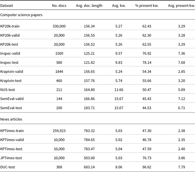
The statistics about the datasets that are used for training and testing of our models are presented in Table 1. Note that there is a big variation in dataset sizes in terms of number of documents (column No. docs), and in an average number of keywords (column Avg. kw.) and present keywords per document (columns Avg. present kw.), ranging from 2.35 present keywords per document in KPTimes-valid to 7.79 in DUC-test.
4.2 Experimental design
We conducted experiments on the datasets described in Section 4.1. First, we lowercased and tokenized all datasets. We experimented with two tokenization schemes, word tokenization and Sentencepiece (Kudo and Richardson Reference Kudo and Richardson2018) byte pair encoding (see Section 6 for more details on how these two tokenization schemes affect the overall performance). During both tokenization schemes, a special $< {eos}> $
token is used to indicate the end of each sentence. For the best-performing model, for which the results are presented in Section 4.4, byte pair encoding was used. For generating the additional POS tag sequence input described in Section 3.1, which was not used in the best-performing model, Averaged Perceptron Tagger from the NLTK library (Bird and Loper Reference Bird and Loper2004) was used. The neural architecture was implemented in PyTorch (Paszke et al. Reference Paszke, Gross, Massa, Lerer, Bradbury, Chanan, Killeen, Lin, Gimelshein, Antiga, Desmaison, Kopf, Yang, DeVito, Raison, Tejani, Chilamkurthy, Steiner, Fang, Bai and Chintala2019).
$< {eos}> $
token is used to indicate the end of each sentence. For the best-performing model, for which the results are presented in Section 4.4, byte pair encoding was used. For generating the additional POS tag sequence input described in Section 3.1, which was not used in the best-performing model, Averaged Perceptron Tagger from the NLTK library (Bird and Loper Reference Bird and Loper2004) was used. The neural architecture was implemented in PyTorch (Paszke et al. Reference Paszke, Gross, Massa, Lerer, Bradbury, Chanan, Killeen, Lin, Gimelshein, Antiga, Desmaison, Kopf, Yang, DeVito, Raison, Tejani, Chilamkurthy, Steiner, Fang, Bai and Chintala2019).
In the pretraining phase, two language models were trained for up to 10 epochs, one on the concatenation of all the texts from the computer science domain and the other on the concatenation of all the texts from the news domain. Overall the language model train set for computer science domain contained around 87 million tokens and the news train set about 232 million tokens. These small sizes of the language model train sets enable relatively fast training and smaller model sizes (in terms of number of parameters) due to the reduced vocabulary.
Table 1. Datasets used for empirical evaluation of keyword extraction algorithms. No.docs stands for number of documents, Avg. doc. length stands for average document length in the corpus (in terms of number of words, that is, we split the text by white space), Avg. kw. stands for average number of keywords per document in the corpus, % present kw. stands for the percentage of keywords that appear in the corpus (i.e., percentage of document’s keywords that appear in the text of the document), and Avg. present kw. stands for the average number of keywords per document that actually appear in the text of the specific document
After the pretraining phase, the trained language models were fine-tuned on each dataset’s validation sets (see Table 1), which were randomly split into 80% of documents used for fine-tuning and 20% of documents used for hyperparameter optimization and test set model selection. The documents containing more than 512 tokens are truncated. Next, the documents are sorted according to the token length and split into batches. The documents in each batch are padded with a special $ <{pad}>$
token to the length of the longest document in the batch. Each model was fine-tuned for a maximum of 10 epochs and after each epoch, the trained model was tested on the documents chosen for hyperparameter optimization and test set model selection. The model that showed the best performance (in terms of F1@10 score) was used for keyword detection on the test set. All combinations of the following hyperparameter values were tested before choosing the best combination, which is written in bold in the list below and on average worked best for all the datasets in both domainsFootnote g:
$ <{pad}>$
token to the length of the longest document in the batch. Each model was fine-tuned for a maximum of 10 epochs and after each epoch, the trained model was tested on the documents chosen for hyperparameter optimization and test set model selection. The model that showed the best performance (in terms of F1@10 score) was used for keyword detection on the test set. All combinations of the following hyperparameter values were tested before choosing the best combination, which is written in bold in the list below and on average worked best for all the datasets in both domainsFootnote g:
-
• Learning rates: 0.00005, 0.0001, 0.0003, 0.0005, 0.001.
-
• Embedding size: 256, 512.
-
• Number of attention heads: 4, 8, 12.
-
• Sequence length: 128, 256, 512.
-
• Number of attention layers: 4, 8, 12.
Note that in our experiments, we use the same splits as in related work (Meng et al. Reference Meng, Yuan, Wang, Brusilovsky, Trischler and He2019; Meng et al. Reference Meng, Zhao, Han, He, Brusilovsky and Chi2017; Gallina et al. Reference Gallina, Boudin and Daille2019) for all datasets with predefined splits (i.e., all datasets with train and validation sets, see Table 1). The exceptions are NUS, DUC and JPTimes datasets with no available predefined validation-test splits. For NUS and DUC, 10-fold cross-validation is used and the model used for keyword detection on the JPTimes-test dataset was fine-tuned on the KPTimes-valid dataset. Another thing to consider is that in the related work by Yuan et al. (Reference Yuan, Wang, Meng, Thaker, Brusilovsky, He and Trischler2020), Meng et al. (Reference Meng, Zhao, Han, He, Brusilovsky and Chi2017), Gallina et al. (Reference Gallina, Boudin and Daille2019), Chen et al. (Reference Chen, Zhang, Wu, Yan and Li2018) and Ye and Wang (Reference Ye and Wang2018), to which we are comparing, large datasets KPTimes-train and KP20k-train with 530,000 documents and 260,000 documents, respectively, are used for the classification model training and these trained models are applied on all test sets from the matching domain. On the other hand, we do not train our classification models on these two large train sets but instead use smaller KPTimes-valid and KP20k-valid datasets for training, since we argue that, due to language model pretraining, fine-tuning the model on a relatively small labeled dataset is sufficient for the model to achieve competitive performance. We do however conduct the language model pretraining on the concatenation of all the texts from the computer science domain and the news domain as explained above, and these two corpora also contain texts from KPTimes-train and KP20k-train datasets.
4.3 Evaluation
To asses the performance of the model, we measure F1@k score, a harmonic mean between Precision@k and Recall@k.
In a ranking task, we are interested in precision at rank k. This means that only the keywords ranked equal to or better than k are considered and the rest are disregarded. Precision is the ratio of the number of correct keywords returned by the system divided by the number of all keywords returned by the system,Footnote h or more formally:
 \[precision = \frac{|correct\ returned\ keywords@k|}{|returned\ keywords|}\]
Recall@k is the ratio of the number of correct keywords returned by the system and ranked equal to or better than k divided by the number of correct ground truth keywords:
 \[recall = \frac{|correct\ returned\ keywords@k|}{|correct\ keywords|}\]
Due to the high variance of a number of ground truth keywords, this type of recall becomes problematic if k is smaller than the number of ground truth keywords, since it becomes impossible for the system to achieve a perfect recall. Similar can happen to precision@k, if the number of keywords in a gold standard is lower than k, and the returned number of keywords is fixed at k. We shall discuss how this affects different keyword detection systems in Section 7.
Finally, we formally define F1@k as a harmonic mean between Precision@k and Recall@k:
 \[ F1@k= 2 * \frac{P@k * R@k} {P@k + R@k} \]
In order to compare the results of our approach to other state-of-the-art approaches, we use the same evaluation methodology as Yuan et al. (Reference Yuan, Wang, Meng, Thaker, Brusilovsky, He and Trischler2020) and Meng et al. (Reference Meng, Yuan, Wang, Brusilovsky, Trischler and He2019), and measure F1@k with k being either 5 or 10. Note that F1@k is calculated as a harmonic mean of macro-averaged precision and recall, meaning that precision and recall scores for each document are averaged and the F1 score is calculated from these averages. Same as in the related work, lowercasing and stemming are performed on both the gold standard and the predicted keywords (keyphrases) during the evaluation and the predicted keyword is considered correct only if the stemmed and lowercased forms of predicted and gold-standard keywords exactly match (i.e., partial matches are considered incorrect). Only keywords that appear in the text of the documents (present keywords)Footnote i were used as a gold standard and the documents containing no present keywords were removed, in order to make the results of the conducted experiments comparable with the reported results from the related work.
As is pointed out in the study by Gallina, Boudin, and Daille (Reference Gallina, Boudin and Daille2020), evaluation and comparison of keyphrase extraction algorithms is not a trivial task, since keyphrase extraction models in different studies are evaluated under different, not directly comparable experimental setups. To make the comparison fair, they recommend the testing of the models on the same datasets, using identical gold-standard keyword sets and employing the same preprocessing techniques and parameter settings. We follow these guidelines strictly, when it comes to the use of identical datasets and gold-standard keyword sets, but somewhat deviate from them when it comes to the employment of identical preprocessing techniques and parameter settings employed for different approaches. Since all unsupervised approaches operate on a set of keyphrase candidates, extracted from the input document, Gallina et al. (Reference Gallina, Boudin and Daille2020) argues that the extraction of these candidates and other parameters should be identical (e.g., they select the sequences of adjacent nouns with one or more preceding adjectives of length up to five words in order to extract keyword candidates) for a fair comparison between algorithms. On the other hand, we are more interested in comparison between keyword extraction approaches instead of algorithms alone and argue that the distinct keyword candidate extraction techniques are inseparable from the overall approach and should arguably be optimized for each distinct algorithm. Therefore, we employ the original preprocessing proposed by the authors for each specific unsupervised approach and apply hyperparameters recommended by the authors. For the supervised approaches, we again employ preprocessing and parameter settings recommended by the authors (e.g., we employ word tokenization proposed by the authors of the systems for CopyRNN and CatSeqD, and employ GPT-specific byte pair tokenizer for GPT-2 and GPT-2 + BiLSTM-CRF approaches).
Instead of reimplementing each specific keyword extraction approach, we report results from the original studies whenever possible, that is, whenever the original results were reported for the same datasets, gold-standard keyword sets, and evaluation criteria, in order to avoid any possible biased decisions (e.g., the choice of hyperparameter settings not clearly defined in the original paper) and reimplementation mistakes. The results of the reimplementation are only reported for evaluation on datasets missing in the original studies and for algorithms with the publicly available code with clear usage instructions. If that is not the case, or if we were not able to obtain the source code from the original authors, the reimplementation was not attempted, since it is in most cases almost impossible to reimplement an algorithm accurately just by following the description in the paper (Repar, Martinc, and Pollak Reference Repar, Martinc and Pollak2019).
4.4 Keyword extraction results and comparison to the state of the art
In Table 2, we present the results achieved by TNT-KID and a number of algorithms from the related work on the datasets presented in Table 1. Note that TfIdf, TextRank, YAKE, RaKUn, Key2Vec, and EmbedRank algorithms are unsupervised and do not require any training. KEA, Maui, GPT-2, GPT-2 + BiLSTM-CRF, and TNT-KID were trained on the different validation set for each of the datasets, and CopyRNN and CatSeqD were trained on the large KP20k-train dataset for keyword detection on computer science domain, and on the KPTimes-train dataset for keyword detection on the news domain, since they require a large train set for competitive performance. For two other CopyRNN variants, CorrRNN and Semi-supervised CopyRNN, we only report results on science datasets published in Chen et al. (Reference Chen, Zhang, Wu, Yan and Li2018) and Ye and Wang (Reference Ye and Wang2018) respectively, since the code for these two systems is not publicly available. The published results for CorrRNN were obtained by training the model on the KP20k-train dataset. On the other hand, Semi-supervised CopyRNN was trained on 40,000 labeled documents from the KP20k-train dataset and 400,000 documents without labels from the same dataset.
Table 2. Empirical evaluation of state-of-the-art keyword extractors. Results marked with * were obtained by our implementation or reimplementation of the algorithm and results without * were reported in the related work

For RaKUn (Škrlj et al. Reference Škrlj, Repar and Pollak2019) and YAKE (Campos et al. Reference Campos, Mangaravite, Pasquali, Jorge, Nunes and Jatowt2020), we report results for default hyperparameter settings, since the authors of RaKUn, as well as YAKE’s authors claim that a single hyperparameter set can offer sufficient performance across multiple datasets. We used the author’s official github implementationsFootnote j in the experiments. For Key2Vec (Mahata et al. Reference Mahata, Kuriakose, Shah and Zimmermann2018), we employ the github implementation of the algorithm Footnote k to generate results for all datasets, since the results in the original study are not comparable due to different set of keywords used (i.e., the keywords are not limited to only the ones that appear in text). Since the published code does not contain a script for the training of domain-specific embeddings trained on multiword candidate phrases, GloVe embeddings (Pennington, Socher, and Manning Reference Pennington, Socher and Manning2014) with the dimension of 50 are used instead. Footnote l The EmbedRank results in the original study (Bennani-Smires et al. Reference Bennani-Smires, Musat, Hossmann, Baeriswyl and Jaggi2018) are also not comparable (again, the keywords in the study are not limited to only the ones that appear in text); therefore, we once again use the official github implementationFootnote m of the approach to generate results for all datasets and employ the recommended Sent2Vec embeddings (Pagliardini et al. Reference Pagliardini, Gupta and Jaggi2018) trained on English Wikipedia with the dimension of 700.
For KEA and Maui, we do not conduct additional testing on corpora for which results are not available in the related work (KPTimes, JPTimes, and DUC corpus) due to bad performance of the algorithms on all the corpora for which results are available. Finally, for TfIdf and TextRank, we report results from the related work where available (Yuan et al. Reference Yuan, Wang, Meng, Thaker, Brusilovsky, He and Trischler2020) and use the implementation of the algorithms from the Python Keyphrase Extraction (PKE) libraryFootnote n to generate unavailable results. Same as for RaKUn and YAKE, default hyperparameters are used.
For KEA, Maui, CopyRNN, and CatSeqD, we report results for the computer science domain published in Yuan et al. (Reference Yuan, Wang, Meng, Thaker, Brusilovsky, He and Trischler2020) and for the news domain we report results for CopyRNN published in Gallina et al. (Reference Gallina, Boudin and Daille2019). The results that were not reported in the related work are results for CatSeqD on KPTimes, JPTimes, and DUC, since this model was originally not tested on these three datasets, and the F1@5 score results for CopyRNN on KPTimes and JPTimes. Again, the author’s official github implementationsFootnote o were used for training and testing of both models. The models were trained and tested on the large KPTimes-train dataset with a help of a script supplied by the authors of the papers. Same hyperparameters that were used for KP20k training in the original papers (Meng et al. Reference Meng, Yuan, Wang, Brusilovsky, Trischler and He2019; Yuan et al. Reference Yuan, Wang, Meng, Thaker, Brusilovsky, He and Trischler2020) were used.
We also report results for the unmodified pretrained GPT-2 (Radford et al. Reference Radford, Wu, Child, Luan, Amodei and Sutskever2019) model with a standard feedforward token classification head, and a pretrained GPT-2 with a BiLSTM-CRF token classification head, as proposed in Sahrawat et al. (Reference Sahrawat, Mahata, Kulkarni, Zhang, Gosangi, Stent, Sharma, Kumar, Shah and Zimmermann2020) and described in Section 3.1.Footnote p Note that a pretrained GPT-2 model with a BiLSTM-CRF token classification head in this experiment does not conduct binary classification, but rather employs the sequence labeling procedure from Sahrawat et al. (Reference Sahrawat, Mahata, Kulkarni, Zhang, Gosangi, Stent, Sharma, Kumar, Shah and Zimmermann2020) described in Section 2, which assigns words in the text sequence into three classes. For the unmodified pretrained GPT-2 (Radford et al. Reference Radford, Wu, Child, Luan, Amodei and Sutskever2019) model and a pretrained GPT-2 with a BiLSTM-CRF token classification head, we apply the same fine-tuning regime as for TNT-KID, that is we fine-tune the models for up to 10 epochs on each dataset’s validation sets (see Table 1), which were randomly split into 80% of documents used for training and 20% of documents used for the test set model selection. The model that showed the best performance on this set of documents (in terms of F1@10 score) was used for keyword detection on the test set. We use the default hyperparameters (i.e., sequence length of 512, embedding size of 768, learning rate of 0.00003, 12 attention heads, and a batch size of 8) for both models and the original GPT-2 tokenization regime.
Overall, supervised neural network approaches drastically outperform all other approaches. Among them, TNT-KID performs the best on four datasets in terms of F1@10. It is outperformed by CatSeqD (on NUS and SemEval) or GPT-2+ BiLSTM-CRF (on JPTImes and DUC) on the other four datasets. CatSeqD also performs competitively on KP20k, Krapivin, and KPTimes datasets, but is outperformed by a large margin on three other datasets by both GPT-2 + BiLSTM-CRF and TNT-KID. To be more specific, in terms of F1@10, TNT-KID outperforms the CatSeqD approach by about 20% points on the Inspec dataset, on the DUC dataset, it outperforms CatSeqD by about 30% points, and on JPTimes it outperforms CatSeqD by about 12% points.
The results of CopyRNN, Semi-supervised CopyRNN, and CorrRNN are in a large majority of cases very consistent with CatSeqD. For example, CopyRNN performs slightly better than CatSeqD on DUC and JPTimes, and slightly worse on the other six datasets. Semi-supervised CopyRNN performs slightly worse than CopyRNN on the majority of datasets for which the results are available according to both criteria. On the other hand, CorrRNN slightly outperforms CopyRNN on two out of the three datasets for which the results are available according to both criteria, but is nevertheless still outperformed by CatSeqD on both of these datasets.
Results of TNT-KID are comparable to the results of GPT-2 + BiLSTM-CRF according to both criteria on a large majority of datasets. The difference is the biggest on the SemEval dataset, where the GPT-2 + BiLSTM-CRF is outperformed by TNT-KID by a margin of about 6% points in terms of F1@10. On the other hand, a GPT-2 model with a standard token classification head does perform less competitively on most datasets but still on average outperforms all non-transformer-based algorithms.
In terms of F1@5, GPT-2 + BiLSTM-CRF outperforms TNT-KID on four datasets (KP20k, Inspec, JPTimes, and DUC) and CatSeqD on three (Krapivin, NUS, and SemEval). Nevertheless, in terms of F1@5, TNT-KID offers consistently competitive performance on all datasets and on average still outperforms both of these algorithms. The performances of GPT-2 + BiLSTM-CRF and TNT-KID are comparable on most datasets, with TNT-KID outperforming GPT-2 + BiLSTM-CRF by a relatively small margin on four out of the eight datasets, and GPT-2 + BiLSTM-CRF outperforming TNT-KID on the other four. On average, the performance of these two algorithms in terms of F1@5 is almost identical, with TNT-KID outperforming GPT-2 + BiLSTM-CRF by a very small margin of 0.3% point.
The difference in performance between TNT-KID and the best-performing sequence-to-sequence generation approach towards keyword extraction, CatSeqD, can be partially explained by the difference in training regimes and the fact that our system was designed to maximize recall (see Section 3). Since our system generally detects more keywords than CatSeqD, it tends to achieve better recall, which offers a better performance when up to 10 keywords need to be predicted. On the other hand, a more conservative system that generally predicts less keywords tends to achieve a better precision, which positively affects the F1 score in a setting where only up to five keywords need to be predicted. This phenomenon will be analyzed in more detail in Section 5, where we also discuss the very low results achieved by CatSeqD on the DUC dataset.
When it comes to two other supervised approaches, KEA and Maui, they perform badly on all datasets they have been tested on and are outperformed by a large margin even by all unsupervised approaches. When we compare just unsupervised approaches, EmbedRank and TextRank achieve much better results than the other approaches according to both measures on the Inspec dataset. This is the dataset with the on average shortest documents. On the other hand, both of these algorithms perform uncompetitively in comparison to other unsupervised approaches on two datasets with much longer documents, KPTimes and JPTimes, where RaKUn and TfIdf are the best unsupervised approaches, respectively. Interestingly, EmbedRank and TextRank also achieve the highest F1@10 score out of all unsupervised keyword detectors on the DUC dataset, which also contains long documents. Perhaps, this could be explained by the average number of present keywords, which is much higher for DUC-test (7.79) than for KPTimes-test (2.4) and JPTimes-test (3.86) datasets.
Overall (see row average), TNT-KID offers the most robust performance on the test datasets and is closely followed by GPT-2 + BiLSTM. CopyRNN and CatSeqD are very close to each other according to both criteria. Out of unsupervised approaches, on average all of them offer surprisingly similar performance. Even though graph-based and statistical approaches toward unsupervised keyword extraction are more popular than embedding-based approaches, the best overall performance in terms of F1@10 is offered by the embeddings-based approach EmbedRank. On the other hand, the other embedding-based method Key2Vec performs the worst out of all unsupervised approaches according to both criteria. According to the F1@10 score, the second ranked YAKE on average works slightly better than the third ranked TextRank and also in general offers more steady performance, since it gives the most consistent results on a variety of different datasets. Similar could be said for RaKUn, the best ranked unsupervised algorithm according to the F1@5 score.
Statistical comparison of classifiers over multiple datasets (according to the achieved F1@10 score) is conducted according to the procedure proposed in Demšar (Reference Demšar2006), that is, with the Friedman test (Friedman Reference Friedman1937), and we were able to reject the null hypothesis, which states that there are no statistically significant differences between the tested keyword extraction approaches. This allowed us to proceed with the post hoc Nemenyi test (Nemenyi Reference Nemenyi1963) to find out which keyword extractors achieve statistically significantly different results. Note that only keyword extraction approaches employed on all the datasets are compared. The results are shown in Figure 3. We can see that the Nemenyi test has detected a significant difference in performance between TNT-KID and unsupervised keyword extractors (Key2Vec, TfIdf, RaKUn, Yake, EmbedRank, and TextRank), but was not strong enough to detect statistically significant differences between the five best supervised approaches.

Figure 3. Critical distance diagram showing the results of the Nemenyi test. Two keyword extraction approaches are statistically significantly different in terms of F1@10 if a difference between their ranks (shown in brackets next to the keyword extraction approach name) is larger than the critical distance (CD). If two approaches are connected with a horizontal line, the test did not detect statistically significant difference between the approaches. For the Nemenyi test $\alpha = 0.05$
was used.
$\alpha = 0.05$
was used.
Examples of the TNT-KID keyword detection are presented in the Appendix.
5. Error analysis
In this section, we first analyze the reasons why transformer-based TNT-KID is capable of outperforming other state-of-the-art neural keyword detectors, which employ a generative model, by a large margin on some of the datasets. Second, we gather some insights into the inner workings of the TNT-KID by a visual analysis of the attention mechanism.
5.1 Comparison between TNT-KID and CatSeqD
As was observed in Section 4.4, transformer-based TNT-KID and GPT-2 + BiLSTM-CRF outperform generative models CatSeqD and CopyRNN by a large margin on the Inspec, JPTimes, and DUC datasets. Here, we try to explain this discrepancy by focusing on the difference in performance between the best transformer-based model, TNT-KID, and the best generative model, CatSeqD. The first hypothesis is connected with the statistical properties of the datasets used for training and testing, or more specifically, with the average number of keywords per document for each dataset. Note that CatSeqD is trained on the KP20k-train, when employed on the computer science domain, and on the KPTimes-train dataset, when employed on news. Table 1 shows that both of these datasets do not contain many present keywords per document (KP20k-train 3.28 and KPTimes-train 2.38), therefore, training the model on these datasets conditions it to be conservative in its predictions and to assign less keywords to each document than a more liberal TNT-KID. This gives the TNT-KID a competitive advantage on the datasets with more present keywords per document.
Figure 4(a) shows a correlation between the average number of present keywords per document for each dataset and the difference in performance in terms of F1@10, measured as a difference between an F1@10 score achieved by TNT-KID and an F1@10 score achieved by CatSeqD. The difference in performance is the biggest for the DUC dataset (about 30% points) that on average has the most keywords per document, 7.79, and second biggest for Inspec, in which an average document has 7.68 present keywords.

Figure 4. (a) Relation between the average number of present keywords per document for each test dataset and the difference in performance ( $F1@10_{\textrm{TNT-KID}} - F1@10_{\textrm{CatSeqD}}$
). (b) Relation between the percentage of keywords that appear in the train set for each test dataset and the difference in performance (
$F1@10_{\textrm{TNT-KID}} - F1@10_{\textrm{CatSeqD}}$
). (b) Relation between the percentage of keywords that appear in the train set for each test dataset and the difference in performance ( $F1@10_{\textrm{TNT-KID}} - F1@10_{\textrm{CatSeqD}}$
).
$F1@10_{\textrm{TNT-KID}} - F1@10_{\textrm{CatSeqD}}$
).
The above hypothesis explains why CatSeqD offers competitive performance on the KP20k-test, Krapivin-test, NUS-test, and KPTimes-test datasets with similar number of keywords per document than its two train sets, but does not explain the competitive performance of CatSeqD on the SemEval-test set that has 6.71 present keywords per document. Even more importantly, it does not explain the large difference in performance between TNT-KID and CatSeqD on the JPTimes-test. This suggests that there is another factor influencing the performance of some keyword detectors.
The second hypothesis suggests that the difference in performance could be explained by the difference in training regimes and the different tactics used for keyword detection by the two systems. While TNT-KID is fine-tuned on each of the datasets, no fine-tuning is conducted for CatSeqD that needs to rely only on the information obtained during training on the large KP20k-train and KPTimes-train datasets. This information seems sufficient when CatSeqD is tested on datasets that contain similar keywords than the train sets. On the other hand, this training regime does not work for datasets that have less overlapping keywords.
Figure 4(b) supports this hypothesis by showing strong correlation between the difference in performance in terms of F1@10 and the percentage of keywords that appear both in the CatSeqD train sets (KP20k-train and KPTimes-train for computer science and news domain, respectively) and the test datasets. DUC and Inspec datasets have the smallest overlap, with only 17% of keywords in DUC appearing in the KPTimes-train and with 48% of keywords in Inspec appearing in the KP20k-train set. On the other hand, Krapivin, NUS, KP20k and KPTimes, the test sets on which CatSeqD performs more competitively, are the datasets with the biggest overlap, reaching up to 95% for KPTimes-test.
Figure 4(b) also explains a relatively bad performance of CatSeqD on the JPTimes corpus (see Table 2) despite the smaller average number of keywords per document. Interestingly, despite the fact that no dataset-specific fine-tuning for TNT-KID is conducted on the JPTimes corpus (since there is no validation set available, fine-tuning is conducted on the KPTimes-valid), TNT-KID manages to outperform CatSeqD on this dataset by about 13% points. This suggests that a smaller keyword overlap between train and test sets has less of an influence on the TNT-KID and could be explained with the fact, that CatSeqD considers keyword extraction as a generation task and tries to generate a correct keyword sequence, while TNT-KID only needs to tag an already existing word sequence, which is an easier problem that perhaps requires less specific information gained during training.
According to the Figure 4(b), the SemEval-test set is again somewhat of an outlier. Despite the keyword overlap that is quite similar to the one in the JPTimes-test set and despite having a relatively large set of present keywords per document, CatSeqD still performs competitively on this corpus. This points to a hypothesis that there might be another unidentified factor, either negatively influencing the performance of TNT-KID and positively influencing the performance of CatSeqD, or the other way around.
5.2 CatSeqD fine-tuning
According to the results in Section 4.4, supervised approaches to the keyword extraction task tend to outperform unsupervised approaches, most likely due to their ability to adapt to the specifics of the syntax, semantics and keyword labeling regime of the specific corpus. On the other hand, the main disadvantage of most supervised approaches is that they require a large dataset with labeled keywords for training, which are scarce at least in some languages. In this paper, we argue that the main advantage of the proposed TNT-KID approach is that due to its language model pretraining, the model only requires a small labeled dataset in order to fine-tune the language model for the keyword classification task. This fine-tuning allows the model to adapt to each dataset and leads to a better performance of TNT-KID in comparison to CatSeqD, for which no fine-tuning was conducted.
Even though no fine-tuning was conducted in the original CatSeqD study (Yuan et al. Reference Yuan, Wang, Meng, Thaker, Brusilovsky, He and Trischler2020), one might hypothesize that the performance of CatSeqD could be further improved if the model would be fine-tuned on each dataset, same as TNT-KID. To test this hypothesis, we take the CatSeqD model trained on KP20k, conduct additional training on the SemEval, Krapivin and Inspec validation sets (i.e., all datasets besides KP20k and KPTimes with a validation set), and test these fine-tuned models on the corresponding test sets. Fine-tuning was conducted for up to 100,000 train stepsFootnote q and the results are shown in Figure 5.

Figure 5. Performance of the KP20k trained CatSeqD model fine-tuned on SemEval, Krapivin and Inspec validation sets and tested on the corresponding test sets, in correlation with the length of the fine-tuning in terms of number of train steps. Zero train steps means that the model was not fine-tuned.
Only on one of the three datasets, the Inspec-test set, the performance can be improved by additional fine-tuning. Though the improvement on the Inspec-test set of about 10% points (from 33.5% to 44%) in terms of F1@10 is quite substantial, the model still performs worse than TNT-KID, which achieves F1@10 of 53.6%. The improvement is most likely connected with the fact that the Inspec-test set contains more keywords that do not appear in the KP20k than SemEval and Krapivin-test sets (see Figure 4(b)). Inspec-test set also contains more keywords per document than the other two test sets (7.68 present keywords on average, in comparison to 6.71 present keywords per document in the SemEval-test set and 3.2 in the Krapivin-test set). Since the KP20k train set on average contains only 3.29 present keywords per document, the fine-tuning on the Inspec dataset most likely also adapts the classifier to a more liberal keyword labeling regime.
On the other hand, fine-tuning does not improve the performance on the Krapivin and SemEval datasets. While there is no difference between the fine-tuned and original model on the Krapivin-test set, fine-tuning negatively affects the performance of the model on the SemEval dataset. The F1@10 score drops from about 35% to about 30% after 20,000 train steps. Further fine-tuning does not have any effect on the performance. The hypothesis is that this drop in performance is somewhat correlated with the size of the SemEval validation set, which is much smaller (it contains only 144 documents) than Inspec and Krapivin validation sets (containing 1500 and 1844 documents, respectively), and this causes the model to overfit. Further tests would, however, need to be conducted to confirm or deny this hypothesis.
Overall, 20,000 train steps seem to be enough for model adaptation in each case, since the results show that additional fine-tuning does not have any influence on the performance.
5.3 Dissecting the attention space
One of the advantages of the transformer architecture is its employment of the attention mechanism, that can be analyzed and visualized, offering valuable insights into inner workings of the system and enabling interpretation of how the neural net tackles the keyword identification task. The TNT-KID attention mechanism consists of multiple attention heads (Vaswani et al. Reference Vaswani, Shazeer, Parmar, Uszkoreit, Jones, Gomez, Kaiser and Polosukhin2017)—square matrices linking pairs of tokens within a given text—and we explored how this (activated) weight space can be further inspected via visualization and used for interpretation.
While square attention matrices show importance of the correlations between all tokens in the document for a keyword identification task, we focused only on the diagonals of the matrices, which indicate how much attention the model pays to the “correlation” a specific word has with itself, that is, how important is a specific word for the classification of a specific token as either being a keyword or not. We extracted these diagonal attention scores for eight attention heads of the last out of eight encoders, for each of the documents in the SemEval-test and averaged the scores across an entire dataset by summing together scores belonging to the same position in each head and dividing this sum with the number of documents. Figure 6 shows the average attention score of each of the eight attention heads for each token position. While there are differences between heads, a distinct peak at the beginning of the attention graph can be observed for all heads, which means that heads generally pay more attention to the tokens at the beginning of the document. This suggests that the system has learned that tokens appearing at the beginning of the document are more likely to be keywords (Figure 7 shows the actual keyword count for each position in the SemEval corpus) and once again shows the importance of positional information for the task of keyword identification.
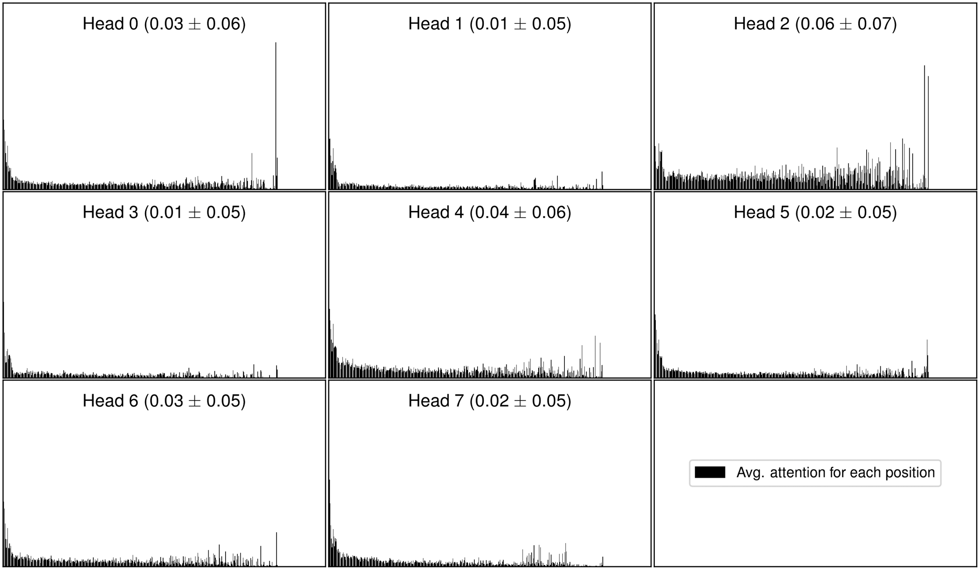
Figure 6. Average attention for each token position in the SemEval corpus across eight attention heads. Distinct peaks can be observed for tokens appearing at the beginning of the document in all eight attention heads.
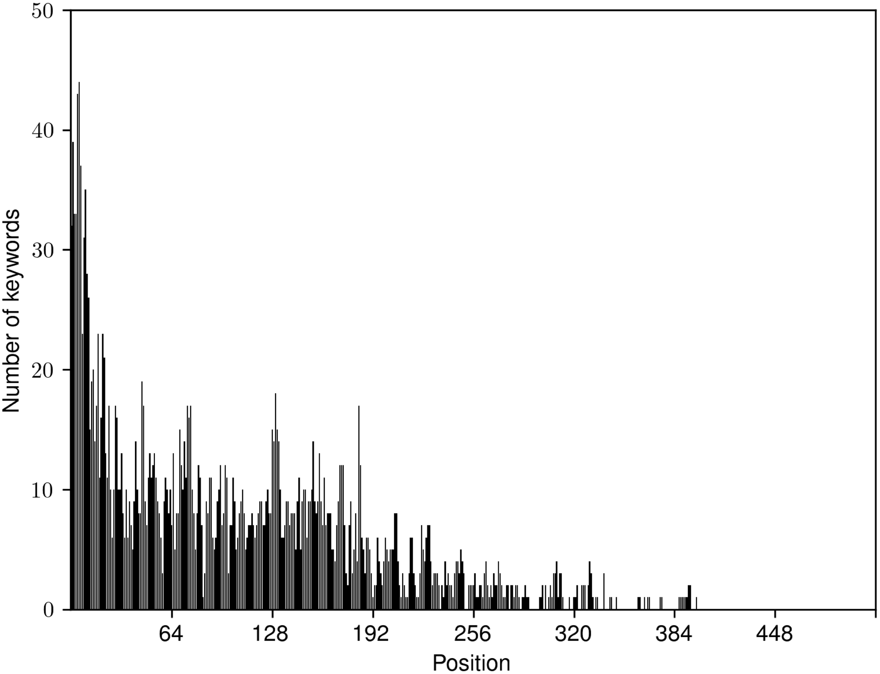
Figure 7. Number of keywords for each token position in the SemEval corpus. Distinct peaks can be observed for positions at the beginning of the document.
Another insight into how the system works can be gained by analyzing how much attention was paid to each individual token in each document. Figure 8 displays attentions for individual tokens, as well as marks them based on predictions for an example document from the SemEval-test. Green tokens were correctly identified as keywords, red tokens were incorrectly identified as keywords, and less transparency (more color) indicates that a specific token received more attention from the classifier.
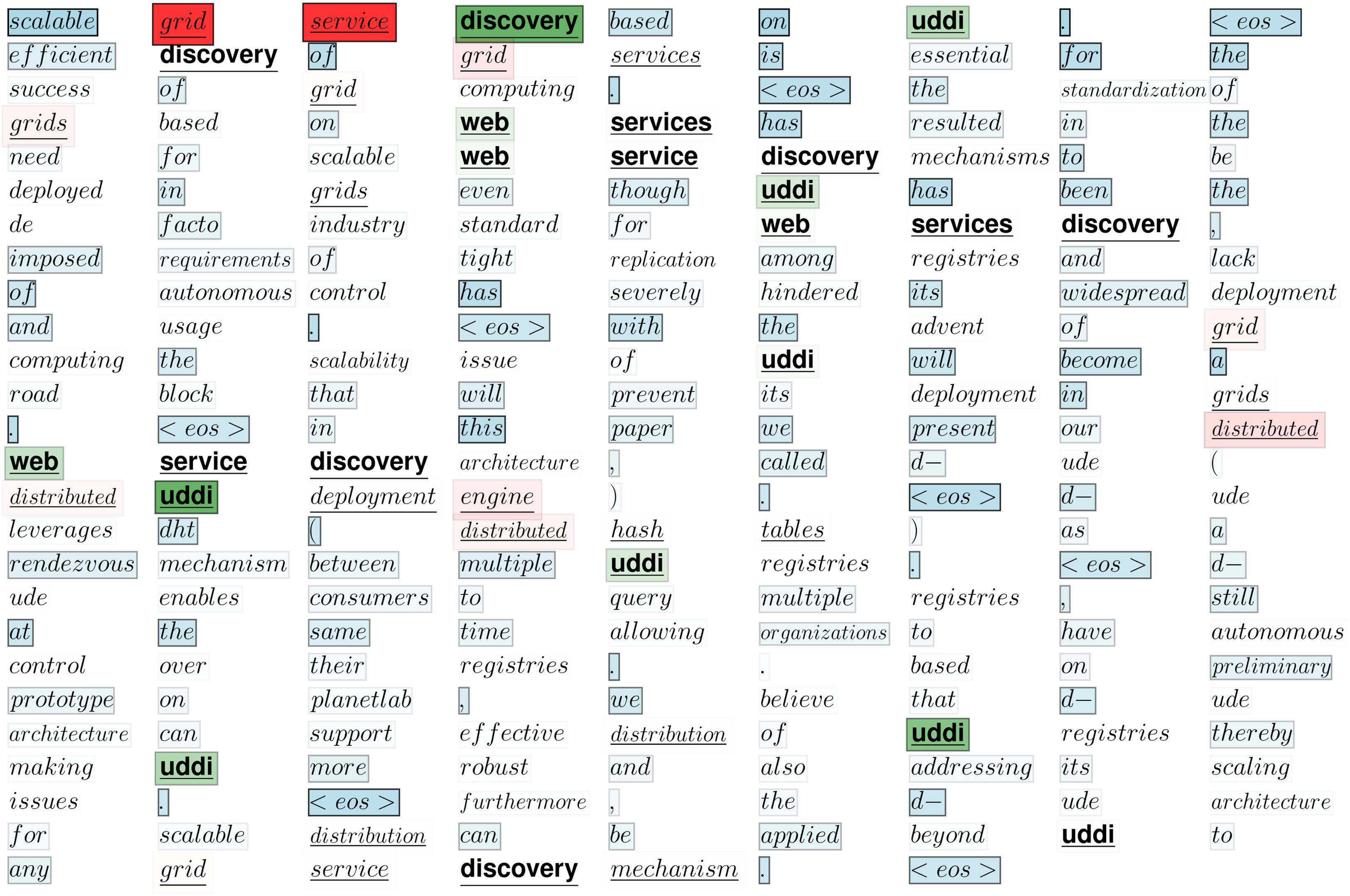
Figure 8. Attention-colored tokens. Underlined phrases were identified as keywords by the system and bold font indicates that the identification was correct (i.e., the keyphrase appears in the gold standard). Less color transparency indicates stronger attention for the token and the color itself designates that the token was correctly identified as keyword (green), incorrectly identified as keyword (red) or was not identified as keyword by the system (blue).
Figure 8 shows that at least for this specific document, many tokens that were either correctly or incorrectly classified as keywords did receive more attention than an average token, especially if they appeared at the beginning of the document. There are also some tokens that received a lot of attention and were not classified as keywords, for example, eos (end of sentence signs) and also words like on, is, has, this, etc. Another interesting thing to notice is the fact that the amount of attention associated with individual tokens that appear more than once in the document varies and is somewhat dependent on the position of the token.Footnote r
6. Ablation study
In this section, we explore the influence of several technique choices and building blocks of the keyword extraction workflow on the overall performance of the model:
• Language model pretraining: assessing whether pretraining positively affects the performance of the keyword extraction and if the improvements are dataset or domain specific.
• Choice of pretraining regime: comparison of two pretraining objectives, autoregressive language modeling and masked language modeling are described in Section 3.2.
• Choice of input tokenization scheme: comparison of two tokenization schemes, word tokenization and Sentencepiece (Kudo and Richardson Reference Kudo and Richardson2018) byte pair encoding.
• Part-of-speech(POS) tags: assessment whether adding POS tags as an additional input improves the performance of the model.
• Transformer architecture adaptations: as was explained in Section 3.1, we propose a re-parametrization of the attention mechanism and in the fine-tuning stage, we add an additional BiLSTM encoder to the output of the transformer encoder. We also experiment with the addition of the BiLSTM+CRF token classification head on top of the model, as was proposed in Sahrawat et al. (Reference Sahrawat, Mahata, Kulkarni, Zhang, Gosangi, Stent, Sharma, Kumar, Shah and Zimmermann2020) and described in Section 3.1. Here we assess the influence of these additions on the performance of the model.
Table 3 presents results on all datasets for several versions of the model, a model with no language model pretraining (noLM), a model pretrained with an autoregressive language model objective (LM), a model pretrained with a masked language model objective (maskedLM), a model pretrained with an autoregressive language model objective and leveraging byte pair encoding tokenization scheme (LM+BPE), a model pretrained with an autoregressive language model objective and leveraging additional POS tag sequence input (LM+POS), a model pretrained with an autoregressive language model objective and a BiLSTM encoder (LM+BiLSTM), a model pretrained with an autoregressive language model objective leveraging byte pair encoding tokenization scheme and a BiLSTM encoder, but without the proposed attention mechanism re-parametrization (LM+BPE+BiLSTM+noAR), a model pretrained with an autoregressive language model objective leveraging byte pair encoding tokenization scheme and a BiLSTM encoder (LM+BPE+BiLSTM), and a model pretrained with an autoregressive language model objective leveraging byte pair encoding tokenization scheme and a BiLSTM+CRF token classification head (LM+BPE+BiLSTM+CRF).
Table 3. Results of the ablation study. Column LM+BPE+BiLSTM represents the results for the model that was used for comparison with other methods from the related work in Section 4.4
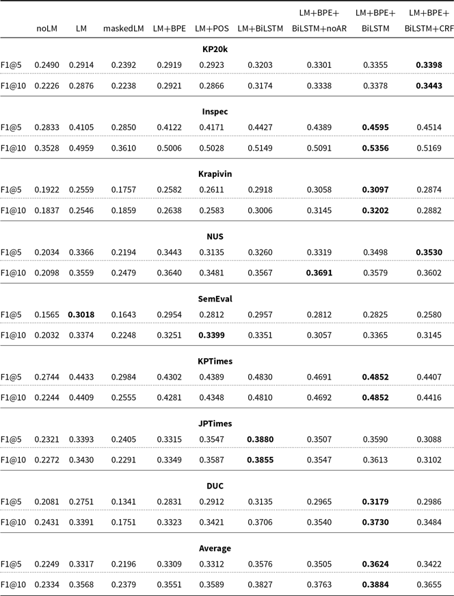
On average (see last two rows in Table 3), by far the biggest boost in performance is gained by employing the autoregressive language model pretraining (column LM), improving the F1@5 score by about 11% points and the F1@10 score by 12% points in comparison to no language model pretraining (column noLM). As expected, the improvements are substantial on two smallest corpora, which by themselves do not contain enough text for the model to obtain sufficient syntactic and semantic knowledge. Large gains are achieved on the NUS test set, where almost an 70% improvement in terms of the F1@10 score can be observed (from 20.98% to 35.59%), and on the SemEval-test set, where the improvement of 93% in terms of F1@5 can be observed. Not surprisingly, for the KP20k dataset, which has a relatively large validation set used for fine-tuning, we can observe a smaller improvement of about 29% in terms of F1@10. On the other hand, we observe the largest improvement of roughly 96% in terms of F1@10 on the KPTimes-test set, even though the KPTimes validation set used for fine-tuning is quite large. This means that in the language modeling phase the model still manages to obtain knowledge that is not reachable in the fine-tuning phase and can perhaps be partially explained by the fact that all documents are truncated into 512 tokens long sequences in the fine-tuning phase. The KPTimes-valid dataset, used both for language modeling and fine-tuning, has on average of 784.65 tokens per document, which means that more than a third of the document’s text is discarded during the fine-tuning phase. This is not the case in the language modeling phase, where all of the text is leveraged.
On the other hand, using the masked language modeling pretraining (column maskedLM) objective on average yields a negligible improvement of about 0.5% points in terms of F1@10 score and worsening of about 0.5% points in terms of F1@10 score in comparison to no language model pretraining. It does, however, improve the performance on the two smallest datasets, NUS (by about 4% points in terms of F1@10) and SemEval (by about 2% points in terms of F1@10). More surprisingly, improvement is also substantial on the KPTimes dataset (about 3% points). The large discrepancy in performance between the two different language model objectives can be partially explained by the sizes of the pretraining corpora. By using autoregressive language modeling, the model learns to predict the next word probability distribution for each sequence in the corpus. By using the masked language modeling objective, 15% of the words in the corpus are randomly masked and used as targets for which the word probability distributions need to be predicted from the surrounding context. Even though each training epoch a different set of words is randomly masked, it is quite possible that some words are never masked due to small sizes of the corpora and since we only train the model for up to 10 epochs.
Results show that adding POS tags as an additional input (column LM+POS) leads to only marginal performance improvements. Some previous studies suggest that transformer-based models that employ transfer learning already capture sufficient amount of syntactic and other information about the composition of the text (Jawahar, Sagot, and Seddah Reference Jawahar, Sagot and Seddah2019). Our results therefore support the hypothesis that additional POS tag inputs are somewhat unnecessary in the transfer learning setting but additional experiments would be needed to determine whether this is task/language specific or not.
Another adaptation that does not lead to any significant improvements when compared to the column LM is the usage of the byte pair encoding scheme (column LM+BPE). The initial hypothesis that motivated the usage of byte pair encoding was that it might help the model’s performance by introducing some knowledge about the word composition and by enabling the model to better understand that different forms of the word can represent the same meaning. However, the usage of byte pair encoding might on the other hand also negatively affect the performance, since splitting up words inside a specific keyphrase would make these keyphrases longer in terms of number of words and detecting a longer continuous word sequence as a keyword might represent a harder problem for the model than detecting a shorter one. Nevertheless, usage of byte pair encoding does have an additional positive effect of drastically reducing the vocabulary of the model (e.g., for news articles, this means a reduction from almost 600,000 tokens to about 32,000) and with it also the number of parameters in the model (from about 630 million to about 80 million).
Adding an additional BiLSTM encoder in the fine-tuning stage of a pretrained model (column LM+BiLSTM) leads to consistent improvements on almost all datasets and to an average improvement of about 3% points in terms of both F1@5 and F1@10 scores. This confirms the findings from the related work that recurrent neural networks work well for the keyword detection task and also explains why a majority of state-of-the-art keyword detection systems leverage recurrent layers.
We also present a model in which we employed autoregressive language model pretraining, used byte pair encoding scheme and added a BiLSTM encoder (column LM+BPE+BiLSTM) that was used for comparison with other methods from the related work in Section 4.4, and the LM+BPE+BiLSTM+noAR model, which employs the same pretraining and tokenization regimes, and also has an added BiLSTM encoder, but was nevertheless not adapted for the keyword extraction task by the re-parametrization of the attention mechanism described in Section 3.1. LM+BPE+BiLSTM outperforms the non-adapted model by a small, yet consistent margin on all but one dataset (on NUS LM+BPE+BiLSTM+noAR performs better in terms of F1@10) according to both criteria.
Finally, we also evaluate the tactic proposed by Sahrawat et al. (Reference Sahrawat, Mahata, Kulkarni, Zhang, Gosangi, Stent, Sharma, Kumar, Shah and Zimmermann2020), where a BiLSTM+CRF token classification head is added on top of the transformer encoder, which employs the byte pair encoding scheme and autoregressive language model pretraining (column LM+BPE+BiLSTM+CRF). The BiLSTM+CRF performs quite well, outperforming all other configurations on two (i.e., on KP20k according to both measures and on NUS accroding to F1@5) datasets. On average, it, however, still performs by more than 2% points worse than LM+BPE+BiLSTM according to both measures. These results suggests that an additional CRF layer is not worth adding to the model when a binary sequence labeling regime is employed, but may nevertheless be useful when classification into more classes needs to be conducted, such as in the case of the labeling regime proposed by Sahrawat et al. (Reference Sahrawat, Mahata, Kulkarni, Zhang, Gosangi, Stent, Sharma, Kumar, Shah and Zimmermann2020) described in Section 2.
7. Conclusion and future work
In this research we have presented TNT-KID, a novel transformer-based neural tagger for keyword identification that leverages a transfer learning approach to enable robust keyword identification on a number of datasets. The presented results show that the proposed model offers a robust performance across a variety of datasets with manually labeled keywords from two different domains. By exploring the differences in performance between our model and the best-performing generative model from the related work, CatSeqD by Yuan et al. (Reference Yuan, Wang, Meng, Thaker, Brusilovsky, He and Trischler2020), we manage to pinpoint strengths and weaknesses of each keyword detection tactic (i.e., keyword labeling and keyword generation) and therefore enable a potential user to choose the approach most suitable for the task at hand. By visualizing the attention mechanism of the model, we try to interpret classification decisions of the neural network and show that efficient modeling of positional information is essential in the keyword detection task. Finally, we propose an ablation study which shows how specific components of the keyword extraction workflow influence the overall performance of the model.
The biggest advantage of supervised approaches to keyword extraction task is their ability to adapt to the specifics of the syntax, semantics, content, genre, and keyword tagging regime of the specific corpus. Our results show that this offers a significant performance boost and state-of-the-art supervised approaches outperform state-of-the-art unsupervised approaches on the majority of datasets. On the other hand, the ability of the supervised models to adapt might become limited in cases when the train dataset is not sufficiently similar to the dataset on which keyword detection needs to be performed. This can clearly be seen on the DUC dataset, in which only about 17% of keywords also appear in the KPTimes train set, used for training the generative CopyRNN and CatSeqD models. Here, these two state-of-the-art models perform the worst of all the models tested and as is shown in Section 5.2, this keywordinees generalization problem cannot be overcome by simply fine-tuning these state-of-the-art systems on each specific dataset.
On the other hand, TNT-KID bypasses the generalization problem by allowing fine-tuning on very small datasets. Nevertheless, the results on the JPTimes corpus suggest that it also generalizes better than CopyRNN and CatSeqD. Even though all three algorithms are trained on the KPTimes dataset (since JPTimes corpus does not have a validation set),Footnote s TNT-KID manages to outperform the other two by about 10% points according to the F1@10 and F1@5 criteria despite the discrepancy between train and test set keywords. As already mentioned in Section 5.1, this can be partially explained by the difference in approaches used by the models and the fact that keyword generation is a much harder task than keyword tagging. For keyword generation task to be successful, seeing a sequence that needs to be generated in advance, during training, is perhaps more important, than for a much simpler task of keyword tagging, where a model only needs to decide if a word is a keyword or not. Even though the keyword generators try to ease the task by employing a copying mechanism (Gu et al. Reference Gu, Lu, Li and Li2016), the experiments suggest that generalizing keywordinees to unseen word sequences still represent a bigger challenge for these models than for TNT-KID.
While the conducted experiments suggest that TNT-KID works better than other neural networks in a setting where previously unseen keywords (i.e., keywords not present in the training set) need to be detected, further experiments need to be devised to evaluate the competitiveness of TNT-KID in a cross-domain setting when compared to unsupervised approaches. Therefore, in order to determine if the model’s internal representation of keywordiness is general enough to be transferable across different domains, in the future we also plan to conduct some cross-domain experiments.
Another aspect worth mentioning is the evaluation regime and how it affects the comparison between the models. By fine-tuning the model on each dataset, the TNT-KID model learns the optimal number of keywords to predict for each specific dataset. This number is in general slightly above the average number of present keywords in the dataset, since the loss function was adapted to maximize recall (see Section 3). On the other hand, CatSeqD and CopyRNN are only trained on the KP20k-train and KPTimes-train datasets that have less present keywords than a majority of test datasets. This means our system on average predicts more keywords per document than these two systems, which negatively affects the precision of the proposed system in comparison to CatSeqD and CopyRNN, especially at smaller k values. On the other hand, predicting less keywords hurts recall, especially on datasets where documents have on average more keywords. As already mentioned in Section 6, this explains why our model compares better to other systems in terms of F1@10 than in terms of F1@5 and also raises a question how biased these measures of performance actually are. Therefore, in the future, we plan to use other performance measures to compare our model to others.
Overall, the differences in training and prediction regimes between TNT-KID and other neural models imply that the choice of a network is somewhat dependent on the use-case. If a large training dataset of an appropriate genre with manually labeled keywords is available and if the system does not need to predict many keywords, then CatSeqD might be the best choice, even though TNT-KID shows competitive performance on a large majority of datasets. On the other hand, if only a relatively small train set is available and it is preferable to predict a larger number of keywords, then the results of this study suggest that TNT-KID is most likely a better choice.
The conducted study also indicates that the adaptation of the transformer architecture and the training regime for the task at hand can lead to improvements in keyword detection. Both TNT-KID and a pretrained GPT-2 model with a BiLSTM + CRF token classification head manage to outperform the unmodified GPT-2 with a default token classification head by a comfortable margin. Even more, TNT-KID manages to outperform both, the pretrained GPT-2 and the GPT-2 with BiLSTM + CRF, even though it employs only 8 attention layers, 8 attention heads and an embedding size of 512 instead of the standard 12 attention layers, 12 attention heads and an embeddings size of 768, which the pretrained GPT-2 employs. The model on the other hand does employ an additional BiLSTM encoder during the classification phase, which makes it slower than the unmodified GPT-2 but still faster than the GPT-2 with the BiLSTM + CRF token classification head that employs a computationally demanding CRF layer.
The ablation study clearly shows that the employment of transfer learning is by far the biggest contributor to the overall performance of the system. Surprisingly, there is a very noticeable difference between performances of two distinct pretraining regimes, autoregressive language modeling and masked language modeling in the proposed setting with limited textual resources. Perhaps a masked language modeling objective regime could be improved by a more sophisticated masking strategy that would not just randomly mask 15% of the words but would employ a more fine-grained entity-level masking and phrase-level masking, similar as in Zhang et al. (Reference Zhang, Han, Liu, Jiang, Sun and Liu2019). This and other pretraining learning objectives will be explored in the future work.
In the future, we also plan to expand the set of experiments in order to also cover other languages and domains. Since TNT-KID does not require a lot of manually labeled data for fine-tuning and only a relatively small domain-specific corpus for pretraining, the system is already fairly transferable to other languages and domains, even to low resource ones. It is especially useful for languages, for which pretrained transformers such as GPT-2, which also perform quite well on the keyword extraction task, do not yet exist. Deploying the system to a morphologically richer language than English and conducting an ablation study in that setting would also allow us to see, whether byte pair encoding and the additional POS tag sequence input would lead to bigger performance boosts on languages other than English.
Finally, another line of research we plan to investigate is a cross-lingual keyword detection. The idea is to pretrain the model on a multilingual corpus, fine-tune it on one language and then conduct zero-shot cross-lingual testing of the model on the second language. Achieving a satisfactory performance in this setting would make the model transferable even to languages with no manually labeled resources.
Acknowledgments
This paper is supported by European Union’s Horizon 2020 research and innovation program under grant agreement No. 825153, project EMBEDDIA (Cross-Lingual Embeddings for Less-Represented Languages in European News Media). We also acknowledge the project Development of Slovene in a Digital Environment co-financed by the Republic of Slovenia and the European Union under the European Regional Development Fund—the project is being carried out under the Operational Programme for the Implementation of the EU Cohesion Policy in the period 2014–2020. The second author was financed via young research ARRS grant. Finally, the authors acknowledge the financial support from the Slovenian Research Agency for research core funding for the program Knowledge Technologies (No. P2-0103) and the project TermFrame—Terminology and Knowledge Frames across Languages (No. J6-9372).
Financial support
The authors were supported by the European Union’s Horizon 2020 research and innovation program under grant agreement No. 825153 (project EMBEDDIA), project Development of Slovene in a Digital Environment co-financed by the Republic of Slovenia and the European Union under the European Regional Development Fund. The second author was financed via young research ARRS grant. Finally, the authors received the financial support from the Slovenian Research Agency for research core funding for the program Knowledge Technologies (No. P2-0103) and the projects TermFrame (No. J6-9372) and CANDAS (No. J6-2581).
Appendix: Examples of keyword identification
Document 1:
Quantum market games. We propose a quantum-like description of markets and economics. The approach has roots in the recently developed quantum game theory”
Predicted keywords: quantum market games, economics, quantum-like description
True keywords: economics, quantum market games, quantum game theory
Document 2:
Revenue Analysis of a Family of Ranking Rules for Keyword Auctions. Keyword auctions lie at the core of the business models of today’s leading search engines. Advertisers bid for placement alongside search results, and are charged for clicks on their ads. Advertisers are typically ranked according to a score that takes into account their bids and potential click-through rates. We consider a family of ranking rules that contains those typically used to model Yahoo! and Google’s auction designs as special cases. We find that in general neither of these is necessarily revenue-optimal in equilibrium, and that the choice of ranking rule can be guided by considering the correlation between bidders’ values and click-through rates. We propose a simple approach to determine a revenue-optimal ranking rule within our family, taking into account effects on advertiser satisfaction and user experience. We illustrate the approach using Monte Carlo simulations based on distributions fitted to Yahoo! bid and click-through rate data for a high-volume keyword.
Predicted keywords: auction, keyword auctions, keyword, ranking rules, ranking, click through rates, click-through rates, revenue, advertiser, revenue analysis
True keywords: revenue optimal ranking, ranking rule, revenue, advertisement, keyword auction, search engine
Document 3:
Profile-driven instruction-level parallel scheduling with application to super blocks. Code scheduling to exploit instruction-level parallelism (ILP) is a critical problem in compiler optimization research in light of the increased use of long-instruction-word machines. Unfortunately, optimum scheduling is computationally intractable, and one must resort to carefully crafted heuristics in practice. If the scope of application of a scheduling heuristic is limited to basic blocks, considerable performance loss may be incurred at block boundaries. To overcome this obstacle, basic blocks can be coalesced across branches to form larger regions such as super blocks. In the literature, these regions are typically scheduled using algorithms that are either oblivious to profile information (under the assumption that the process of forming the region has fully utilized the profile information), or use the profile information as an addendum to classical scheduling techniques. We believe that even for the simple case of linear code regions such as super blocks, additional performance improvement can be gained by utilizing the profile information in scheduling as well. We propose a general paradigm for converting any profile-insensitive list scheduler to a profile-sensitive scheduler. Our technique is developed via a theoretical analysis of a simplified abstract model of the general problem of profile-driven scheduling over any acyclic code region, yielding a scoring measure for ranking branch instructions.
Predicted keywords: scheduling, profile-driven scheduling, instruction-level parallelism, profile-sensitive scheduler, instruction word machines
True keywords: long-instruction-word machines, scheduling heuristic, compiler optimization, optimum scheduling, abstract model, ranking branch instructions, profile-driven instruction-level parallel scheduling, profile-sensitive scheduler, linear code regions, code scheduling
Document 4:
Forty Years After War, Israel Weighs Remaining Risks. JERUSALEM. It was 1 p.m. on Saturday, 6 October 1973, the day of Yom Kippur, the holiest in the Jewish calendar, and Israel’s military intelligence chief, Maj. Gen. Eli Zeira, had called in the country’s top military journalists for an urgent briefing. He told us that war would break out at sundown, about 6 p.m., said Nachman Shai, who was then the military affairs correspondent for Israel’s public television channel and is now a Labor member of Parliament. Forty minutes later he was handed a note and said, Gentlemen, the war broke out, and he left the room. Moments before that note arrived, according to someone else who was at that meeting, General Zeira had been carefully peeling almonds in a bowl of ice water. The coordinated attack by Egypt and Syria, which were bent on regaining strategic territories and pride lost to Israel in the 1967 war, surprised and traumatized Israel. For months, its leaders misread the signals and wrongly assumed that Israel’s enemies were not ready to attack. Even in those final hours, when the signs were unmistakable that a conflict was imminent, Israel was misled by false intelligence about when it would start. As the country’s military hurriedly called up its reserves and struggled for days to contain, then repel, the joint assault, a sense of doom spread through the country. Many feared a catastrophe. Forty years later, Israel is again marking Yom Kippur, which falls on Saturday, the anniversary of the 1973 war according to the Hebrew calendar. This year the holy day comes in the shadow of new regional tensions and a decision by the United States of America to opt, at least for now, for a diplomatic agreement rather than a military strike against Syria in response to a deadly chemical weapons attack in the Damascus suburbs on August 21. Israeli newspapers and television and radio programs have been filled with recollections of the 1973 war, even as the country’s leaders have insisted that the probability of any new Israeli entanglement remains low and that the population should carry on as normal. For some people here, though, the echoes of the past have stirred latent questions about the reliability of intelligence assessments and the risks of another surprise attack. Any Israeli with a 40-year perspective will have doubts, said Mr. Shai, who was the military’s chief spokesman during the Persian Gulf War of 1991, when Israelis huddled in sealed rooms and donned gas masks, shocked once again as Iraqi Scud missiles slammed into the heart of Tel Aviv. Coming after the euphoria of Israel’s victory in the 1967 war, when 6 days of fighting against the Egyptian, Jordanian and Syrian Armies left Israel in control of the Sinai Peninsula, the West Bank, Gaza, East Jerusalem, and the Golan Heights, the conflicts of 1973, 1991, and later years have scarred the national psyche. But several former security officials and analysts said that while the risks now may be similar to those of past years in some respects, there are also major differences. In 1991, for example, the United States of America responded to the Iraqi attack by hastily redeploying some Patriot antimissile batteries to Israel from Europe, but the batteries failed to intercept a single Iraqi Scud, tracking them instead and following them to the ground with a thud. Since then, Israel, and the United States of America have invested billions of dollars in Israel’s air defenses, with the Arrow, Patriot and Iron Dome systems now honed to intercept short-, medium-, and longer range rockets and missiles. Israelis, conditioned by subsequent conflicts with Hezbollah in Lebanon and Hamas in Gaza and by numerous domestic drills, have become accustomed to the wail of sirens and the idea of rocket attacks. But the country is less prepared for a major chemical attack, even though chemical weapons were used across its northern frontier, in Syria, less than a month ago, which led to a run on gas masks at distribution centers here. In what some people see as a new sign of government complacency at best and downright failure at worst, officials say there are enough protective kits for only 60% of the population, and supplies are dwindling fast. Israeli security assessments rate the probability of any attack on Israel as low, and the chances of a chemical attack as next to zero. In 1973, the failure of intelligence assessments about Egypt and Syria was twofold. They misjudged the countries’ intentions and miscalculated their military capabilities. Our coverage of human intelligence, signals intelligence and other sorts was second to none, said Efraim Halevy, a former chief of Mossad, Israel’s national intelligence agency. We thought we could initially contain any attack or repulse it within a couple of days. We wrongly assessed the capabilities of the Egyptians and the Syrians. In my opinion, that was the crucial failure. Israel is in a different situation today, Mr. Halevy said. The Syrian armed forces are depleted and focused on fighting their domestic battles, he said. The Egyptian Army is busy dealing with its internal turmoil, including a campaign against Islamic militants in Sinai. Hezbollah, the Lebanese militant group, is heavily involved in aiding President Bashar al-Assad of Syria, while the Iranians, Mr. Halevy said, are not likely to want to give Israel a reason to strike them, not as the aggressor but as a victim of an Iranian attack. Israel is also much less likely to suffer such a colossal failure in assessment, Mr. Halevy said. We have plurality in the intelligence community, and people have learned to speak up, he said. The danger of a mistaken concept is still there, because we are human. But it is much more remote than before. Many analysts have attributed the failure of 1973 to arrogance. There was a disregarding of intelligence, said Shlomo Avineri, a political scientist at Hebrew University and a director general of Israel’s Ministry of Foreign Affairs in the mid-1970s. War is a maximization of uncertainties, he said, adding that things never happen the same way twice, and that wars never end the way they are expected to. Like most countries, Israel has been surprised by many events in recent years. The two Palestinian uprisings broke out unexpectedly, as did the Arab Spring and the two revolutions in Egypt. In 1973, logic said that Egypt and Syria would not attack, and for good reasons, said Ephraim Kam, a strategic intelligence expert at the Institute for National Security Studies at Tel Aviv University who served for more than 20 years in military intelligence. But there are always things we do not know. Intelligence is always partial, Mr. Kam said, its gaps filled by logic and assessment. The problem, he said, is that you cannot guarantee that the logic will fit with reality. In his recently published diaries from 1973, Uzi Eilam, a retired general, recalled the sounding of sirens at 2 p.m. on Yom Kippur and his rushing to the war headquarters. Eli Zeira passed me, pale-faced, he wrote, referring to the military intelligence chief, and he said: So it is starting after all. They are putting up planes. A fleeting glance told me that this was no longer the Eli Zeira who was so self-assured.
Predicted keywords: Israel, military, Syria, Egypt
True keywords: Israel, Yom Kippur, Egypt, Syria, military, Arab spring
Document 5:
Abe’s 15-month reversal budget fudges cost of swapping people and butter for concrete and guns. The government of Shinzo Abe has just unveiled its budget for fiscal 2013 starting in April. Abe’s stated intention was to radically reset spending priorities. He is indeed a man of his word. For this is a budget that is truly awesome for its radical step backward into the past a past where every public spending project would do wonders to boost economic growth. It is also a past where a cheaper yen would bring unmitigated benefits to Japan’s exporting industries. None of it is really true anymore. Public works do indeed do wonders in boosting growth when there is nothing there to begin with. But in a mature and well-developed economy like ours, which is already so well equipped with all the necessities of modern life, they can at best have only a one-off effect in creating jobs and demand. And in this globalized day and age, an exporting industry imports almost as much as it exports. No longer do we live in a world where a carmaker makes everything within the borderlines of its nationality. Abe’s radical reset has just as much to do with philosophy as with timelines. Three phrases come to mind as I try to put this budget in a nutshell. They are: from people to concrete, from the regions to the center, and from butter to guns. The previous government led by the Democratic Party of Japan declared that it would put people before concrete. No more building of ever-empty concert halls and useless multiple amenity centers where nothing ever happens. More money would be spent on helping people escape their economic difficulties. They would give more power to the regions so they could decide for themselves what was really good and worked for the local community. Guns would most certainly not take precedence over butter. Or rather over the low-fat butter alternatives popular in these more health-conscious times. All of this has been completely reversed in Abe’s fiscal 2013 budget. Public works spending is scheduled to go up by more than 15% while subsistence payments for people on welfare will be thrashed to the tune of more than 7%. If implemented, this will be the largest cut ever in welfare assistance. The previous government set aside a lump sum to be transferred from the central government’s coffers to regional municipalities to be spent at their own discretion on local projects. This sum will now be clawed back into the central government’s own public works program. The planned increase in spending on guns is admittedly small: a 0.8% increase over the fiscal 2012 initial budget. It is nonetheless the first increase of its kind in 11 years. And given the thrashing being dealt to welfare spending, the shift in emphasis from butter to guns is clearly apparent. One of the Abe government’s boasts is that it will manage to hold down the overall size of the budget in comparison with fiscal 2012. The other one is that it will raise more revenues from taxes rather than borrowing. True enough on the face of it. But one has to remember the very big supplementary budget that the government intends to push through for the remainder of fiscal 2012. The money for that program will come mostly from borrowing. Since the government is talking about a 15-month budget that seamlessly links up the fiscal 2012 supplementary and fiscal 2013 initial budgets, they should talk in the same vein about the size of their spending and the borrowing needed to accommodate the whole 15-month package. It will not do to smother the big reset with a big coverup.
Predicted keywords: Shinzo Abe, Japan, economy
True keywords: Shinzo Abe, budget


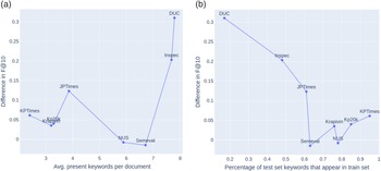


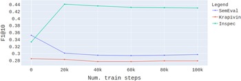
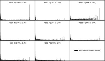

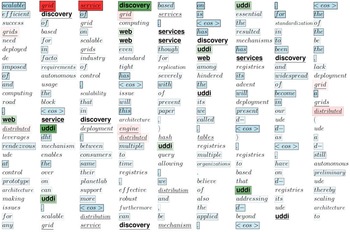


 Open access