


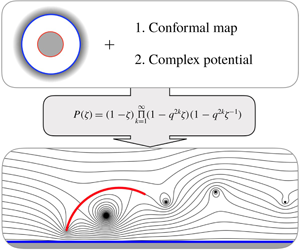
1 Introduction
Understanding ground effect is of intense interest to researchers seeking to comprehend natural flight (Rayner Reference Rayner1991) and design efficient vehicles (Rozhdestvensky Reference Rozhdestvensky2006). The performance improvements due to ground effect are well documented, and include enhancements in the lift-to-drag ratio (Ahmed and Goonaratne Reference Ahmed and Goonaratne2002) and propulsive efficiency (Quinn et al. Reference Quinn, Moored, Dewey and Smits2014). Despite the appeal of understanding ground effect, associated analytic studies have been limited; some progress has been made through vortex models (Coulliette and Plotkin Reference Coulliette and Plotkin1996) and asymptotic analyses in regimes such as extreme ground effect (Widnall and Barrows Reference Widnall and Barrows1970; Tuck Reference Tuck1980), weak ground effect (Iosilevskii Reference Iosilevskii2008), and linearised thin aerofoils (Katz and Plotkin Reference Katz and Plotkin2001; Tomotika, Nagamiya & Takenouti Reference Tomotika, Nagamiya and Takenouti1933), but a uniformly valid theory is still lacking. In particular, there are no analytic studies of moderate ground effect, despite experimental data indicating that this regime exhibits unique physical behaviour, such as flow-mediated equilibria (Kurt et al. Reference Kurt, Cochran-Carney, Zhong, Mivehchi, Quinn and Moored2019). Moreover, previous analytic works have only considered simple physical flow phenomena, such as background uniform flows, linearised wakes, or small-amplitude motions of the wing.
Perhaps one reason for the lack of analytic studies is the complicated topology associated with ground effect. Since the wing is not in contact with the ground, the flow domain contains an irreducible loop (for example, any closed loop containing the wing) and the domain is therefore doubly connected. Although such domains have historically proved resilient to analytic treatments, recent work (for example, Crowdy and Marshall Reference Crowdy and Marshall2006a; Crowdy Reference Crowdy2010, Reference Crowdy2020) has elucidated the underlying mathematical structure of more general multiply connected domains. In particular, Crowdy (Reference Crowdy2010) demonstrated the relevance of a family of special transcendental functions – known as the ‘Schottky–Klein prime functions’ – for solving fluids problems in multiply connected domains. By adapting the approach of Crowdy (Reference Crowdy2010), we account for the doubly connected topology of ground effect by using a special case of the prime function, thereby allowing exact solutions for the potential flow problem. Accordingly, our theory captures all asymptotic regimes and is not limited to a linearised geometry. Additionally, our solution is fully capable of modelling all potential flow phenomena, such as point vortices to represent a shedding wake.
Our mathematical solution involves two steps. The first step is to determine an appropriate coordinate transformation (i.e. a conformal map) from a doubly connected annulus to the physical domain of interest. We offer several suggestions for such maps, including an analogue of the classical Joukowski map (Joukowski Reference Joukowski1910) for ground effect. The second step in the solution is the construction of the complex potential inside the annular domain, which we perform using the ‘new calculus of vortex dynamics’ by Crowdy (Reference Crowdy2010). We provide closed-form representations of the solution for each step.
The remainder of the paper is arranged as follows. In § 2, we present our mathematical model for ground effect. In § 3, we present the mathematical solution to the model. We begin by presenting analytic expressions for some conformal maps from an annulus to a target physical domain in § 3.1. We then derive solutions for a range of physically relevant flows inside the annulus in § 3.2. In § 4, we compare the potential flow solution to experimental results by interrogating the circulation for a range of distances and angles of attack. Finally, in § 5, we summarise the paper and suggest directions of future research. The code used to produce the theoretical results is available at https://github.com/baddoo/ground-effect, and a video abstract is available at https://youtu.be/LBZZPT6eHsM.

Figure 1. The mathematical model in the present work. A wing is in ground effect in a background flow. The chord length is non-dimensionalised to unity, the angle of attack is  $\unicode[STIX]{x1D6FC}$, and the distance between the leading edge and the ground is $d$. The origin is placed on the ground in-line with the leading edge. A representative pitching motion with the associated von Kármán vortex street is illustrated. The red spirals correspond to vortices with positive circulation, whereas blue spirals denotes vortices with negative circulation.
2 Mathematical model
We consider a two-dimensional, inviscid and incompressible flow with fluid velocity  $\boldsymbol{u}$ in a physical $z$-plane where $z=x+\text{i}y$. We additionally assume that the flow is irrotational except at discrete points where there may be point vortices. Therefore, we may define a complex potential
 $$\begin{eqnarray}\displaystyle w(z)=\unicode[STIX]{x1D719}(z)+\text{i}\unicode[STIX]{x1D713}(z), & & \displaystyle \nonumber\end{eqnarray}$$
 where  $\unicode[STIX]{x1D719}$ and $\unicode[STIX]{x1D713}$ are the velocity potential and streamfunction in the physical $z$-plane, respectively. The complex potential is harmonic, so $\unicode[STIX]{x1D6FB}^{2}w=0$.
We now outline the geometry of our model, which is illustrated in figure 1. We model our flier or swimmer as a wing of non-dimensional length  $1$. The wing is inclined at angle of attack $\unicode[STIX]{x1D6FC}$ and the distance of the leading edge to the ground is $d$. The wing may, in principle, take any shape: by using conformal mappings, our solution is valid for any wing profile. We present closed-form mapping functions for several wing shapes of practical interest in § 3.1. We allow the wing to undergo pitching and heaving motions so that $\unicode[STIX]{x1D6FC}$ and $d$ may depend on time. We also consider a background flow, and may include point vortices in the flow to represent discretised vorticity. The ground and the wing are impermeable, and thus the flow must satisfy a no-flux condition on each of these boundaries. Length and velocity scales have been non-dimensionalised with respect to the chord length and upstream velocity, respectively.
3 Mathematical solution
The doubly connected topology presents a challenge insofar as the mathematical solution is concerned, since most analytic methods are only applicable to simply connected domains. To overcome this difficulty we introduce a special function, expressible as the infinite product
 $$\begin{eqnarray}\displaystyle P(\unicode[STIX]{x1D701})=(1-\unicode[STIX]{x1D701})\mathop{\prod }_{k=1}^{\infty }(1-q^{2k}\unicode[STIX]{x1D701})(1-q^{2k}\unicode[STIX]{x1D701}^{-1}), & & \displaystyle\end{eqnarray}$$
 for  $0<q<1$. We suppress the dependence on $q$ for notational convenience. The function $P(\unicode[STIX]{x1D701})$ is a special case of the aforementioned Schottky–Klein prime function, which is typically used to solve fluid dynamics problems in multiply connected domains (Crowdy Reference Crowdy2010, Reference Crowdy2020). In particular, the significance of the prime function $P(\unicode[STIX]{x1D701})$ is that it is effectively a generalisation of the function $(1-\unicode[STIX]{x1D701})$ to doubly connected domains (Baker Reference Baker1897). A full discussion of this fact is well beyond the scope of the current article, but for now it is sufficient to note that $P(\unicode[STIX]{x1D701})$ is analytic in the annulus $q<|\unicode[STIX]{x1D701}|<q^{-1}$, inside which it never vanishes, except for a simple zero at $\unicode[STIX]{x1D701}=1$. Further details of the prime function $P(\unicode[STIX]{x1D701})$ are provided in § S:1 of the supplementary material that is available online at https://doi.org/10.1017/jfm.2020.149.
Remarkably, both the conformal maps and the complex potentials for a range of flows can be expressed exclusively in terms of the prime function  $P(\unicode[STIX]{x1D701})$.
3.1 Conformal maps
The complicated geometry of the ground effect problem means that it is expedient to construct an analytic solution in a circular domain (labelled  $D_{\unicode[STIX]{x1D701}}$) and then map the solution to the physical domain of interest (labelled $D_{z}$). Without loss of generality, we may define the circular domain to be a concentric annulus bounded by the unit disc. We denote the unit disc as $C_{0}$, whilst the interior circle is denoted by $C_{1}$ and has radius $q$, as illustrated in figure 2. We seek a map, $f$, that relates $C_{0}$ to the ground plane and $C_{1}$ to the wing so that we may write $z=f(\unicode[STIX]{x1D701})$.
We now present four conformal maps of relevance to ground effect. With the exception of the first map (3.2), every map presented herein is novel in its application to ground effect. In the following formulae, the constant  $A$ is used to rotate or rescale the domain, and the constant $s$ is used to shift the domain. The maps are each derived in § S:2 of the supplementary material using the more general results of Crowdy and Marshall (Reference Crowdy and Marshall2006a). The maps are illustrated in figure 2.

Figure 2. The four conformal maps for ground effect. Each map relates an annular domain ( $D_{\unicode[STIX]{x1D701}}$) to the target physical domain ( $D_{z}$). The interior circle $C_{1}$ (red) is mapped to the wing, whereas the unit circle $C_{0}$ (blue) is mapped to the ground plane. Areas outside the domain of definition are shaded in grey.
3.1.1 Circular wing map
The first map is the standard Möbius map
 $$\begin{eqnarray}\displaystyle f(\unicode[STIX]{x1D701})=\frac{1-q^{2}}{4\text{i}q}\times \frac{\unicode[STIX]{x1D701}+1}{\unicode[STIX]{x1D701}-1}+s, & & \displaystyle\end{eqnarray}$$
 which maps  $C_{0}$ to the real axis and $C_{1}$ to a circle of unit diameter centred at $\text{i}(q+q^{-1})/4+(1/2)$.
3.1.2 Flat-plate map
The second map takes the form
 $$\begin{eqnarray}\displaystyle f(\unicode[STIX]{x1D701})=A\frac{P(\unicode[STIX]{x1D701}\text{e}^{2\text{i}\unicode[STIX]{x1D6FC}})}{P(\unicode[STIX]{x1D701})}+s, & & \displaystyle\end{eqnarray}$$
 and maps  $C_{0}$ to the real axis and $C_{1}$ to a flat plate of unit length oriented at angle of attack $\unicode[STIX]{x1D6FC}$. The distance of the plate from the ground is determined by the radius of the interior circle $q$.
$q$.
The map (3.3) was previously used by Crowdy and Marshall (Reference Crowdy and Marshall2006b) to calculate the trajectories of point vortices in multiply connected domains, thereby modelling the transport of oceanic eddies. Furthermore, Crowdy (Reference Crowdy2009) used a similar map to model the spreading phase of the Weis-Fogh lift mechanism for insect flight. However, the map (3.3) has not yet been applied to ground effect. This map is particularly well suited for our problem, as it is a natural generalisation of the famous Joukowski map, which relates the unit disc to a flat-plate aerofoil. Modelling aerofoils as flat plates is ubiquitous in classical (Katz and Plotkin Reference Katz and Plotkin2001) and data-driven (Darakananda et al. Reference Darakananda, da Silva, Colonius and Eldredge2018) aerodynamics, and the inclusion of the ground plane here is a major extension: the plethora of studies using the Joukowski map can now be adapted for ground effect.
In the special case where the plate is parallel to the ground, L’Hôpital’s rule shows that (3.3) degenerates to
 $$\begin{eqnarray}\displaystyle f(\unicode[STIX]{x1D701})=A\unicode[STIX]{x1D701}\frac{P^{\prime }(\unicode[STIX]{x1D701})}{P(\unicode[STIX]{x1D701})}+s. & & \displaystyle\end{eqnarray}$$
Both (3.3) and (3.4) are examples of doubly connected Schwarz–Christoffel mappings that can be derived using the formula of Crowdy (Reference Crowdy2007).
3.1.3 Circular arc wing map
The third map transplants  $C_{0}$ to the real axis and $C_{1}$ to a circular arc with centre located in the upper half-plane. The map takes the functional form
 $$\begin{eqnarray}\displaystyle f(\unicode[STIX]{x1D701})=A\frac{P(\unicode[STIX]{x1D701}\overline{\unicode[STIX]{x1D6FE}})}{P(\unicode[STIX]{x1D701}/\unicode[STIX]{x1D6FE})P(\overline{\unicode[STIX]{x1D6FE}})-P(1/\unicode[STIX]{x1D6FE})P(\unicode[STIX]{x1D701}\overline{\unicode[STIX]{x1D6FE}})}+s & & \displaystyle\end{eqnarray}$$
 for any  $\unicode[STIX]{x1D6FE}\in D_{\unicode[STIX]{x1D701}}$.
3.1.4 Centred circular arc wing map
The fourth map sends  $C_{0}$ to the real axis and $C_{1}$ to a circular arc centred on the real axis. The map may be expressed as
 $$\begin{eqnarray}\displaystyle f(\unicode[STIX]{x1D701})=A\frac{P(\sqrt{\unicode[STIX]{x1D701}}\text{e}^{\text{i}\unicode[STIX]{x1D719}})P(-\sqrt{\unicode[STIX]{x1D701}}\text{e}^{\text{i}\unicode[STIX]{x1D719}})P(q\sqrt{\unicode[STIX]{x1D701}})P(-q\sqrt{\unicode[STIX]{x1D701}})}{P(q\sqrt{\unicode[STIX]{x1D701}}\text{e}^{\text{i}\unicode[STIX]{x1D719}})P(-q\sqrt{\unicode[STIX]{x1D701}}\text{e}^{\text{i}\unicode[STIX]{x1D719}})P(\sqrt{\unicode[STIX]{x1D701}})P(-\sqrt{\unicode[STIX]{x1D701}})}+s & & \displaystyle\end{eqnarray}$$
 for  $\unicode[STIX]{x1D719}\in [0,\unicode[STIX]{x03C0}]$.
The ensuing potential flow solutions are invariant under conformal maps, and are therefore applicable to any geometry. In this paper we only present maps for simple wing shapes, since they admit tractable, closed-form representations; more realistic wing shapes will require numerical conformal mapping procedures.
Finally, it is important to note that each map has a simple pole at  $\unicode[STIX]{x1D701}=1$, i.e.
 $$\begin{eqnarray}\displaystyle f(\unicode[STIX]{x1D701})\sim \frac{a_{\infty }}{\unicode[STIX]{x1D701}-1},\quad \text{as }\unicode[STIX]{x1D701}\rightarrow 1, & & \displaystyle\end{eqnarray}$$
 for constant  $a_{\infty }$ defined for each map in § S:3 of the supplementary material.
3.2 Complex potential
Since we have a conformal map from the annular domain to the physical domain, it is sufficient to calculate the complex potential in the annular domain and then map this solution to the physical domain. We express the complex potential in the  $\unicode[STIX]{x1D701}$-plane as $W(\unicode[STIX]{x1D701})=w(z(\unicode[STIX]{x1D701}))$. To construct $W$ we use the new calculus of vortex dynamics proposed by Crowdy (Reference Crowdy2010), which provides a framework for the calculation of instantaneous complex potentials associated with more general multiply connected domains. We present the instantaneous solutions for five scenarios of interest: circulatory flow, point vortices, uniform flow, straining flow, and unsteady pitching and heaving motions of the wing. In all but the last case, the no-flux condition is equivalent to enforcing that the wing is a streamline, and therefore the complex potential takes constant imaginary part on both $C_{0}$ and $C_{1}$.
We present the solutions here with little explanation; further details may be found in Crowdy (Reference Crowdy2010).
3.2.1 Specifying circulation around the wing:  $W_{\unicode[STIX]{x1D6E4}}(\unicode[STIX]{x1D701})$

We begin with the simplest possible non-trivial flow. Suppose that the flow has no singularities and decays in the far field, but the wing has circulation  $\unicode[STIX]{x1D6E4}$. We may write the corresponding complex potential as
 $$\begin{eqnarray}\displaystyle W_{\unicode[STIX]{x1D6E4}}(\unicode[STIX]{x1D701})=\frac{\unicode[STIX]{x1D6E4}}{2\unicode[STIX]{x03C0}\text{i}}\log (\unicode[STIX]{x1D701}). & & \displaystyle\end{eqnarray}$$
 It is simple to verify that  $W_{\unicode[STIX]{x1D6E4}}$ takes constant imaginary part on $C_{0}$ and $C_{1}$. Furthermore, we may note that the circulation around the ground and the wing must be equal and opposite when there are no singularities in the flow. Later, we will use $W_{\unicode[STIX]{x1D6E4}}$ to set the circulation around the wing to enforce the Kutta condition.
3.2.2 Complex potential for point vortices: $W_{V}(\unicode[STIX]{x1D701})$

Suppose that there is now a point vortex of unit strength embedded in the flow at  $\unicode[STIX]{x1D6FD}$ in the annular domain. Due to Crowdy (Reference Crowdy2010), we know that the corresponding complex potential (subject to a no-flux condition) is given by the Green’s function
 $$\begin{eqnarray}\displaystyle G(\unicode[STIX]{x1D701},\unicode[STIX]{x1D6FD})=\frac{1}{2\unicode[STIX]{x03C0}\text{i}}\log \left(\frac{|\unicode[STIX]{x1D6FD}|P(\unicode[STIX]{x1D701}/\unicode[STIX]{x1D6FD})}{P(\unicode[STIX]{x1D701}\overline{\unicode[STIX]{x1D6FD}})}\right), & & \displaystyle\end{eqnarray}$$
 where the overbar denotes the complex conjugate. Moreover, Crowdy (Reference Crowdy2010) showed that  $G$ produces circulation $-1$ around the object which is the image of $C_{0}$ (the ground) and zero circulation around $C_{1}$ (the wing).
It is worth noting the structure of the Green’s function in (3.9) when compared to the Green’s function for a wing in isolation. In the latter (simply connected) case, the circular domain is the unit disc and the corresponding Green’s function may be constructed by placing an image vortex at the location of the physical vortex reflected in the disc. Conversely, in the doubly connected case (3.9), there is an infinite family of image vortices existing outside the annulus. For a fixed  $\unicode[STIX]{x1D6FD}$, inspection of the infinite product formula (3.1) for the prime function $P(\unicode[STIX]{x1D701})$ shows that the set $\{1/\overline{\unicode[STIX]{x1D6FD}},q^{2k}\unicode[STIX]{x1D6FD},\;\;q^{2k}/\overline{\unicode[STIX]{x1D6FD}}:k\in \mathbb{Z}\setminus \{0\}\}$ represents the full family of image vortices. Accordingly, there are two infinite families of vortices in the physical domain: one located inside the wing and the other located under the ground.
The complex potential for  $N$ vortices located at $\unicode[STIX]{x1D6FD}_{j}\in D_{\unicode[STIX]{x1D701}}$ with strength $\unicode[STIX]{x1D705}_{j}$ may simply be expressed as
 $$\begin{eqnarray}\displaystyle W_{V}(\unicode[STIX]{x1D701})=\mathop{\sum }_{j=1}^{N}\unicode[STIX]{x1D705}_{j}G(\unicode[STIX]{x1D701},\unicode[STIX]{x1D6FD}_{j}). & & \displaystyle\end{eqnarray}$$
An appropriate arrangement of vortices could be used to model the wake shed by the wing through adapting the analysis of Michelin and Llewellyn Smith (Reference Michelin and Llewellyn Smith2009).
3.2.3 Complex potential for uniform flow: $W_{U}(\unicode[STIX]{x1D701})$

We now consider the case where the flow is uniform in the far field. The complex potential for a uniform flow takes the form  $w_{U}\sim z$ as $|z|\rightarrow \infty$ in the physical domain. In the annulus, this condition becomes $W_{U}\sim a_{\infty }/(\unicode[STIX]{x1D701}-1)$ as $\unicode[STIX]{x1D701}\rightarrow 1$. Additionally, the imaginary part of the complex potential must take constant values on $C_{0}$ and $C_{1}$. By slightly adapting Crowdy (Reference Crowdy2010), we may write
 $$\begin{eqnarray}\displaystyle W_{U}(\unicode[STIX]{x1D701})=\unicode[STIX]{x1D701}a_{\infty }\frac{P^{\prime }(\unicode[STIX]{x1D701})}{P(\unicode[STIX]{x1D701})}. & & \displaystyle\end{eqnarray}$$
3.2.4 Complex potential for straining flow: $W_{S}(\unicode[STIX]{x1D701})$

By using a similar approach we may calculate the complex potential for a straining flow. In this case, the complex potential has the asymptotic behaviour  $w_{S}\sim z^{2}/2$ as $|z|\rightarrow \infty$ in the physical plane, in addition to the usual no-flux boundary conditions. The complex potential in the $\unicode[STIX]{x1D701}$-plane is given by
 $$\begin{eqnarray}\displaystyle W_{S}(\unicode[STIX]{x1D701})=\frac{a_{\infty }^{2}}{2}\left(\left(\frac{\unicode[STIX]{x1D701}P^{\prime }(\unicode[STIX]{x1D701})}{P(\unicode[STIX]{x1D701})}\right)^{2}-\frac{\unicode[STIX]{x1D701}P^{\prime }(\unicode[STIX]{x1D701})}{P(\unicode[STIX]{x1D701})}-\frac{\unicode[STIX]{x1D701}^{2}P^{\prime \prime }(\unicode[STIX]{x1D701})}{P(\unicode[STIX]{x1D701})}\right). & & \displaystyle \nonumber\end{eqnarray}$$
 Analogous results for higher-order flows (i.e.  $w\sim z^{n}/n$ as $|z|\rightarrow \infty$) may be derived by taking parametric derivatives of the Green’s function (3.9).
3.2.5 Complex potential for wing motion: $W_{M}(\unicode[STIX]{x1D701})$

We may also consider the case where the wing executes rigid body motions of arbitrary amplitude. We show in § S:4 of the supplementary material that the corresponding instantaneous complex potential evaluated at  $\unicode[STIX]{x1D701}\in C_{1}$ must now satisfy
 $$\begin{eqnarray}\text{Im}[W_{M}(\unicode[STIX]{x1D701})]=\text{Im}\left[-\text{i}{\dot{d}}(t)(f(\unicode[STIX]{x1D701})-\text{i}d(t))+\text{i}\frac{\dot{\unicode[STIX]{x1D6FC}}(t)}{2}|\,f(\unicode[STIX]{x1D701})-\text{i}d(t)|^{2}\right]+I\equiv M(\unicode[STIX]{x1D701},\bar{\unicode[STIX]{x1D701}}),\end{eqnarray}$$
 where the dot corresponds to derivatives with respect to time and  $I$ is a constant defined in (S:4.6). Additionally, the imaginary part of $W_{M}$ should vanish on $C_{0}$. Therefore, $W_{M}$ is an analytic function inside the annulus with prescribed imaginary part on the boundaries given by (3.12). Finding such a function is known as the Schwarz problem, and the solution is given by the Villat formula (Crowdy Reference Crowdy2008). Accordingly, the complex potential may be expressed in terms of the prime function $P(\unicode[STIX]{x1D701})$ as
 $$\begin{eqnarray}\displaystyle W_{M}(\unicode[STIX]{x1D701})=\frac{\unicode[STIX]{x1D701}}{\unicode[STIX]{x03C0}}\oint _{C_{1}}M(\unicode[STIX]{x1D701}_{1},\overline{\unicode[STIX]{x1D701}}_{1})\frac{P^{\prime }(\unicode[STIX]{x1D701}/\unicode[STIX]{x1D701}_{1})}{P(\unicode[STIX]{x1D701}/\unicode[STIX]{x1D701}_{1})}\frac{\text{d}\unicode[STIX]{x1D701}_{1}}{\unicode[STIX]{x1D701}_{1}^{2}}. & & \displaystyle \nonumber\end{eqnarray}$$
3.2.6 Total complex potential
In summary, the total complex potential for a wing in ground effect is simply given by combining the contributions from the various flow phenomena:
 $$\begin{eqnarray}\displaystyle W(\unicode[STIX]{x1D701})=W_{\unicode[STIX]{x1D6E4}}(\unicode[STIX]{x1D701})+W_{V}(\unicode[STIX]{x1D701})+W_{U}(\unicode[STIX]{x1D701})+W_{S}(\unicode[STIX]{x1D701})+W_{M}(\unicode[STIX]{x1D701}). & & \displaystyle \nonumber\end{eqnarray}$$
In its current form, the solution is not unique: thus far we have said nothing about how to fix the circulation around the wing. The Kutta condition is the usual strategy for determining the circulation in aerodynamic applications (Eldredge Reference Eldredge2019). To enforce the Kutta condition, we restrict the velocity at the trailing edge to be finite by setting
 $$\begin{eqnarray}\displaystyle \unicode[STIX]{x1D6E4}=-2\unicode[STIX]{x03C0}\text{i}\unicode[STIX]{x1D701}_{t}\left(\frac{\text{d}W_{V}}{\text{d}\unicode[STIX]{x1D701}}(\unicode[STIX]{x1D701}_{t})+\frac{\text{d}W_{U}}{\text{d}\unicode[STIX]{x1D701}}(\unicode[STIX]{x1D701}_{t})+\frac{\text{d}W_{S}}{\text{d}\unicode[STIX]{x1D701}}(\unicode[STIX]{x1D701}_{t})+\frac{\text{d}W_{M}}{\text{d}\unicode[STIX]{x1D701}}(\unicode[STIX]{x1D701}_{t})\right), & & \displaystyle\end{eqnarray}$$
 where  $\unicode[STIX]{x1D701}_{t}$ is the pre-image of the trailing edge in the $\unicode[STIX]{x1D701}$-plane.
Typical streamlines for each complex potential are presented in figure 3. The case that most exemplifies the ground effect is figure 3(c), which illustrates the uniform flow past a centred circular arc wing with the Kutta condition applied. The highlighted streamline shows that the fluid leaves the trailing edge smoothly, demonstrating that the Kutta condition is satisfied. Only two streamlines appear between the wing and the ground, thus indicating that the flow slows down substantially under the wing. Accordingly, the wing will experience a significant lift force, in this case away from the ground.
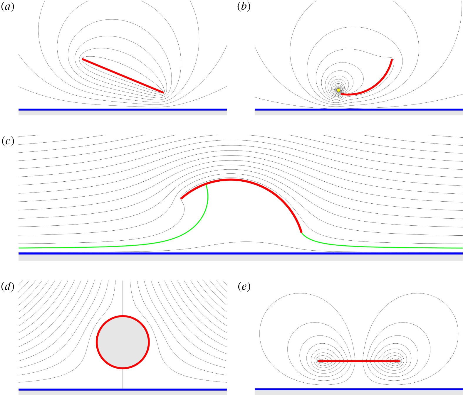
Figure 3. Visualisations of the exact solutions for ground effect for a range of wing shapes. The streamlines are plotted in black, the ground in blue, and the wings in red. The plots show (a) circulatory flow ( $W_{\unicode[STIX]{x1D6E4}}$) around a flat-plate wing at positive angle of attack, (b) a leading-edge vortex ( $W_{V}$) on a circular arc wing, (c) uniform flow ( $W_{U}$) past a centred circular arc wing with the Kutta condition applied at the trailing edge, (d) straining flow ( $W_{S}$) around a circular wing, and (e) instantaneous downward heaving motion ( $W_{M}$) for a flat plate at zero angle of attack. In (b) the yellow dot is the location of the point vortex and in (c) the streamline corresponding to the wing is highlighted in green. The streamlines correspond to linearly spaced values of the streamfunction $\unicode[STIX]{x1D713}$.
4 Experimental validation
In this section we compare our exact ideal solution to experimental data that were collected from flow-visualisation experiments. We consider the case of an inclined flat plate in ground effect embedded in a uniform flow. For the potential flow solution, the relevant conformal mapping is given by (3.3) and the circulation is given by (3.13).
The ground effect experiments were conducted in a closed-loop water channel with a test section of 4.9 m long, 0.93 m wide and 0.61 m deep. The flow was constrained from the bottom and the top with a splitter and surface plate to produce a nominally two-dimensional flow, as shown in figure 4(a). Additionally, a vertical ground plane was installed on the side of the channel. The flat plate used in the experiments has a rectangular planform shape, a 4 % thick cross-section, and a chord and span length of  $c=0.095~\text{m}$ and $s=0.19~\text{m}$
  , respectively. It was constructed from clear acrylic, and polished to be optically transparent for the flow-visualisation. Throughout the experiments, the flow speed, $U$, was kept at $U=0.11~\text{m}~\text{s}^{-1}$, giving a chord-based Reynolds number of $Re=11\,800$. The flat plate was rotated with a servo-motor from its midchord to control the static angle of attack, $\unicode[STIX]{x1D6FC}$. The ground distance $d^{\ast }=d/c$ was changed within the range $0.3\leqslant d^{\ast }\leqslant 3$, and the angle of attack was varied within the range $-3^{\circ }\leqslant \unicode[STIX]{x1D6FC}\leqslant 3^{\circ }$, with $1^{\circ }$ increments for each ground distance.

Figure 4. (a) A schematic of the experimental set-up, (b) vorticity field around the flat plate located at  $d^{\ast }=0.3$ and $\unicode[STIX]{x1D6FC}=1^{\circ }$, (c) the dimensionless circulation and a function of dimensionless ground distance, and (d) normalised circulation as a function of dimensionless ground distance. Square markers are colour indicators for the corresponding $|\unicode[STIX]{x1D6FC}|$ values, both for the experimental data and analytic calculations. (e) Vorticity fields around the flat plate at $\unicode[STIX]{x1D6FC}=-3^{\circ }$ and (f) $\unicode[STIX]{x1D6FC}=3^{\circ }$ located far from the ground at $d^{\ast }=3$, as well as near ground at $d^{\ast }=0.3$ with (g) $\unicode[STIX]{x1D6FC}=-1^{\circ }$, (h) $\unicode[STIX]{x1D6FC}=1^{\circ }$, (i) $\unicode[STIX]{x1D6FC}=-3^{\circ }$, (j) $\unicode[STIX]{x1D6FC}=3^{\circ }$.
Particle image velocimetry (PIV) data were acquired from the flow around the flat plate for each  $(\unicode[STIX]{x1D6FC},d^{\ast })$ case by using an Imager sCMOS camera ( $2560\times 2160$ pixels) and a $200~\text{mJ}~\text{pulse}^{-1}$ Nd:YAG laser (EverGreen 200). The flow was seeded with $11~\unicode[STIX]{x03BC}\text{m}$ hollow metal-coated plastic spherical particles. At the beginning of each run, a digital signal was sent to the programmable timing unit, which triggers both camera and laser at the same time. Each flow field was time-averaged over 100 frames, which were captured at 15 Hz sampling rate. Four passes with two different window sizes were used in the vector calculations, with a final interrogation window size of $48\times 48$ pixels with 75 % overlap. The uncertainty in the instantaneous velocity fields is estimated to be between 1 % and 5 % (Sciacchitano, Wieneke & Scarano Reference Sciacchitano, Wieneke and Scarano2013).
The (clockwise) circulation for each  $(\unicode[STIX]{x1D6FC},d^{\ast })$ case was calculated from the vorticity fields within a rectangular contour by using the area-integral method. The contour was chosen to include the flat plate, but to avoid passing through the boundary layer of the ground wall or the plate, as shown in figure 4(b). For consistency, the selected contour was used for the circulation calculations in all the cases considered here. The small non-zero circulation value obtained for the far-ground case ( $d^{\ast }=3$) at $\unicode[STIX]{x1D6FC}=0^{\circ }$ was subtracted from all other $(\unicode[STIX]{x1D6FC},d^{\ast })$ cases in order to eliminate bias in the system that may be introduced by the presence of the channel walls, small errors in the prescribed angle of attack, or asymmetries in the plate due to manufacturing.
A comparison of the experiments is shown against the present model in figures 4(c) and 4(d). In figure 4(c), the dimensionless clockwise circulation ( $\unicode[STIX]{x1D6E4}^{\ast }=\unicode[STIX]{x1D6E4}/(cU)$) is presented as a function of the dimensionless ground distance and angle of attack. For positive angles of attack (where $\unicode[STIX]{x1D6E4}^{\ast }>0$), the dimensionless circulation is shown to increase as the ground distance decreases and as the angle of attack increases. Here, although experiments at $\unicode[STIX]{x1D6FC}=1^{\circ }$ follow the ideal solution very closely, as $\unicode[STIX]{x1D6FC}$ increases, there is an increasing deviation from the ideal solution. This deviation can be explained by examining the flow fields shown for $\unicode[STIX]{x1D6FC}>0^{\circ }$ far from ground, $d^{\ast }=3$, and near-ground distances, $d^{\ast }=0.3$, presented in figures 4(b), 4(f), and 4(h), 4(j), respectively. In figures 4(b) and 4(h), at $\unicode[STIX]{x1D6FC}=1^{\circ }$, there is no flow separation from the plate either far from or near the ground. However, in figures 4(f) and 4(j), at $\unicode[STIX]{x1D6FC}=3^{\circ }$ the onset of flow separation from the plate is observed, which may lead to a decrease in circulation values from the ideal solution. For the negative angles of attack (where $\unicode[STIX]{x1D6E4}^{\ast }<0$), generally, there is first a mild decrease in the dimensionless circulation (increase in $|\unicode[STIX]{x1D6E4}^{\ast }|$) as the ground distance decreases, in accordance with the ideal solution, and then there is an increase in dimensionless circulation (decrease in $|\unicode[STIX]{x1D6E4}^{\ast }|$) for the closest ground distances. Similarly, the $\unicode[STIX]{x1D6FC}=-1^{\circ }$ cases follow the ideal solution very closely until the closest ground distance, whereas, for $\unicode[STIX]{x1D6FC}=-3^{\circ }$ the deviation from the ideal solution increases as the ground distance decreases. Again, these discrepancies in the experimental data can be explained by examining the flow fields presented for $\unicode[STIX]{x1D6FC}=-3^{\circ }$ at $d^{\ast }=3$, and $\unicode[STIX]{x1D6FC}=-1^{\circ }$ and $-3^{\circ }$ at $d^{\ast }=0.3$, in figures 4(e), 4(g) and 4(i), respectively. Flow separation is observed on the suction side of the plate for $\unicode[STIX]{x1D6FC}=-3^{\circ }$, at $d^{\ast }=3$ in figure 4(e); however, this is found to be suppressed close to the ground at $d^{\ast }=0.3$, as shown in figure 4(i). Additionally, in figures 4(g) and 4(i), there is an interaction between the plate and the ground boundary layer. In both cases, the boundary layer slightly detaches from the ground wall, and elevates towards the shear layers shed from the plate. This elevation is found to increase as $\unicode[STIX]{x1D6FC}$ varies from $-1^{\circ }$ to $-3^{\circ }$, and the detached ground boundary layer is not observed in the $\unicode[STIX]{x1D6FC}>0$ cases. The larger deviations in the experimental data from the ideal solution for $\unicode[STIX]{x1D6FC}<0$ cases can be attributed to these viscous alterations of the flow fields.
Figure 4(d) presents the circulation normalised with the far-from-ground circulation ( $\unicode[STIX]{x1D6E4}_{0}$) for the positive angles of attack, where the model predictions for various angles of attack collapse onto nearly the same curve. Here, the corresponding experimental data follow the same trend as the ideal solutions with 1–15 % deviation. The deviation in the data from the predicted values is higher for the $\unicode[STIX]{x1D6FC}=3^{\circ }$ cases, which may be attributed to flow separation from the plate, which are not accounted for in the ideal solution.
5 Conclusions
We have presented a number of exact solutions for the flow past a wing in ground effect. The solutions are all expressed in terms of the prime function  $P(\unicode[STIX]{x1D701})$ (3.1), which captures the doubly connected topology of the problem. Our solutions extend previous work by permitting more realistic geometries and flow phenomena.
We have also compared our exact, potential flow solution to experimental data in order to identify the missing physics in our model. The data indicate that boundary layer separation is significant, especially in the case of extreme ground effect. These effects are not currently accounted for by our model, although there are several ways that they could be included. The classical remedy is to use asymptotic analysis to solve for the flow in the boundary layers, and then match this to our potential flow solution (Van Dyke Reference Van Dyke1964). Alternatively, a modern approach is to couple our reduced-order potential flow model with a high-fidelity solution via data assimilation (Darakananda et al. Reference Darakananda, da Silva, Colonius and Eldredge2018) to parsimoniously account for boundary layer separation and viscous effects.
The solutions presented in this paper could also be applied to other significant problems in fluid mechanics. For example, we commented earlier that the flat-plate map (3.3) was first used by Crowdy and Marshall (Reference Crowdy and Marshall2006a) to analyse oceanic eddies, and a similar map was exploited by Crowdy (Reference Crowdy2009) to study insect flight. The complex potential solutions presented in § 3.2 are therefore directly applicable to these scenarios, as well as other problems involving an object interacting with a plane wall, such as the vortex shedding by a pipe above a seabed (Price et al. Reference Price, Sumner, Smith, Leong and Païdoussis2002). One way of modelling the complex trajectories of such vortices could be to couple analytic solutions (Crowdy and Marshall Reference Crowdy and Marshall2005) with network-based modelling approaches (Nair and Taira Reference Nair and Taira2015). Finally, the versatility of our solutions are representative of the mathematical techniques deployed in this paper; the Schottky–Klein prime function – of which  $P(\unicode[STIX]{x1D701})$ is just one example – can be used to solve many more problems in multiply connected domains using the methods expounded by Crowdy (Reference Crowdy2010, Reference Crowdy2020).
Acknowledgements
P.J.B. and L.J.A. acknowledge support from EPSRC grants 1625902 and EP/P015980/1, respectively. P.J.B. would like to acknowledge useful conversations with Professor D. Crowdy and Dr R. Nelson at Imperial College London. For the experimental validation part, M.K. and K.W.M. would like to acknowledge the support by the Office of Naval Research under Programme Director Dr R. Brizzolara on MURI grant no. N00014-08-1-0642, as well as by the National Science Foundation under Programme Director Dr R. Joslin in Fluid Dynamics within CBET on NSF CAREER award no. 1653181 and NSF collaboration award no. 1921809.
Declaration of interests
The authors report no conflict of interest.
Supplementary material
Supplementary material is available at https://doi.org/10.1017/jfm.2020.149.


 Open access