


1. Introduction and background
Parameterization of fluxes associated with unresolved dynamics has been an issue in modelling the ocean and atmosphere since its numerical inception. (Indeed many fluid simulations rely on some form of closure for the unresolved scales.) In ocean models we can run ‘eddy-permitting’ climate simulations with 1/4 degree resolution, but these still see only the larger-scale end of the spectrum (several times the first baroclinic Rossby deformation radius and less in the polar oceans). We are getting closer to ‘eddy-resolving’ models, but these still have many unresolved processes – convection, internal wave breaking, coastal processes, etc. Thus, the problem remains important for running long-term climate simulations and also for understanding the biological structure of the ocean. The mixing-length argument, which results in a flux proportional to the local gradient, remains the prevalent technique. In some cases, the eddy diffusivity varies significantly (e.g. the approach developed by Mellor & Yamada Reference Mellor and Yamada1974) but the mixing remains local. Layered models or the popular (Gent & McWilliams Reference Gent and McWilliams1990) scheme reduce artificial cross-isopycnal mixing, but still tend to include an eddy diffusivity for the along-isopycnal mixing, along with an artificial tapering at boundaries or in the mixed layer.
Prandtl's mixing-length theory provides a simple representation of eddy fluxes from a turbulent velocity,  $\boldsymbol{u}'$, avecting a passive trace, $b$, by analogy to molecular processes: $\boldsymbol{\mathcal {K}}\overline {\boldsymbol {u}'b'} =-\boldsymbol{\mathcal{K}} \boldsymbol {\nabla } \bar {b}$. Even though it was clear that this (at least with constant or even spatially varying eddy diffusivity $\boldsymbol{\mathcal {K}}$) was inappropriate for a turbulent boundary layer, the idea became firmly entrenched in most atmospheric and oceanic models and in our ways of thinking of eddies. Indeed, Starr, Peixoto & Gaut (Reference Starr, Peixoto and Gaut1970) choose to express his results on local up-gradient momentum transport in the atmosphere in terms of a ‘negative viscosity’ rather than a breakdown of the simple theory. But up-gradient fluxes can be produced in a number of ways. We shall show that such a locally up-gradient flux can occur, even in tracer transport, due to non-locality. Of course, momentum is neither passive nor a scalar, and as Knobloch (Reference Knobloch1977) discusses, the eddy fluxes even of passive vector fields are not simply down-gradient diffusion. Tracers which are interacting with each other can, even when the local flux assumption holds, end up transporting tracer $b_1$ up the gradient of tracer $b_2$ (Flierl & McGillicuddy Reference Flierl and McGillicuddy2002; Prend et al. Reference Prend, Flierl, Smith and Kaminski2021).
Taylor (Reference Taylor1921) showed the value of thinking about the dispersion problem for a statistically homogeneous flow in a Lagrangian framework and the connection between the Lagrangian autocovariance and  $\boldsymbol{\mathcal {K}}$. He showed that, after an initial adjustment, the patch spread as though acted on by a diffusivity
 \begin{equation} K_{mn}=\int_0^\infty {\rm d}t' \overline{u_m'(\boldsymbol{X}(t,\boldsymbol{x}',t'),t)u_n'(\boldsymbol{x}',t')}. \end{equation}
The velocities here are expressed in Eulerian terms but are tied to the Lagrangian view by  $\boldsymbol {X}(t,\boldsymbol {x}',t')$, the position at time $t$ of the parcel of fluid which was at $\boldsymbol {x}'$ at time $t'$
$t'$
 \begin{equation} \frac{\partial}{\partial t} \boldsymbol{X} = \boldsymbol{u}(\boldsymbol{X},t),\quad \boldsymbol{X}(t',\boldsymbol{x}',t')=\boldsymbol{x}'. \end{equation}
Although this formula is often used to infer eddy diffusivities, it is not really appropriate as a parameterization for several reasons. If you want to know the flux of some property, you care about the properties of the parcels arriving at a point, not departing from it. Therefore, the trajectories need to be traced backwards rather than forwards (cf. Davis Reference Davis1987). For a continuous tracer field, the impact of mixing at unresolved small scales may be important; for example, shear dispersion can be large even though the underlying diffusivity is small. Finally, the actual flux is not simply a diffusivity times a local gradient; this the central theme of our paper.
If we consider the time-averaged flux of a tracer  $b$ across a surface, it will depend on the values of $b$ for the parcels passing the surface at different times; these, in turn, are related to where the parcels came from roughly a decorrelation time before. Thus, we should expect the flux will depend on conditions over a not necessarily small neighbourhood of the surface rather than on the local gradient (in effect, an infinitesimally small neighbourhood). One extension of Taylor's approach involves path integrals (e.g. Drummond Reference Drummond1982) in which the contributions of forcing and diffusion are integrated along a trajectory. The net flux depends on the contributions of all possible paths weighted by the probability of taking such a path. (The similarity to Feynman diagrams is not accidental.) The approaches from Davis (Reference Davis1987, Reference Davis1991) likewise begun with trajectories, but not including diffusion, since he was aiming at the movements of floats rather than dissolved substances (or those which can be represented as a continuum).
Certainly, non-locality is not a new idea. Some parameterizations such as convective adjustment or bulk mixed-layer formulations implicitly recognize that mixing is not local: the mean-free path of a plume may be quite comparable to the scale of variation of the averaged density profile. Other parameterizations include a ‘non-local’ term, such as Large, McWilliams & Doney (Reference Large, McWilliams and Doney1994), but the chosen functional form is empirical. In fact, this non-local nature of mixing has a much broader relevance: it is not uncommon for the scales of variation of the mean or the eddy statistics to be not much greater than the eddies themselves. The non-local nature of the fluxes – the fact that they depend on the gradient not just at the point in question but over a broader region – is implicit in, for example, Davis (Reference Davis1987), but does not seem to have been quantified even for simplified flow models.
Our approach is similar, except that it is framed as an Eulerian problem; in this way, it is close to the more rigorous statistical approach of Kraichnan (Reference Kraichnan1987) and Knobloch (Reference Knobloch1977). However, these deal with homogeneous turbulence, and we are interested in methods that apply to systems with inhomogeneous and/or time-dependent means. But Knobloch (Reference Knobloch1977) shows that the corrections for finite decorrelation times indeed give fluxes which are not simply proportional to the gradient (in his case, the divergence of the flux is expressed as a sum of a series of successively higher even powers of the Laplacian applied to b, rather than the integral formulation we shall work with). Hamba (Reference Hamba2022) takes a similar approach but with spatial/temporal averaging and does not discuss the structure of the kernel. Others have also looked at the nature of the kernel but using various approximations and particular definitions of the mean: Liu, Williams & Mani (Reference Liu, Williams and Mani2023) use a moment method to estimate the non-local diffusivity; however, the flows are steady and the mean is defined as an average over one coordinate. Lavacot et al. (Reference Lavacot, Liu, Williams, Morgan and Mani2023) use the macroscopic forcing method from Mani & Park (Reference Mani and Park2021) to study Rayleigh–Taylor instability; this approach is similar to that of Bhamidipati, Souza & Flierl (Reference Bhamidipati, Souza and Flierl2020). In contrast, we use an ensemble average, both for the theory and the computations, so that we need not rely on averaging over any coordinate (although we take advantage of that to reduce the dimensionality of the kernel to a manageable level), and we present a direct way to compute it.
This paper argues that, for an incompressible flow, the eddy flux is a functional of the mean gradients. We examine the functional and methods for computing it (§ 2) and discuss its characteristics in two-dimensional (2-D) turbulence (§ 3). Properties such as the temporal and spatial decorrelation of the velocities are determined by the dynamics rather than prescribed. Then we briefly show that using artificial flow fields from stochastic velocities (C1 in Appendix C), where we have more control over such statistics, or iterated maps (C2 in Appendix C), which conserve the tracer probability distribution function (PDF), gives very similar pictures of the functional. In some limits, the flux is local, depending only on the mean gradient while in others (much of the range) it is non-local. We give some examples where the breakdown of the ‘eddy diffusivity’ is clear. We emphasize that the formalism is generic; while it may be true that isotropic, three-dimensional (3-D) turbulence is quite local, many flows, not just those in geophysical contexts, also have long-lived, fairly coherent features that can make transport significantly non-local. Convective plumes are, of course, a prime example. Likewise, in wall-bounded turbulence, coherent features (e.g. ‘horse-shoe’ vortices) can appear and move quite far from the wall.
Since time/space averages (as used by Hamba Reference Hamba2022) rely on some statistical homogeneity/stationarity, we shall use an ensemble mean; the mean fields and Reynolds fluxes will be an average over some number  $N$ members each with a different realization of the velocities. We will use subscripts for the velocity components and for ensemble member. But to make the equations more readable, the notation will be abbreviated when unambiguous. For example, the instantaneous flux in the realization $J$ in the $i$th direction of scalar $b$ is
 \begin{equation} F_{i,J} = u'_{i,J}b'_{J} \rightarrow u'_ib' \end{equation}
and the mean eddy flux
 \begin{equation} \bar{F}_{i} = \frac{1}{N}u'_{i,J}b'_{J} \rightarrow \overline{u'_ib'}. \end{equation}
The summation convention – indices repeated on one side but not appearing on the other are summed over – is used.
With these shorthands, our equations describing the evolution of each member of the set of realizations becomes
 \begin{equation} \frac{\partial}{\partial t} b +\boldsymbol{\nabla}\boldsymbol{\cdot}(\boldsymbol{u} b) -\kappa\nabla^2 b = s(\boldsymbol{x},t) \end{equation}
with a diffusivity  $\kappa$ acting at very small scales.
The source/sink field  $s$ is added to ensure that the tracer is not uniform in space and/or time; it is assumed to be the same for each ensemble member, The Reynolds average equations
 $$\begin{gather} \frac{\partial}{\partial t} \bar{b} +\boldsymbol{\nabla}\boldsymbol{\cdot}(\bar{\boldsymbol{u}}\bar{b} +\overline{{\boldsymbol{u}'b'}}) -\kappa\nabla^2 \bar{b} = s, \end{gather}$$
 $$\begin{gather}\frac{\partial}{\partial t} b' +\boldsymbol{\nabla}\boldsymbol{\cdot}(\bar{\boldsymbol{u}} b'+\boldsymbol{u}' b'-\overline{{\boldsymbol{u}'b'}}) -\kappa\nabla^2 b' ={-}\boldsymbol{u}'\boldsymbol{\cdot}\boldsymbol{\nabla}\bar{b} \end{gather}$$
are, of course, the standard form, but it is important to remember that (1.7) is actually a set of  $N$ equations with different $\boldsymbol {u}'$ and $b'$, and that they are coupled by the $\overline {{\boldsymbol {u}'b'}}$ term.
Using high-resolution experiments for calculating a representation ( $\overline {{\boldsymbol {u}'b'}}$ as a functional of $\boldsymbol {\nabla }\bar {b}$) should be approached with (1.7) since this equation, unlike (1.6), simply predicts the mean flux given the mean gradients without requiring knowledge of how those came about. That is the real goal of finding the kernel and, if appropriate, in developing a parameterization.
We remind the reader that the diffusivity above, and the ones we calculate here, convolve the probability of fluid with tracer arriving at some point and the probable concentration within that parcel, i.e. rather than the full PDF of the scalar concentration in space and time,  $P(b, x, t)$, we are only looking at its first moment $\bar{b} = \int {\rm d}b\, P$. For a problem such as release of a toxic material, one really wants to know the likelihood of encountering a concentration above some safe level.
Ensemble averaging has the significant advantage that it does not rely on scale separation (so that local space or time averages can be used in estimating fluxes); therefore the formulae below can be used even when that assumption is not applicable. But it may not be a very good representation that one could use as a parameterization. For example, consider using the simulations like the 2-D ones we will do; could these be used to represent fluxes on a coarser grid which resolves the larger structures but not the finer detail? The problem is that in a snapshot of the field, the fluxes will likely depend on the position and shape of the resolved eddies. This can work when there is significant scale separation so that the large-scale structure can be regarded as uniform over the set of, for example, convective plumes. Techniques like large-eddy simulations have been developed to deal with problems where this is not the case, when the fluxes should depend on the current state, not the ensemble average of the coarse-grained flow. Although the approach discussed below can, in some cases, be used for parameterization, our aim is to gain a better understanding of the physics of tracer transport.
2. Eddy fluxes
We follow lines like Knobloch (Reference Knobloch1977), Kraichnan (Reference Kraichnan1987) and Hamba (Reference Hamba2022) using a Green's function or propagator to write a formal solution for  $b'$. Kraichnan (Reference Kraichnan1987) treats the $\boldsymbol {\nabla }\boldsymbol {\cdot }\overline {\boldsymbol {u}'b'}$ as a forcing term; in contrast, Knobloch (Reference Knobloch1977) includes it in the definition of the propagator, making it an operator rather than a function. Hamba (Reference Hamba2022) also incorporates it in the fluctuation equation using a time/space average. The operator formalism makes the derivation somewhat obscure, and the time/space average will not reveal the time dependence seen in the full form or deal with systems where there are no homogeneous dimensions. Instead, we define an $N\times N$ Green's function matrix for our set of $N$ realizations of the velocity field $\boldsymbol {u}'_J(\boldsymbol {x},t),\ J=1\ldots N$.
We will use a short-hand notation for the left side of (1.7)
 \begin{equation} \frac{\partial}{\partial t} b'_J +\boldsymbol{\nabla}\boldsymbol{\cdot}(\bar{\boldsymbol{u}} b'_J+\boldsymbol{u}'_Jb'_J- \overline{\boldsymbol{u}'b'}-\kappa\boldsymbol{\nabla} b'_J)\equiv {\mathcal{D}}_Jb'_J, \end{equation}
so that our fluctuation equation is just
 \begin{equation} {\mathcal{D}}_J b'_J ={-}\boldsymbol{u}'_J\boldsymbol{\cdot}\boldsymbol{\nabla}\bar{b}. \end{equation}
Remember that the  ${\mathcal {D}}_J$ operator contains an ensemble average, so that the $N$ equations are not independent. Equation (2.2) shows that $b'$ and therefore the flux $\overline {{\boldsymbol {u}'b'}}$ will be a linear functional of $\boldsymbol {\nabla }\bar {b}$.
To find this functional, we can use the Green's function matrix defined by
 \begin{equation} {\mathcal{D}}_JG_{JK} = \delta_{JK}\delta(\boldsymbol{x}-\boldsymbol{x}')\delta(t-t'), \end{equation}
which then gives the fluctuations
 \begin{equation} b'_J ={-}\int {\rm d}\kern1pt\boldsymbol{x}'\,{\rm d}t'G_{JK}(\boldsymbol{x},t\,|\,\boldsymbol{x}',t') \boldsymbol{u}'_K\boldsymbol{\cdot}\boldsymbol{\nabla}\bar{b}. \end{equation}
 Unlike Kraichnan (Reference Kraichnan1987), but like Hamba (Reference Hamba2022), we do not treat the average eddy flux as a forcing, since it could have a complicated spatial-temporal structure which is not known (see also Appendix B). Here, it is included in the calculation of  $G_{JK}$ as the computation proceeds. Requiring the simultaneous solution of a whole set of fields is costly, but the required integration time may be relatively short. We have used Julia (Bezanson et al. Reference Bezanson, Edelman, Karpinski and Shah2017; Besard et al. Reference Besard, Churavy, Edelman and De Sutter2019a; Besard, Foket & De Sutter Reference Besard, Foket and De Sutter2019b) with large ensembles running on a GPU for many of our calculations. Initial conditions for $b'$ can be a problem if $\bar {b}$ is changing with time; however, we shall work with stationary or periodic systems and run for a long enough time for the ensemble members to have lost track of initial conditions. To investigate the effects of changing forcing, one could follow the climate change modelling approach, where the source term is held steady for long enough before $t=0$ when it begins to change.
The eddy flux is now easily found
 \begin{equation} \bar{F}_i(\boldsymbol{x},t)\equiv\overline{u'_i b'} ={-}\int {\rm d}\kern1pt\boldsymbol{x}' \,{\rm d}t' \frac{1}{N} u'_{i,J}(\boldsymbol{x},t)\,G_{JK}\, u'_{j,K}(\boldsymbol{x}',t'){\partial'_j}\,\bar{b}(\boldsymbol{x}',t') \end{equation}
(summed over  $J$ and $K$). The notation $\partial '_i$ mark these as derivatives with respect to $\boldsymbol {x}'$ variables. The flux is thus a weighted integral of the mean gradient
 \begin{equation} \left.\begin{array}{c} \displaystyle\overline{u_i'b'} ={-} \int {\rm d}\kern1pt\boldsymbol{x}' \,{\rm d}t' R_{ij}(\boldsymbol{x},t\,|\,\boldsymbol{x}',t'){\partial'_j}\,\bar{b}(\boldsymbol{x}',t'),\\ \displaystyle R_{ij}(\boldsymbol{x},t\,|\,\boldsymbol{x}',t') = \dfrac{1}{N}u'_{i,J}(\boldsymbol{x},t)G_{JK}(\boldsymbol{x},t\,|\,\boldsymbol{x}',t')u'_{j,K}(\boldsymbol{x}',t'). \end{array}\right\} \end{equation}
 Note that  $R_{ij}$ may have antisymmetric terms that have ‘advective-like character’. To see this, split $R_{ij}$ as
 \begin{equation} R_{ij} = S_{ij}+A_{ij}\quad {\rm with}\ A_{ij}(\boldsymbol{x},t\,|\,\boldsymbol{x}',t')= \tfrac{1}{2}[R_{ij}(\boldsymbol{x},t\,|\,\boldsymbol{x}',t')-R_{ji}(\boldsymbol{x}',t\,|\,\boldsymbol{x},t')]. \end{equation}
This part contributes a term
 \begin{equation} -\int {\rm d}\kern1pt\boldsymbol{x}'\,{\rm d}t' A_{ij}(\boldsymbol{x},t\,|\,\boldsymbol{x}',t'){\partial'_j}\,\bar{b}(\boldsymbol{x}',t'), \end{equation}
to the flux; unlike the symmetric part but like advection, it does not alter the integrated spatial variance in the mean  $\int \textrm {d}\kern0.7pt \boldsymbol {x} |\boldsymbol {\nabla }\bar {b}|^2$.
Phrasing the fluxes in terms of a Green's function helps us see the connection of this Eulerian framework to the Taylor (Reference Taylor1921) form: if the coupling between ensemble members can be ignored, then, in the absence of diffusion,
 \begin{equation} \left(\frac{\partial}{\partial t} + \boldsymbol{u}\boldsymbol{\cdot}\boldsymbol{\nabla}\right)\tilde{G}(\boldsymbol{x},t\,|\,\boldsymbol{x}',t')=\delta(\boldsymbol{x}-\boldsymbol{x}')\delta(t-t'), \end{equation}
and  $\tilde {G}(\boldsymbol {x},t\,|\,\boldsymbol {x}',t')$ is just a delta function at the point $\boldsymbol {x}$ where the fluid parcel originally at $\boldsymbol {x}'$ at time $t'$ has arrived after travelling a time $t-t'$. In essence, the flux depends on the probability of particles with different trajectories hitting the point where the fluxes are being computed and their histories along those trajectories.
The diffusivity in Taylor (Reference Taylor1921) appears when we consider the case in which the mean gradient is constant in time and space; the flux is just
 \begin{equation} \bar{F}_i ={-}K_{ij}\partial_j\bar{b},\quad K_{ij}(\boldsymbol{x},t)=\int {\rm d}\kern1pt\boldsymbol{x}' \,{\rm d}t' \overline{u'_i(\boldsymbol{x},t)G(\boldsymbol{x},t\,|\,\boldsymbol{x}',t')u'_j(\boldsymbol{x}',t')}, \end{equation}
where here  $G$ is given by (2.3) and includes coupling between ensemble members as well as the tracer diffusivity $\kappa$. The parameter $\boldsymbol {u}'(\boldsymbol {x},t)$ can be viewed as the Lagrangian velocity of the particle which started at $\boldsymbol {x}',\ t'$ with velocity $\boldsymbol {u}'(\boldsymbol {x}',t')$. For homogeneous and stationary statistics, the integrand is like the Lagrangian velocity autocorrelation but binned by the travel distance over the time $t-t'$. The $\boldsymbol {x}'$ integral gives a generalized Lagrangian auto-covariance
 \begin{equation} K_{ij}=\int^t {\rm d}\tau L(\tau),\quad L(\tau)=\left[\int {\rm d}\kern1pt\boldsymbol{x}' \overline{u'_i(\boldsymbol{x},t)G(\boldsymbol{x},t\,|\,\boldsymbol{x}',t-\tau)u'_j(\boldsymbol{x}',t-\tau)}\right]. \end{equation}
2.1. Propagators
We can use the fact that the kernel has a summation over  $K$ to simplify the computation somewhat, by writing
 \begin{equation} \phi'_{i,J}(\boldsymbol{x},t\,|\,\boldsymbol{x}',t')=G_{JK}(\boldsymbol{x},t\,|\,\boldsymbol{x}',t')u'_{i,K}(\boldsymbol{x}',t'). \end{equation}
If we multiply (2.3) by  $u'_{i,K}(\boldsymbol {x}',t')$ and sum over $K$, we have the $N$ equations (which are still coupled by the mean flux term) to solve
 \begin{equation} {\mathcal{D}}_J \phi'_{i,J}(\boldsymbol{x},t\,|\,\boldsymbol{x}',t') = u'_{i,J}\delta(\boldsymbol{x}-\boldsymbol{x}')\delta(t-t'), \end{equation}
abbreviated as
 \begin{equation} {\mathcal{D}}\phi'_{i}(\boldsymbol{x},t\,|\,\boldsymbol{x}',t') = u'_{i}\delta(\boldsymbol{x}-\boldsymbol{x}')\delta(t-t')\end{equation}
(Hamba's Reference Hamba2022 Green's function). The resulting flux is
 \begin{equation} \overline{u'_ib'} ={-}\int {\rm d}\kern1pt\boldsymbol{x}' \,{\rm d}t' \overline{u'_{i}(\boldsymbol{x},t)\phi'_{j}(\boldsymbol{x},t\,|\,\boldsymbol{x}',t')}\partial'_j\bar{b}(\boldsymbol{x}',t'), \end{equation}
so that the kernel is
 \begin{equation} R_{ij}(\boldsymbol{x},t\,|\,\boldsymbol{x}',t') = \overline{u'_i(\boldsymbol{x},t)\phi'_j(\boldsymbol{x},t\,|\,\boldsymbol{x}'t')}, \end{equation}
and involves only solving for the coupled set of  $N$ equations for $\phi '_{i,J}$ rather than finding an $N\times N$ matrix. Dropping subscripts in the $R_{ij}$ kernel will indicate isotropy; writing it in terms of $\boldsymbol {x} - \boldsymbol {x}'$ or $t - t'$ implies statistical homogeneity/stationarity. Large-scale spatial or slowly varying time limits are denoted by dropping arguments in $R_{ij}$.
The kernel in the flux expression (2.16), together with the expressions ((2.14), (2.16)) provides a practical method for determining the kernel from simulations. We will be exploring the structure of the kernels using some idealized flow fields.
2.2. Homogeneous isotropic flows
The kernel  $R_{ij}$ depends only on the velocity fields, however, in general it has an 8-D space–time structure in addition to the nine index pairs. To explore its characteristics, we will examine 2-D flows with homogeneous, stationary, nearly (because of the square, doubly periodic domain) isotropic statistics. But it is useful to consider, in general, the implications of homogeneity and isotropy. (In two dimensions, the latter is supplemented by a mirror symmetry $y\rightarrow -y$, equivalent to a 3-D rotation by $180^\circ$ around the $x$-axis.)
Then the kernel satisfies
 \begin{equation} R_{ij}(\boldsymbol{x},t\,|\,\boldsymbol{x}',t') = R_{ij}(|\boldsymbol{x}-\boldsymbol{x}'|, t,t'). \end{equation}
However, we shall show that the kernel for the flux can be expressed more simply with just one scalar function. This can be seen by considering a  $\bar {b}(x_1,t)$ depending only on one coordinate. Isotropy tells us that the flux
 \begin{equation} F_i(\boldsymbol{x},t)={-}\int {\rm d}t'\,{\rm d}\kern1pt x_1'\int {\rm d}\kern1pt x_2'\,{\rm d}\kern1pt x_3' R_{i1}(|\boldsymbol{x}-\boldsymbol{x}'|,t,t')\partial_1\bar{b}, \end{equation}
must have  $F_2=F_3=0$; these fluxes are equally likely to be positive or negative. Therefore the integral will satisfy
 \begin{equation} \int {\rm d}\kern1pt x_2'\,{\rm d}\kern1pt x_3'R_{i1}(|\boldsymbol{x}-\boldsymbol{x}'|,t,t') = 0\quad {\rm for}\ i\ne 1\end{equation}
(as demonstrated from the structure of the tensor in Appendix A), and the flux will be
 \begin{equation} F_i(\boldsymbol{x},t)={-}\delta_{i1}\int {\rm d}t'\,{\rm d}\kern1pt\boldsymbol{x}' R_{11}(|\boldsymbol{x}-\boldsymbol{x}'|,t,t')\,\partial_1\bar{b}. \end{equation}
Note that, if the mean is sinusoidal (the natural basis functions for a translationally invariant operator),  $\bar {b}=b_0\cos kx$, then
 \begin{equation} F_1 = \overline{u_1'b'} = b_0\int {\rm d}\kern1pt\boldsymbol{x}' R_{11}(|\boldsymbol{x}-\boldsymbol{x}'|) \sin kx' = b_0\sin kx \int {\rm d}\kern1pt\boldsymbol{x}'' R_{11}(|\boldsymbol{x}''|) \cos kx'', \end{equation}
with  $\boldsymbol {x}''=\boldsymbol {x}'-\boldsymbol {x}$.
Thus the flux, like the gradient, has a  $\sin kx$ structure, so we can represent it as a wavenumber-dependent diffusivity
 \begin{equation} F_1 ={-}K(k)[{-}b_0\sin kx] ={-}K(k)\partial_1\bar{b}, \end{equation}
with
 \begin{equation} K(k)=\int {\rm d}\kern1pt\boldsymbol{x}'' R_{11}(\boldsymbol{x}'') \cos kx''. \end{equation}
 In Appendix A, we use the Fourier transform of  $\bar {b}$ and the convolution theorem to relate the flux to the transforms of the gradient and the kernel. Adding in the fact that the flux for each component is in the direction of its wavenumber vector leads to
 \begin{equation} F_i(\boldsymbol{x},t)={-}\int {\rm d}t'\,{\rm d}\kern1pt\boldsymbol{x}' R(|\boldsymbol{x}-\boldsymbol{x}'|,t,t')\partial_i\bar{b}, \end{equation}
with a scalar kernel function. Stationarity simply makes this kernel  $R(|\boldsymbol {x}-\boldsymbol {x}'|,t-t')$.
3. Structure of the kernel: 2-D turbulence
Our flow field will be homogeneous and isotropic with mirror symmetry, so we can use (2.23) and estimate  $K(k)$ from the simulations. While we could use the propagator with its delta functions to calculate $R$, it is more straightforward to include the $\sin kx$
 \begin{equation} {\mathcal{D}}\tilde\phi= u_1'(\boldsymbol{x},t)\sin kx\ \Rightarrow K(k) = \overline{u_1'(\boldsymbol{x},t) \tilde\phi(\boldsymbol{x},t)}. \end{equation}
We use  $N$ ensemble members (usually 128) to evaluate $\phi$ so that the averaging can be done during the time integration. When the flow is stationary, we can improve the statistics by also time and $y$ averaging (starting after a long enough time so that the initial conditions do not matter).
For the more general problem without the translational symmetry, we can expand the gradient in some complete set of functions, evaluate the flux for each using (2.14) and (2.16), project the result onto the basis functions and use those to build the kernel. Bhamidipati et al. (Reference Bhamidipati, Souza and Flierl2020) used this approach to study the ocean mixed layer. For our homogeneous, translationally invariant statistics, however, the natural basis functions (mathematically, the eigenfunctions of the integral operator with the kernel having these statistical properties) are sinusoids, and they can be treated individually as above.
We can also use an alternative method in this simple case: solve the full equation
 \begin{equation} \frac{\partial}{\partial t} b +\boldsymbol{\nabla}\boldsymbol{\cdot}(\boldsymbol{u}' b - \kappa \boldsymbol{\nabla} b) = \cos kx, \end{equation}
and least-squares fit  $\bar {b}=b_0\cos kx$, thereby determining $b_0$. The argument above indicates that the flux will be
 \begin{equation} \overline{\boldsymbol{u}'b'} = k K(k) b_0\sin kx, \end{equation}
and substituting this into the mean shows that
 \begin{equation} k^2[K(k)+\kappa] b_0 = 1, \end{equation}
with the cosine and sine terms working out correctly. Then
 \begin{equation} K(k) = \frac{1}{k^2 b_0}-\kappa . \end{equation}
Below, we shall show that the two methods agree to within statistical errors.
The linearity and statistical homogeneity allow us to work directly with the Fourier transform of  $b$, denoted by ${\mathcal {F}}(b)$, and of $s(x_1)$. Each component can be treated as above (or see the convolution argument in Appendix A) so that the flux is
 \begin{equation} {\mathcal{F}}(\bar{F}_i) ={-}{\mathcal{F}}(R_{ij}){\mathcal{F}}(\partial_j\,\bar{b}) = \imath k_j {\mathcal{F}}(R_{ij}){\mathcal{F}}(\bar{b})=\imath k_k K(|\boldsymbol{k}|){\mathcal{F}}(\bar{b}), \end{equation}
and its divergence becomes
 \begin{equation} {\mathcal{F}}(\partial_i\,\bar{F}_i) = k_i k_j {\mathcal{F}}(R_{ij}){\mathcal{F}}(\bar{b})= |\boldsymbol{k}|^2 K(|\boldsymbol{k}|) {\mathcal{F}}(\bar{b}). \end{equation}
Putting this in the transformed mean equation gives us (3.5) for each component so that
 \begin{equation} K(|\boldsymbol{k}|) = \frac{{\mathcal{F}}(s)}{|\boldsymbol{k}|^2{\mathcal{F}}(\bar{b})} -\kappa . \end{equation}
Therefore, we can simply run an experiment with a whole set of wavenumbers representing  ${\mathcal {F}}(s)$ – indeed, in discrete transform space, it could have uniform amplitude ${\mathcal {F}}(s)=1$ – and find the transform of the mean, then use that to compute the effective diffusivity $K(k)$ at each wavenumber. The kernel is the inverse transform of that.
However, we also need  $K(0)$, which cannot be found with the approach above. We calculate that by solving
 \begin{equation} b={-}x+b''\ \Rightarrow \frac{\partial}{\partial t} b'' +\boldsymbol{\nabla}\boldsymbol{\cdot} [\boldsymbol{u}'b''- \kappa \boldsymbol{\nabla} b''] = u_1' \end{equation}
in our periodic domain. The mean  $\overline {\boldsymbol {u}'b''}$ is calculated as an ensemble and spatial mean (and is therefore non-divergent). It will be $c_0\hat {\boldsymbol{x}}$ with $c_0$ constant. Since this does not develop a mean $\bar {b}$, we just have $c_0=K(0)$.
3.1. Flow field
We use a 2-D turbulent flow and simplifications which arise when the statistics of  $\bar {b}$, set by the nature of the sources and sinks, are also independent of some coordinates. For the flow field, the vorticity $\zeta$ satisfies
 \begin{equation} \frac{\partial}{\partial t}\zeta+\boldsymbol{u}\boldsymbol{\cdot}\boldsymbol{\nabla}\zeta = {\mathcal{F}} -\nu\nabla^4\zeta-\nu_h\nabla^{{-}4}\zeta \quad {\rm with}\ \zeta=\nabla^2\psi,\ \boldsymbol{u} = \hat{\boldsymbol{z}}\times\boldsymbol{\nabla}\psi. \end{equation}
We use a fairly standard dissipation with a hyperviscosity and a hypoviscosity to take care of the downscale transfer of enstrophy and the upscale flux of energy. Note that, this flow, like large-scale motions in the atmosphere and ocean, can have fairly long-lived coherent vortices; these tend to make the non-locality more significant.
The forcing  ${\mathcal {F}}$ is nearly spatially white noise with a Fourier transform
 \begin{equation} \hat{\mathcal{F}} = f_0\exp(\imath\theta(\boldsymbol{k},t))\quad \text{for}\ |\boldsymbol{k}|^2 \le 2 \times 16^2 \text{ and } |\boldsymbol{k}|^2 \ne 0 . \end{equation}
The initial phase is random in the range  $[0,2{\rm \pi} )$, and $\theta$ of each forcing wavevector evolves independently as
 \begin{equation} {\rm d}\theta = \sqrt{2}\, {\rm d}W_t, \end{equation}
where  $W_t$ denotes a Wiener process. The forcing amplitude $f_0,\ \nu,\ \nu _h$ are chosen so that the default root-mean-square (r.m.s.) velocity is approximately 1. The default parameters are $f_0=300$, $\nu =5\times 10^{-6}$ and $\nu _h=10^{-3}$; however, $f_0$ will be varied to explore the changes as the flow gets stronger or weaker. The domain size is $4{\rm \pi} \times 4{\rm \pi}$ and is doubly periodic. Numerically, we have used pseudospectral advection with $128\times 128$ grid points and Runge–Kutta fourth-order time stepping. (Various results were checked against a resolution of $256\times 256$ with similar kinetic energies; they are not sensitive to the resolution, the advection scheme, or the time-stepping method.)
For the tracer, the explicit diffusion  $\kappa \nabla ^2 b$ has a default $\kappa$ value of
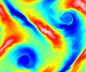
  $10^{-3}$ and plays very little role; the eddy fluxes are generally several orders of magnitude larger. Figure 1 shows an example of the evolution of the full $b$ (1.5) with $s=0$ and the initial condition being a slightly soft-edged circular patch of radius 1 with $b=1$ (panel a). Panel (b) shows one realization at $t=4$; the slight softening of the edges is caused by $\kappa$ and numerical diffusion from filtering to avoid aliasing. When we average many realizations, $\bar {b}$ from an initial patch will, in the mean, spread in a manner resembling eddy diffusion, as we see in panel (c) showing the mean of 5000 realizations (several times more than needed). In this case, with a uniform initial condition $b=1$ within the patch, $\bar {b}(x,t)$ can also be viewed as the probability of seeing $b=1$ at point $\boldsymbol {x}$ and time $t$ (ignoring $\kappa$).

Figure 1. Initial condition, distribution at  $t=4$, and the average at $t=4$ of 5000 realizations of the flow.
In this case, the differences in the spread of the mean from those predicted by a simple eddy diffusion can be found, but are not large. We can illustrate the issues with the diffusion approximation by adding a source term  $s(\boldsymbol {x})$ which, if only local diffusivity were acting, would lead to a fairly sharp-edged circular patch
 \begin{equation} b_0=0.5[1-\tanh(5r-5)]\quad \text{and}\quad s(\boldsymbol{x})={-}\nabla^2 b_0. \end{equation}
If we had a constant  $K_\textit {eff}$ eddy diffusivity, $b$ would be $b_0/(K_\textit {eff}+\kappa )$. However, the mean state is quite different under the advective stirring. Figure 2 shows that sections through the centre have a clear signal of the spikiness in the forcing, evidence of the non-local fluxes. If we consider the point where $\bar {b}$ goes from the positive peak to the negative one, the local approximation would lead to strong fluxes to the right and smooth the peaks away. The kernel (shown later in figure 8), however, is averaging the gradient not just at this point, so it includes the positive $\partial _x\bar {b}$ associated with the neighbouring peak and trough. As a result, we can see that the radial gradient and flux have the same sign near the centre (figure 3) but the more usual opposite signs further out. As a result, the plot of the flux against the gradient (figure 3) is both multivalued and has up-gradient regions with $\boldsymbol {\nabla }\bar {b}$ and $\overline {\boldsymbol {u}'b'}$ the same sign, as well as points where the gradient vanishes but the flux does not. Clearly, representing the flux as a function of the gradient cannot reproduce the structure seen in the experiment.

Figure 2. Cross-sections through the forcing and  $\bar {b}$. The fields are essentially radially symmetric, with a slight asymmetry evident in the $y=0$ vs $x=0$ sections for $\bar {b}$. The forced equation was integrated with 128 ensembles and averaged from $t = 256$ to $t = 4000$ time units. The dotted green line is the solution one would get from an eddy diffusivity.

Figure 3. Cross-sections of the gradient (blue) and flux (red) along the  $x$ and $y$ axes. (a) The curves very nearly overlap for the two different sections. The panel (b) plots the flux vs the gradient with the blue (red) the $x$ (
$x$ ( $\,y$) cut.
3.2. Non-local in space
Our velocity field is homogeneous and stationary, but the tracer can have sources and sinks in different areas, and we expect the flux will be a non-local function of the gradients. To find this, we force with  $s=\cos kx$ for a range of wavenumbers. Then, using either (3.1) or (3.5) gives $K(k)$; the results in figure 4 show that the estimates are the same. The variation of $K(k)$ is clear evidence that the kernel is not local since the flux would then depend only on the local gradient and $K(k)$ would be independent of the mean scale $1/k$.


We note that, even in experiments with  $\kappa =0$ (§ C.2 and arguments in Souza, Lutz & Flierl Reference Souza, Lutz and Flierl2023), $\bar {b}$ settles down with a long enough time average (which indeed can be quite long) or a very large number of ensemble members. Higher moments like $\overline {b'^2}$, however, may not settle. A fluid parcel wandering through the source and sink regions will give a $b'$ which is, in effect, undergoing a random walk and can wander off to large values.
3.3. Large-scale approximation
When the scales of the mean are large in a sense to be determined, we can approximate  $\boldsymbol {\nabla }\bar {b}(\boldsymbol {x}')\simeq \boldsymbol {\nabla }\bar {b}(\boldsymbol {x})$ and remove it from the $\boldsymbol {x}'$ integral in (2.16). (We shall discuss the case with time variation in $\boldsymbol {\nabla }\bar {b}$ below.) Indeed, an oft-used approach is to regard the gradients $\varGamma _j= \partial _j\,\bar {b}$ as strictly constant, in which case, the fluxes are also, and the divergence vanishes. We can then drop the divergence of the mean flux term in ${\mathcal {D}}_J$ and calculate the ensembles separately. As in (2.10), the flux is
 \begin{equation} \bar{F}_i ={-} K_{ij} {\partial_j}\, \bar{b}(\boldsymbol{x}), \end{equation}
which we use to calculate  $K(0)$.
In practice, we use (3.9), which, not surprisingly, agrees with the multi-scale expansion procedure in Papanicolaou & Pironeau (Reference Papanicolaou and Pironeau1981). The effective diffusivity (figure 5) behaves like  $u_0^2\tau$, as expected, but the integral time scale $\tau$ is by no means constant as we increase the forcing strength, $f_0$. Indeed, it decays as roughly $f_0^{-0.7}$ or, in terms of the kinetic energy of the flow, as $E^{-0.4}$.

Figure 5. Value of  $K(0)$ as a function of the kinetic energy (equal to the covariance at zero lag $\overline {u(\boldsymbol {x},0)^2}$). This is the down-gradient eddy diffusivity when the mean gradients are at scales much larger than the eddy scale. The thin red line is the version calculated from the Lagrangian covariance, § 3.5, while the thick orange dashes show the fit $1.7 (\overline {u^2})^{0.52}$.
Appendix B cautions about calculating the fluxes by including the large-scale gradient as part of the forcing; i.e. solving
 \begin{equation} \frac{\partial}{\partial t} b' + \boldsymbol{\nabla}\boldsymbol{\cdot}[(\bar{\boldsymbol{u}}+\boldsymbol{u}')b'-\kappa\boldsymbol{\nabla} b'] = u'(\boldsymbol{x},t) g(\epsilon x), \end{equation}
directly and computing the fluxes and their large-scale divergence. The results, even for small but finite  $\epsilon$, will not agree with a computation
 \begin{equation} {\mathcal{D}} b' = u' (\boldsymbol{x},t) g(\epsilon x), \end{equation}
including the  $\boldsymbol {\nabla }\boldsymbol {\cdot }\overline {\boldsymbol {u}' b '}$ term. Thus the multi-scale approximation must be approached carefully when the scale separation is not terribly large.
If we plot  $K(k)$ vs the scale $1/k$ of $\bar {b}$ divided by the ‘mean-free path’ $\sqrt {E}\,\tau$ (figure 6) we see that it becomes constant when the gradients have a scale of the order of 2–4 times larger. But the mean-free path is often not small in the atmosphere ( $u_0\sim 50$ m s $^{-1}$ with $\tau \sim 3 d \rightarrow 13\,000\ \textrm {km}$) or ocean (0.3 m s $^{-1}$, $30 d\rightarrow 780\ \textrm {km}$); convective plumes likewise span the domain over which the temperature varies. It seems likely that horse-shoe vortices which burst out of a turbulent boundary layer will carry tracers a significant distance. Thus, we can expect non-local transport to be common.

Figure 6. Effective diffusivity for different length scales of the mean compared with  $u_0\tau$. This case was run with $f_0=50$ in a $16{\rm \pi} \times 4{\rm \pi}$ domain with the same spatial resolution. The hypoviscosity was increased to $\nu _h=0.1$ so that the motions remain at small scales.
3.4. Kernel
The  $k$-dependence of $K$ is directly tied to the spatial non-locality: a local relation with flux proportional to the gradient would correspond to $R_{ij}(\boldsymbol {x}\,|\,\boldsymbol {x}')\propto \delta (\boldsymbol {x}-\boldsymbol {x}')$, and will, when transformed, give an ${\mathcal {F}}(R_{ij})$ which is constant, independent of $\boldsymbol {k}$. Conversely, the inverse transform of $K(\boldsymbol {k})$ will not yield a delta function when it decays as $|\boldsymbol {k}\,|\,\rightarrow \infty$. The near isotropy gives rise to a $K$ which depends only on $k=|\boldsymbol {k}|$. In figure 7, we show $K(k)$ for various $f_0$ values.

Figure 7. (a) Value of  $K(k)$ for various forcing amplitude $f_0$ values. The dashed lines are $k^{-1}$ and $k^{-2}$, For small $f_0$, we expect $K(k)$ to be fairly flat at small wavenumbers, indicating that the flux is nearly proportional to the local gradient. This is clearer in the panel (b) plot of $K(k)$ for the experiment in the $16{\rm \pi} \times 4{\rm \pi}$ domain (refer to figure 6).
As the flow becomes weaker or the domain bigger,  $K(k)$ becomes flatter near $k=0$, so that the kernel is sharper (figure 8). This is consistent with the large-scale approximation, as can be seen if we expand $g=\partial _x\bar {b}(\boldsymbol {x}+\boldsymbol {x}'-\boldsymbol {x}) \simeq g(\boldsymbol {x})+ (x'-x)\partial _x g + \frac {1}{2} (x'-x)^2{\partial '_x}^2 g$ and take into account the symmetry of the kernel. For a sinusoidal $g$, the correction should be order $k^2$. The other limit, which starts to appear for $f_0=0.1$, is diffusion dominated when the length scale $1/k$ is much smaller than the scales in the flow. The decorrelation in the tracer is now mostly from diffusion, giving an eddy diffusivity of the order of $\overline {u'^2}/\kappa k^2$. In between these two regimes, $K(k)$ behaves nearly like $k^{-1}$.

Figure 8. The spatial structure  $R_{11}(x)/R_{11}(0)$ of the kernel, showing the standard case (red) with $f_0=300$ and a weaker forcing, $f_0=1$ (blue) which shows some flattening in the $4{\rm \pi}$ domain but is still above the background $\kappa$.
We can rationalize these by thinking about the different time scales: the decorrelation time  $\tau$, the transit time $\sim 1/u_0k$ and the diffusion time $1/\kappa k^2$. For large scales, the decorrelation time is the shortest, and we expect the effective diffusivity would be order $u_0^2\tau$ (and be local). For very, very small waves, the diffusion time is the shortest, and $K$ will behave like $1/k^2$; however, the flux is really dominated by the $\kappa k$ term. For the intermediate scales (which are most of our cases), the time scale is that for the flow to move a tracer by the mean length scale, $1/k$; therefore $K(k)\sim u_0^2/u_0k = u_0/k$. This is like the ballistic limit of Avellaneda & Majda (Reference Avellaneda and Majda1992). Wirth (Reference Wirth2000) has also suggested that baroclinically unstable flows may also show a $k^{-1}$ in the buoyancy flux. Unlike the $\nabla ^{-1/2}$ ‘superdiffusive’ flux, however, our $K(k)$ is not a pure power law and handles the broad range of scales that the mean may have.
In real space the value of  $K(0)$ lifts the shape of the kernel $R_{11}$ upward, leading to non-zero values of the kernel at the domain edges. This is a finite domain effect due to periodicity (e.g. $f_0=300$ in figure 8) and such artefacts do not appear in problems with different boundary conditions (where the flow goes to zero near a wall) or larger domains. We have shown the shape of the kernel to focus on the relative weighting between neighbouring grid points; the stochastic velocity simulations (§ C.1) demonstrate the expected decay in larger domains.
As mentioned, the non-locality also implies that the flux may not vanish when the gradient does. As a quantitative example, consider  $\bar {b}=c_1\cos kx +c_2\cos 2kx$. The gradient is $\partial _x \bar {b} = -k\sin kx [c_1+4c_2\cos kx]$, and the flux is $k\sin kx[K(k)c_1+K(2k)4c_2\cos kx]$. The former vanishes at $x=0$ as does the flux, but also at $kx_0=\cos ^{-1}(-c_1/4c_2)$ when $|c_1|<4|c_2|$. At this point, the flux is $kc_1\sin kx_0[K(k)-K(2k)]$. This will not be zero since $K(2k)< K(k)$; indeed, in much of the range $K\sim 1/k$, so that the flux will be $-\frac {1}{2} kc_1 K(k)\sin kx_0$. For $c_1=0.9 c_2$, the flux at this zero is approximately 26 % of the maximum flux. Nor is the flux always opposite in sign to the gradient.
3.5. Generalized Lagrangian covariance
For the large-scale case, the formula
 \begin{equation} R_{ij}(t-t')= \overline{u_i(\boldsymbol{x},t)\phi_j(\boldsymbol{x},t\,|\,t')} \quad {\rm with}\ {\mathcal{D}}\phi_{i}(\boldsymbol{x},t) = u'_{i}(\boldsymbol{x},t')\delta(t-t'), \end{equation}
makes it obvious that  $\phi (\boldsymbol {x},t\,|\,t')$ tells us what the velocity of the parcel now at $\boldsymbol {x}$, $t$ was at a previous time $t'$ (with a diffusion correction since $\phi$ is being used to calculate $b'$); $R_{ij}(t-t')$ can be considered as a backtracked Lagrangian covariance. Following (2.11) gives
 \begin{equation} \bar{F}_i(\boldsymbol{x},t) ={-}\int {\rm d}t' R_{ij}(t-t')\partial_j\bar{b}(\boldsymbol{x},t') \rightarrow -\int {\rm d}\tau L(\tau)\partial_i\bar{b}(\boldsymbol{x},t-\tau). \end{equation}
The eddy fluxes will still be non-divergent, so that the coupling among the various realizations vanishes, but many realizations are needed to average the results at each  $t$. The flux formula shows that it depends on ‘eddy memory’ – i.e. the previous history of $\boldsymbol {\nabla }\bar {b}(t)$ – see Manucharyan, Thompson & Spall (Reference Manucharyan, Thompson and Spall2017). The example flow is statistically stationary, has no $\overline {u'(t)v'(t')}$ and $\overline {u'(t)u'(t')}=\overline {v'(t)v'(t')}$ so that $R_{ij}(t-t') = R(t-t')\delta _{ij}$; there is no Stokes’ drift. We now calculate the Lagrangian covariance $R(t-t')$ by advecting (and diffusing) the initial $\phi _1(\boldsymbol {x},t'\,|\,t')=u'(\boldsymbol {x},t')$ and correlating $\phi _1(\boldsymbol {x},t|t')$ with $u'(\boldsymbol {x},t)$ using a spatial average for individual realizations and a 128 member ensemble average with randomly chosen initial $\theta$ values and vorticities drawn from a long run. The parameter $\phi _1$ is periodically reset to $u'(\boldsymbol {x},t)$, providing a set of time series which are then averaged. The Lagrangian covariance $\overline {\phi _1(\boldsymbol {x},t\,|\,t')u_1(\boldsymbol {x},t)}$ is strikingly different from its Eulerian counterpoint $\overline {u(\boldsymbol {x},t)u(\boldsymbol {x},t')}$ (figure 9). The diffusivity is smaller than we might guess from looking at a velocity time series because the Lagrangian flow decorrelates much more rapidly as the particles move to positions where the velocity is different.

Figure 9. (a) Lagrangian covariances  $R_{ij}(t-t')$ for different forcing amplitudes $f_0$. The dashed lines show the Eulerian covariances. The panel (b) shows the difference between two cases with $f_0=450$ but different hypoviscosities.
When particles are circulating in persistent eddies, we expect ones going to the right initially will be going to the left later on; this will result in a negative lobe in the covariance. Although this appears for  $f_0=750$, a clearer example of this occurs when the hypoviscosity is $10^{-4}$ instead of $10^{-3}$, so that the inverse cascade can proceed further (figure 9b). When the forcing and therefore the flow is stronger, the vorticity field frequently has several large vortices. Reducing the hypoviscosity leads to stronger vortices (figure 10), as the $R_{ij}(0)$ values show, They also are more persistent and wander more slowly. In the absence of forcing and dissipation, we do have steady states; for example, two positive and two negative vortices in a checkerboard pattern or $\zeta =\zeta _0\sin (x)\sin (y)$; dipoles moving through the domain are also common. The patterns we see are, in some sense, between these: they show fairly concentrated vorticity, but the forcing and nonlinear interactions also cause them to change strength and position.

Figure 10. Vorticity patterns for an ensemble member in the high and low  $\nu _h$ hypoviscosity experiments. The forcing amplitude is $f_0=300$ in both cases. The low hypoviscosity case has a similar strength negative lobe, although for a smaller range of $t-t'$.
The  $\nu _h=10^{-4}$ case is worth discussing further since it illuminates the distinction between the ensemble mean diffusivity, moderately long time means and an individual realization. When the vortices wander slowly, particles are able to circle a vortex, often several times, before the fluctuations and the movement induced by vortex–vortex interaction cause them to lose correlation. But moving in a circle implies that the Lagrangian auto-covariance will oscillate. Since particles on different trajectories have different periods, the net covariance exhibits a damped oscillation as different parcels get out of phase. The spatially averaged auto-covariance still has a negative lobe since the regions of high velocity dominate (figure 9) but it decays more rapidly because they are not steady. As the forced wandering becomes larger, fewer particles will be trapped for long enough to make half a circuit and the negative lobe decreases in strength and eventually disappears.
Given the difference in the covariances, it is not surprising that the correct large-scale diffusivity is much smaller than one would estimate from the r.m.s. velocity plus a decorrelation time from the Eulerian covariance. Even for velocities which are not terribly large, there are orders of magnitude differences between  $K(0)=\bar{u^2}\tau _\textit {lag}$ and the Eulerian estimate $\bar{u^2}\tau _\textit {eul}$ with the $\tau$ values being the time integrals of the correlation function.
3.6. Non-local in time
If the mean is varying at a rate comparable to the scale from the temporal decay of  $R_{ij}$, but is still large scale in $\boldsymbol {x}$, the flux, $F$, in the $x_1$ direction given $\bar {b}(t') = -x_1\exp (-\imath \omega t')$ is
 \begin{equation} \bar{F} = {\rm e}^{-\imath\omega t}\int_0^\infty R(\tau)\,{\rm e}^{\imath \omega\tau}. \end{equation}
Again, we recover information about the Fourier components of  $R$
$R$
 \begin{equation} \bar{F}= K(\omega) \,{\rm e}^{-\imath\omega t}\quad \text{with}\ K(\omega)=\int_0^\infty R(\tau)\,{\rm e}^{\imath \omega\tau}. \end{equation}
This justifies numerical experiments finding the flux and fitting it in the ensemble mean against  $\exp (-\imath \omega t)$. For these, the appropriate propagator is
 \begin{equation} \hat\phi(\boldsymbol{x},t,\omega) = \int_0^t\phi(\boldsymbol{x},t,t')\exp(-\imath\omega t') \quad \text{with}\ \phi(\boldsymbol{x},t,t')=0\ \text{for}\ t'\ge t, \end{equation}
satisfying
 \begin{equation} {\mathcal{D}} \hat\phi(\boldsymbol{x},t,\omega) =u'_1(\boldsymbol{x},t)\,{\rm e}^{-\imath\omega t}. \end{equation}
Integrating for a long time and then fitting
 \begin{equation} F(t)=\overline{u'_1(\boldsymbol{x},t)\hat\phi(\boldsymbol{x},t,\omega)}, \end{equation}
over a period  $2{\rm \pi} /\omega$ gives $K(\omega )$. However, as shown in figure 11, it can also be calculated by integrating the Lagrangian covariance (3.17) times $\exp (\imath \omega t)$. For high-frequency forcing, the effective diffusivity is small since the oscillations are so fast that the gradient seen by the turbulence is nearly zero.

Figure 11. Amplitude and phase of  $K(\omega )$. For small $\omega$, the flux is in equilibrium with the current gradient so that the diffusivity is high and the phase is close to zero. For large frequencies, however, $\frac {\partial }{\partial t} b' \simeq u'\exp (-\imath \omega t)$ and the fluctuations are nearly out of phase with the forcing; thus, the flux is weak. The ‘sim’ dots use (3.22) and follow the procedure described thereafter.
The dotted lines show that the  $K(\omega )$ predicted by assuming the kernel is exponential
 \begin{equation} R \propto \exp(-\gamma |t-t'|) \ \Rightarrow K(\omega) =\frac{K(0) \gamma}{\gamma-\imath\omega}, \end{equation}
fits to within the expected statistical fluctuations with  $K(0)=1.178$ (from the time-independent calculation) and $\gamma =0.45$ (close to $1/\tau _{lag}$). When the Lagrangian covariance has a strong negative lobe, as in the case with $\nu _h=10^{-4}$, the magnitude and the phase indicate that there is an intermediate frequency with large fluxes when the tracer in the eddies remembers large values from previous parts of the cycle.
3.7. Spatial-temporal kernel
We have considered the full kernel  $R_{ij}(\boldsymbol {x}-\boldsymbol {x}',t-t')$ for this flow by solving the propagator equation (2.14) and calculating its mean when multiplied by $u(\boldsymbol {x},t)$ as in equation (2.16). However, this is, not unsurprisingly, extremely noisy numerically given the delta functions. Here, we consider a regularized form which integrates in $y-y'$ and smooths the $x-x'$ dependence
 \begin{equation} \tilde{R}(x-x',t-t') = \int {\rm d}\kern1pt\boldsymbol{x}' R_{11}(\boldsymbol{x}-\boldsymbol{x}',t-t')g(x'), \end{equation}
where  $g(x)$ replaces the $\delta (x-x')$ by a narrow Gaussian with unit integral. This form takes advantage of the invariance to translations in space or time. From (2.16), we can see that this is
 \begin{equation} \tilde{R}(x-x',t-t')=\overline{u'(\boldsymbol{x},t)\varPhi(\boldsymbol{x},t\,|\,t')} \quad {\rm with}\ \varPhi(\boldsymbol{x},t\,|\,t')= \int {\rm d}\kern1pt\boldsymbol{x}' \phi(\boldsymbol{x},t\,|\,\boldsymbol{x}',t')g(\boldsymbol{x}'). \end{equation}
Equation (2.14) can be expressed as an initial value problem (taking the  $\boldsymbol {x}'$ integral)
 \begin{equation} {\mathcal{D}}\varPhi(\boldsymbol{x},t\,|\,t') = 0,\quad \varPhi(\boldsymbol{x},t'\,|\,t') = u'(\boldsymbol{x},t)g(x). \end{equation}
Figures 12 and 13 show the spread in space and decay in time. The integrals over time or space agree reasonably well with those shown in figure 8 or 9. However, the propagator calculation is noisy even with the 128 ensemble members used here.

Figure 12. The kernel  $R_{11}(x-x',t-t')$ shown as a waterfall plot, with time from 0 to 4 in steps of $1/8$. Axis scale corresponds to the $t=4$ line.

Figure 13. Snapshots of the kernel  $R_{11}(x-x',t-t')$ for $t=0$ to 5. The panels correspond to the flows shown in figure 10. As figure 12 demonstrates, the magnitudes decrease rapidly, so we have scaled each profile by $(\max |R|)^{-0.75}$ to make the structure clearer while still indicating the amplitude decrease.
The bump in the centre decays slowly; its size and shape are sensitive to the values of  $\kappa$. Souza et al. (Reference Souza, Lutz and Flierl2023) found that one-dimensional (1-D) stochastic advection kernels often had a remnant local $\delta (x-x')$, although the amplitude decreased as the set of discrete velocities became denser. The bump seems to be a nearly local contribution acted on by the small-scale diffusion.
The scaled plot shows that the kernel, although initially Gaussian  $R_{11}=g(x)\bar{u^2}$, does not remain so but falls off in the wings more rapidly with $|x-x'|$ at later times. This is to be expected because the advective part of the Green's function is a measure of the probability that a particle released at $x'$ and time $t'$ will reach $x$ at time $t$, and that probability is zero if $|x-x'|> \max (|u|)(t-t')$. The kernels in figure 8 are for steady mean gradients – the time integral of $R_{11}$ – and include the very small probability that a far-away gradient will eventually be the source of $b'(\boldsymbol {x},t)$.
In the low hypoviscosity case, where the Lagrangian covariance has a negative lobe, the structure of  $R(x-x',t-t')$ is more complex (figure 13b), developing negative wings at $t=2$ and then becoming generally $<0$. The Lagrangian covariance, of course, goes to zero, since the amplitude is still decreasing quite rapidly.
4. Discussion
Although it is commonly recognized that eddy diffusivity is not really adequate to represent turbulent transport and that the flux is not just a function of the local gradient, the approximation is still prevalent; efforts to deal with non-locality have tried to include higher powers of the Laplace operator or ad hoc prescriptions, including neural networks which do not generally require the flux to be a linear functional of the gradient. In contrast, we have used an exact representation of the flux (2.5) and explored the nature of the functional with simple 2-D turbulent flow simulations. Appendix C shows that other, more idealized, flows produce very similar results. Using an ensemble mean and a propagator formalism with the different ensemble members coupled together (cf. (2.14)), we can cast at least the homogeneous, stationary problem in a form amenable to modern computer languages and architectures (e.g. GPUs). Of course, we have mostly explored one control parameter,  $f_0$; building a full parameterization would require a larger set of multi-parameter experiments which is not done here. When the scales of the motions to be parameterized are much smaller than the resolution, a discretized version of the integral can be used; an example would be transport of CO ${}_2$ in the ocean mixed layer. For processes such as mesoscale eddies in a medium resolution model, which do not have a strong scale separation, a different approach, but one still respecting the physics, is necessary. However, our purpose has been to indicate how a properly physics-based one should be constructed.
For incompressible, isotropic, homogeneous stationary flow statistics, the kernel relating the gradients to the flux  $R(|\boldsymbol {x}-\boldsymbol {x}'|,t-t')$ can be expressed in terms of its Fourier transform. In wavenumber space, the model fields used give a monotonic decay of the coefficient $K(k)$ as the scale gets smaller. The kernel then has a spatial structure resembling $\exp (-|\boldsymbol {x}-\boldsymbol {x}'|/\ell )$ which down-weights smaller-scale variations. The width and the amplitude increase with the r.m.s. flow speed. The frequency response for large-scale disturbances likewise falls off as $\omega$ increases, indicating that the flux is also non-local in time. We have estimated the full space–time kernel in two cases. For the standard parameters, the Lagrangian covariance decreases roughly exponentially. For short times $t-t'$, the kernel is limited by the distance fluid parcels can move. It spreads for larger times. Integrated over time, the kernel looks like $\exp (-|\boldsymbol {x}-\boldsymbol {x}'|/\ell )$ but, because $K(k)$ flattens out, with a sharper peak at 0.
The spatial integral of  $R(|\boldsymbol {x}-\boldsymbol {x}'|,t-t')$ is like the Lagrangian covariance, so that $R$ may have significant negative regions when the flow has prominent waves or coherent features. We see more complex structures since the Green's function or propagator in effect samples regions with negative correlation to the source in both space and time.
The formalism is applicable to cases which are not homogeneous; one then uses a different set of basis functions and the kernel is higher-dimensional, but the approach remains the same (cf. Bhamidipati et al. Reference Bhamidipati, Souza and Flierl2020). In essence, the kernel computation only requires that the Lagrangian covariance is integrable; it can be used for a stochastic wave field or wandering vortices (as proposed as a model for eddy heat flux in Gallet & Ferrari Reference Gallet and Ferrari2020).
There are many open questions in addition to ones already raised. We have been exploring reacting tracers and the effects of compressibility and find interesting differences even though the tracers are still passive. Compressibility can give fluxes which depend on the mean value, not just the gradients, reactions lead to transport which depends on the gradients of both tracers involved and quadratic terms in the reactions implied that the fluxes are nonlinear functionals of  $\bar {b}(\boldsymbol {x},t)$ as well as its derivatives. But other issues remain. How does the kernel depend on the spectrum of the turbulence? Is there a convenient way to represent the non-local effects for the ubiquitous inhomogeneous flows where $R_{ij}$ depends on $\boldsymbol {x}$ and $\boldsymbol {x}'$ (or at least some of the coordinates) independently? Can the kernels for a passive tracer still be useful for fields which are active and alter the flow? This kind of kernel-based flux calculation could be embedded in large-scale models; would data-driven experiments like ours with high-resolution regional models provide a useful way to parameterize the fluxes? Can those techniques be used to create a non-local representation of the fine-grid fluxes in terms of the coarse-grained fields while respecting the constraints from the physics? We believe that moving away from the local eddy diffusivity and ad hoc ‘non-local’ terms in parameterizations (e.g. the one introduced by Large et al. Reference Large, McWilliams and Doney1994 which postulates a cubic polynomial shape function that distributes the surface heating) to ones that respect the functional nature of the fluxes (whether linear or nonlinear) can be beneficial for modelling efforts in areas such as climate where resolution remains a serious barrier.
Acknowledgements
We would like to thank the 2018 and 2023 Geophysical Fluid Dynamics Program and fellows N. Bhamadipati, T. Lutz and D. Cotton for related discussions. In addition we would like to thank the anonymous reviewers for their suggestions, corrections and insights, especially the one concerning the tensor nature of the kernel.
Funding
G.R.F. was supported by grants OCE-1459702 and OCE-2124211 from the US National Science Foundation. A.N.S. was supported by the generosity of E. and W. Schmidt by recommendation of the Schmidt Futures program.
Declaration of interests
The authors report no conflict of interest.
Appendix A. Scalar kernel
To show that  $F_2=0$ from (2.18), we use the form for a covariance tensor of isotropic vector fields in terms of the longitudinal ( $\,f$) and transverse ( $g$) covariances
 \begin{equation} R_{ij}(\,\boldsymbol{y})= [f(|\boldsymbol{y}|)-g(|\boldsymbol{y}|)]\frac{y_iy_j}{|\boldsymbol{y}|^2}+g(|\boldsymbol{y}|)\delta_{ij}. \end{equation}
The off-diagonal term  $R_{21}$ is antisymmetric in $y_2$ so
 \begin{equation} \int {\rm d}\kern1pt x_2' R_{21}(|\boldsymbol{y}|,t,t')\partial_1\bar{b}(x_1-y_1,t')=0. \end{equation}
Now, we generalize the homogeneous, isotropic kernel for an arbitrary  $\bar {b}(\boldsymbol {x},t)$ to show that (2.24) indeed holds: the flux can be computed with a single scalar function. (See the examples estimating $R$ in § 3.7 and when the mean is stationary (3.2) or spatially uniform but time variable (3.6).)
To demonstrate this, we write the flux equation in the homogeneous case
 \begin{equation} F_i(\boldsymbol{x},t)={-}\int {\rm d}t'\int {\rm d}\kern1pt\boldsymbol{x}'\,R_{ij}(\boldsymbol{x}-\boldsymbol{x}',t,t')g_j(\boldsymbol{x}',t'),\quad g_j=\partial_j\bar{b}. \end{equation}
In the following, we leave the time variables and integration implicit, since we are concerned with the spatial structure. Fourier transforming  $\bar {b}$
 \begin{equation} {\mathcal{F}}(\bar{b})= \int {\rm d}\kern1pt\boldsymbol{x}\, \bar{b}(\boldsymbol{x})\exp(-\imath\boldsymbol{k}\boldsymbol{\cdot}\boldsymbol{x}), \end{equation}
as well as  $g_j$, $F_i$ and using the convolution theorem gives
 \begin{equation} {\mathcal{F}}(F_i) ={-}{\mathcal{F}}(R_{ij}){\mathcal{F}}(g_j) = \imath k_j {\mathcal{F}}(R_{ij}){\mathcal{F}}(\bar{b}). \end{equation}
So we need to explore the implications of having  ${\mathcal {F}}(R_{ij})$ acting on $k_j$. Since the original covariance tensor is isotropic, the transformed one will also be isotropic in $\boldsymbol {k}$. So we can represent it in terms for two scalar functions, $K(k)$ with $k=|\boldsymbol {k}|$, like the longitudinal covariance but in wavenumber vector space, and $T(k)$, the transverse part
 \begin{equation} {\mathcal{F}}(R_{ij}) = (K-T){k_ik_j{\unicode{x00D8}} k^2} + T\delta_{ij}. \end{equation}
Therefore
 \begin{equation} {\mathcal{F}}(R_{ij})k_j = (K-T)k_i + T\delta_{ij}k_j = K(k) k_i. \end{equation}
This gives a flux formula
 \begin{equation} {\mathcal{F}}(F_i) = K(k)\imath k_i {\mathcal{F}}(\bar{b}) ={-}K(k){\mathcal{F}}(g_i). \end{equation}
For each wavenumber vector the flux is parallel to  $\boldsymbol {k}$, so when we look at the flux in the $i$ direction, we just have a weighted average times $k_i$, so a weighted average of the $i$ component of the gradient. If we transform back, the product turns into a convolution, and we recover the form (2.24).
Appendix B. The  $\overline {u'b'}$ term in the fluctuation equation

We discuss two questions which turn out to be related, using an example where we can make analytical progress. First, Kraichnan (Reference Kraichnan1987) treats the  $\boldsymbol {\nabla }\boldsymbol {\cdot }\overline {{\boldsymbol {u}'b'}}$ and $\overline {{\boldsymbol {u}'b'}}$ as forcing terms. If the flow statistics are not stationary or homogeneous, this procedure becomes more difficult than our approach, since we have to specify an expansion for both $\overline {{\boldsymbol {u}'b'}}$ and $\boldsymbol {\nabla }\bar {b}$. Then, we have to ensure that the calculated flux divergence is consistent with the assumed form. In the simple, homogeneous and stationary case, however,
 \begin{equation} \frac{\partial}{\partial t} b +\boldsymbol{\nabla}\boldsymbol{\cdot}[\boldsymbol{u}'b-\kappa\boldsymbol{\nabla} b] = A \cos kx \end{equation}
(with no mean flow), we can do this. The second issue is whether solving the form often assumed with a scale separation
 \begin{equation} \frac{\partial}{\partial t} b_s' +\boldsymbol{\nabla}\boldsymbol{\cdot}[\boldsymbol{u}b_s'-\kappa\boldsymbol{\nabla} b_s'] = u'(\boldsymbol{x},t)g(\epsilon \boldsymbol{x}), \end{equation}
and calculating  $\overline {\boldsymbol {u}'b_s'}$ does, in fact, give the correct answer for small but finite $\epsilon$ if that term is not totally discarded.
Our discussion of the problem above, using equations (3.1) and (2.23), takes advantage of homogeneity and stationarity to find the transform of  $R_{ij}(\boldsymbol {x}-\boldsymbol {x}')$. For a particular $k$, the scale-specific diffusivity $K(k)$ gives us the mean in terms of the amplitude of the forcing $A$
$A$
 \begin{equation} \bar{b}=\frac{A}{k^2[K(k)+\kappa]}\cos kx, \end{equation}
and the flux
 \begin{equation} \overline{u'b'} ={-}K(k) \partial_1 \bar{b} = \frac{K(k)}{k[K(k)+\kappa]}A \sin kx. \end{equation}
We still need the kind of simulations in § 3 to determine  $K(k)$, but these forms give insight into what happens when we solve
 \begin{equation} \frac{\partial}{\partial t} b' +\boldsymbol{\nabla}\boldsymbol{\cdot}[\boldsymbol{u}b'-\kappa\boldsymbol{\nabla} b'] = \boldsymbol{\nabla}\boldsymbol{\cdot}\overline{\boldsymbol{u}'b'}-\boldsymbol{u}'\boldsymbol{\cdot}\boldsymbol{\nabla}\bar{\boldsymbol{b}}, \end{equation}
by looking at the two terms on the right side.
Defining  $b'=b_1+b_2$ with
 $$\begin{gather} \frac{\partial}{\partial t} b_1 +\boldsymbol{\nabla}\boldsymbol{\cdot}(\boldsymbol{u}' b_1-\kappa\boldsymbol{\nabla} b_1) = \partial_x\overline{\boldsymbol{u}'b'} = \frac{K(k)} {K(k)+\kappa} A\cos kx, \end{gather}$$
 $$\begin{gather}\frac{\partial}{\partial t} b_2 +\boldsymbol{\nabla}\boldsymbol{\cdot}(\boldsymbol{u}' b_2-\kappa\boldsymbol{\nabla} b_2) ={-}u'\partial_x\bar{b} = u' \frac{A}{k(K(k)+\kappa)}\sin kx, \end{gather}$$
constrained by
 $$\begin{gather} \overline{b_1}+\overline{b_2} =0, \end{gather}$$
 $$\begin{gather}\overline{u'b_1'}+\overline{u'b_2'} = \frac{K(k)}{k(K(k)+\kappa)}A \sin kx, \end{gather}$$
shows us that  $b_1$ is just a rescaled version of $b$. Therefore, we have
 \begin{equation} \overline{b_1} = \frac{K(k)}{k^2(K(k)+\kappa)^2} A\cos kx \quad \text{and}\quad \overline{u'b_1} = \frac{K(k)^2}{k(K(k)+\kappa)^2} A\sin kx. \end{equation}
The second equation and the compatibility equation imply
 \begin{equation} \overline{u'b_2} = \left[\frac{K(k)}{k(K(k)+\kappa)}-\frac{K(k)^2}{k(K(k)+\kappa)^2}\right] A\sin kx = \frac{1}{k} \frac{\kappa K(k)}{(K(k)+\kappa)^2} A\sin kx. \end{equation}
This tells us that
 \begin{equation} \overline{u'b_2} = \frac{\kappa}{(K(k)+\kappa)}\overline{u'b'}, \end{equation}
with the multiplicative factor being substantially smaller than one.
The equation for  $b_2$ is essentially the one solved in the scale-separation model of Papanicolaou & Pironeau (Reference Papanicolaou and Pironeau1981); the argument above suggests that the limit as $k\rightarrow 0$ (using a $\cos kx$ for the gradient) of the flux estimate $\overline {\boldsymbol {u}b_2}$ is not the same as the large-scale approximation estimate $K(0)$, (3.9), while the limit of (3.1) is well behaved. Solving (3.9) will work when the scale separation is very large, but will fail if one tries to include the small amount of variation in the $g(\epsilon \boldsymbol {x})$ terms in the $b_2$ equation. In contrast, (3.1) makes no assumptions about scale separation or even homogeneity.
Appendix C. Idealized velocity fields
We discuss here two idealized velocity fields to show that they produce similar transport functionals; this emphasizes the generality of ((2.5)–(2.16)). These flows have the advantage that the statistics are better controlled, and computation time is much reduced. Stochastic velocities have been used in previous theoretical work (e.g. Kraichnan Reference Kraichnan1968) but we do not assume the limit of short time scales, and instead use similar data-driven approaches to examining the kernel. We then consider an iterated map like that proposed by Pierrehumbert (Reference Pierrehumbert2000), which is not only even faster but also can have  $\kappa =0$. In that case, the field becomes speckled, but the means remain reasonably well defined.
C.1. Stochastic velocities
The scheme, similar to that in Prend et al. (Reference Prend, Flierl, Smith and Kaminski2021), has a streamfunction
 \begin{equation} \psi = u_0\sum_{k,\ell} a(k,l)\cos(kx+\ell y+\theta(k,\ell,t)), \end{equation}
with non-dimensional  $\boldsymbol {x}$ in a doubly periodic domain running from $-2{\rm \pi}$ to $2{\rm \pi}$. The wavenumbers ranged from $-3$ to $3$ by $0.5$. The $a$ values are normalized so that $u_0$ gives the chosen r.m.s. velocity. The phases are random walking with $\textrm {d}\theta = \sqrt {2}\,\textrm {d}W_t$. Different choices of $a$ vs $|{\boldsymbol {k}}|$ give flows with relatively more or less large-scale coherent features; this affects the width of the kernel and the Lagrangian covariance, but, again, this flow leads to distinctly non-local flux laws, especially as the r.m.s velocity $u_0$ increases, see figure 14.

Figure 14. Kernels for different magnitudes of the velocity. These are normalized so that the increase in width for larger  $u_0$ is apparent.
C.2. Iterated maps
This model velocity is constructed with a variant of the Pierrehumbert (Reference Pierrehumbert2000) stirring flow in two dimensions, related to the ‘renovating wave’ idea; during the first half step, the tracer is moved by a velocity  $u(y,t)\,\textrm {d}t$ and in the second by $v(x,t)\,\textrm {d}t$ with
 \begin{equation} u=\tfrac{1}{2}\sin(y+\theta_{u1})+\tfrac{1}{2}\sin(2y+1.5\theta_{u2}), \end{equation}
and a similar form for  $v$ but with $x$ instead of $y$. The four phases random walk by a small amount each time step $\theta =\theta +\delta \theta$ with $\delta \theta$ a random variable drawn from a uniform distribution between $-\varDelta /2$ and $\varDelta /2$. We have used $\varDelta =0.2$ and a $256\times 256$ grid in a $2{\rm \pi}$ domain. The velocities are adjusted so that each time step gives a 1-to-1 map of each grid point in the doubly periodic domain exactly onto another grid point. This is achieved by rounding $u\delta t/\delta x$ for a given row to an integer $n$ and then shifting the $b$ values in that row left or right by $n$ grid cells. This is repeated with the data in the columns using the $v$ velocity. There is no numerical diffusion: the PDF of the original tracer distribution is exactly conserved by the flow in the absence of forcing. However, when we average many realizations or over long times, $\bar {b}$ from an initial patch will, in the mean, spread as though it is diffusing. Although this flow does not mix in the sense of reducing the spread of the PDF and each realization just becomes a more and more random distribution of values, there is still a large effective diffusivity, non-local effects and, for the $\delta \theta$ above, a strong negative lobe in the Lagrangian auto-covariance.
We show the kernels associated with both flow fields in figure 15. We normalize the amplitude of both kernels to one and see that both retain a non-local features whose shape resembles that of an exponential kernel
 \begin{equation} \boldsymbol{\mathcal{K}} \propto \exp(- |x-x'|/\ell), \end{equation}
for some length scale  $\ell$. This functional form is exact for dichotomous velocity processes in a 1-D periodic domain and corresponds to $K(k)\sim 1/(1+k^2)$; see Souza et al. (Reference Souza, Lutz and Flierl2023).


