


1. Introduction
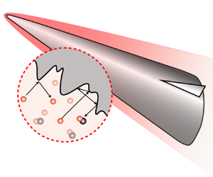
Hypersonic vehicles flying at high altitude are exposed to high-temperature and highly dissociated gases, and the gas–surface interactions such as catalysis, oxidation and energy accommodation show critical significance in evaluating the aerothermodynamic performance (Gnoffo Reference Gnoffo1999). The real surface of the vehicles is rough rather than smooth at different scales. In fact, besides that resulting from the manufacture precision, roughness due to the slight ablation or corrosion is also inevitable even for the so-called non-ablative thermal protection system designed for the new generation of cruising/gliding vehicles, as shown schematically in figure 1. In contrast to the macroscopic roughness, which usually alters the flow structure or leads to flow transition (Li & Dong Reference Li and Dong2021), the microscopic roughness is on the scale of the mean free path of the ambient gas molecules. Therefore, it will not directly change the macroscopic flow state, but could dramatically affect the heat and mass transport via the gas–surface interaction processes. As a result, it is necessary to understand the heterogeneously reacting flow over a wall with microscale roughness, and the rarefied gas effects could arise in the microstructure, although the flow past the vehicle is within the continuum regime. This problem is challenging since it is extremely costly, if not impossible, to either numerically or experimentally capture the detailed features in the microstructure.

Figure 1. The microscale roughness on the surface of a hypersonic vehicle.
A great many studies, as summarized by Bottaro (Reference Bottaro2019), can be found attacking the flow and transport problems involving a rough wall in various fields, for either theoretical interests or practical applications. Generally speaking, the transport problem raised by a rough wall can be attributed to solving the Laplace or Poisson equation in a domain with an oscillating boundary, which is a classical but hard problem in mathematics. Without a universal theoretical solution, many approximately analytical methods have been employed in specific situations. For the simplest one, the flow over a small amplitude wavy wall is usually solved by using the regular perturbation method as a typical example in textbooks (Van Dyke Reference Van Dyke1975). However, as the wave steepness is not small enough, mathematical singularity arises and more issues need to be considered, as studied by Amirat & Bodart (Reference Amirat and Bodart2001), Amirat et al. (Reference Amirat, Bodart, de Maio and Gaudiello2004); Amirat, Chechkin & Gadyl'shin (Reference Amirat, Chechkin and Gadyl'shin2006, Reference Amirat, Chechkin and Gadyl'shin2007) and Chechkin, Friedman & Piatnitski (Reference Chechkin, Friedman and Piatnitski1999). The conformal mapping method (Richardson Reference Richardson1973) has also been used to transfer the physical domain, especially that with an irregular or even fractal boundary (Mark Brady Reference Mark Brady1993; Blyth & Pozrikidis Reference Blyth and Pozrikidis2003), into a regular one which is then solved numerically. A more practical methodology is to introduce homogenization models (Sarkar & Prosperetti Reference Sarkar and Prosperetti1996; Nevard & Keller Reference Nevard and Keller1997; Achdou, Pironneau & Valentin Reference Achdou, Pironneau and Valentin1998; Bottaro Reference Bottaro2019) of rough walls, i.e. to replace the rough wall with an equivalent wall with effective wall properties. For example, Taylor (Reference Taylor1971) and Richardson (Reference Richardson1971, Reference Richardson1973) have discussed the slip boundary condition of the porous material walls. Bottaro (Reference Bottaro2019) has systematically reviewed and revisited the multiscale homogenization strategy in various flow problems. Usually, the previous studies considered only Dirichlet-type (first-type) and/or the Neumann-type (second-type) boundary conditions which apply to the shear stress and heat flux calculations. The relatively more complicated Robin-type (third-type) boundary condition which appears in surface reaction and mass transfer problems has not been discussed sufficiently, and the available studies are very rare. In addition, the rarefied gas effects are scarcely touched upon in these studies. Against this background, the present paper will specially discuss the surface reaction and mass transfer features of a thermal protection system covered by microstructures in which the rarefied gas effects could be significant.
The microstructure considered here, resulting from either the manufacture precision or slight ablation, has a scale much smaller than the thickness of the boundary layer (Song et al. Reference Song, Yang, Xin and Lu2018; Chung et al. Reference Chung, Hutchins, Schultz and Flack2021). Under the microscope, the morphology distribution usually has a periodicity with a characteristic dimension which, taking carbon-based materials (Panerai et al. Reference Panerai, Cochell, Martin and White2019; Levet et al. Reference Levet, Lachaud, Ducamp, Memes, Couzi, Mathiaud, Gillard, Weisbecker and Vignoles2021; Le, Ha & Goo Reference Le, Ha and Goo2021) as an example, depends on the diameter of carbon fibres, usually several micrometres (Vérant et al. Reference Vérant, Perron, Pichelin, Chazot, Kolesnikov, Sakharov, Gerasimova and Omaly2012). Despite its negligible effect on the macroscopic flow state, the increased wetted area and active sites show a positive effect on the surface reaction rate. This is why porous catalysts are so effective in chemical engineering (Hoogschagen Reference Hoogschagen1955).
On the other hand, for a typical hypersonic vehicle flying with a Mach number  $Ma_{\infty }\sim 20$ at an altitude in the range $40\unicode{x2013}50 {\rm km}$, the thickness of the boundary layer clinging to the leading edge is of the order of millimetres (Wang Reference Wang2014, p. 32), and the mean free path of molecules near the wall is micron sized, as shown in figure 1. As a result, the reaction and diffusion, as well as the incomplete energy accommodation process (Luo & Wang Reference Luo and Wang2020), in the roughness elements could be significantly influenced by the rarefied gas effects, as implied by the Knudsen number
 \begin{equation} Kn=\dfrac{\lambda}{L} , \end{equation}
where  $\lambda$ and $L$ denote the mean free path of molecules and the characteristic scale of the flow, respectively. In this work, there exist two flow scales, namely, the overall macroflow and the microflow within the roughness elements, and the Knudsen number defined for the latter is much larger than that for the former. As indicated by Massuti-Ballester & Herdrich (Reference Massuti-Ballester and Herdrich2021), a lack of awareness of the microscopic roughness is one of the main reasons causing the large scatter in the measurement data of materials’ thermochemical properties (Thoemel & Chazot Reference Thoemel and Chazot2009).
In fact, the diffusion in the microstructure could range between two limiting behaviours (Bird, Stewart & Lightfoot Reference Bird, Stewart and Lightfoot2002; Kavokine, Netz & Bocquet Reference Kavokine, Netz and Bocquet2021): bulk diffusion and Knudsen diffusion, corresponding to the continuum ( $Kn\ll 1$) and free molecular flow ( $Kn\gg 1$) cases, respectively. As in between ( $Kn\sim 1$), the slip and transition phenomena complicate the situation, and an effective diffusivity should be employed.
The homogeneous strategy of the rough wall should be tested in a typical and concise flow model which sufficiently reflects the multiscale characteristics we are concerned with and meanwhile filters out the unrelated factors. In most of the studies, the two-dimensional (2-D) roughness element is chosen for simplicity, and the results can be generalized to the three-dimensional (3-D) case (Achdou et al. Reference Achdou, Pironneau and Valentin1998). It is also shown by Nevard & Keller (Reference Nevard and Keller1997) that the effective boundary conditions determined by the solutions of certain special problems could also be extended to other problems with the same multiscale characteristics. Zhou et al. (Reference Zhou, Khayat, Martinuzzi and Straatman2002) found that the flow model based on a relatively simple geometry can exhibit many of the features present in much more complex geometries, which can significantly impact heat or mass transfer performance. Furthermore, the small perturbation caused by the roughness can be analysed in a linearized way. For the momentum transport problem, Wang (Reference Wang2003) showed that a parallel shear flow model adequately describes the fluid motion near the wall, regardless of the actual flow state being laminar or turbulent, as long as the size of the roughness is small enough compared with the nominal dimension of the macroscopic flow domain. For the heat transfer problem, Fyrillas & Pozrikidis (Reference Fyrillas and Pozrikidis2001) and Blyth & Pozrikidis (Reference Blyth and Pozrikidis2003) found that the curvature of the surface could be neglected, and the heat conduction dominates convection near the small-sized roughness, and the temperature field satisfies Laplace's equation to the leading-order approximation. For the surface reaction and diffusion problem, Ringhofer & Gobbert (Reference Ringhofer and Gobbert1998) stated that, for practical applications, the heat conduction and mass transfer can be treated separately, and thus the temperature is assumed to be a given quantity in their study in the reaction–diffusion process. They also adopted a realistic assumption of a constant and invariant roughness shape, considering that the growth of the surface is very slow compared with the characteristic flow time scale. Poovathingal & Schwartzentruber (Reference Poovathingal and Schwartzentruber2014) carried out a numerical study on the ablation process of a carbon-based surface, showing that the convection could be neglected in analysing an isolated roughness element.
Practically, a multiplying factor
 \begin{equation} \varPhi=\dfrac{k_{{w,r}}}{k_{{w,s}}} \end{equation}
can be used to evaluate the relative impact of the rough surface, where  $k_{{w,s}}$ is the reaction rate for smooth wall, and $k_{{w,r}}$ is the averaged reaction rate perceived by the macroscopic flow field in the presence of roughness over the same projected area. Here, $k_{{w,r}}$ is exactly the apparent or effective chemical property of the equivalent smooth wall in the corresponding homogeneous model, and it should depend both on the geometrical details of the roughness element and the flow state nearby. In principle, $\varPhi$ or $k_{{w,r}}$ can be obtained from molecular dynamics simulations (Poovathingal et al. Reference Poovathingal, Schwartzentruber, Srinivasan and van Duin2013) of the atomic-level interactions between the gas and the surface molecules, or from measurements of the mesoscopic/macroscopic property in the boundary layer. Many previous studies (Kim & Boudart Reference Kim and Boudart1991; Kim et al. Reference Kim, Lee, Kim and Park2020a; Kim, Yang & Park Reference Kim, Yang and Park2020b) showed that the multiplying factor increases proportionately with the roughness factor
 \begin{equation} R_{n}=\dfrac{A}{A_{0}}, \end{equation}
in a reasonable range of roughness, with  $A$ and $A_{0}$ being the wetted area and projected area of the roughness element, respectively. But this occurs only in the reaction-limited regime where the diffusion rate is much higher than the surface reaction rate. As the reaction rate increases and gradually dominates the diffusion rate, a diffusion-limited regime is approached and the effective rate of surface reactions will be decreased (Poovathingal & Schwartzentruber Reference Poovathingal and Schwartzentruber2014). Theoretical and quantitative modelling of this process is the main purpose of the present paper.
Inspired by the previous work, this paper proposed a quasi-one-dimensional (Q1-D) homogeneous model consisting of a macroscopic one-dimensional (1-D) surface reaction–diffusion model and a microscopic 2-D roughness model, with the latter embedded in the former as an effective boundary. The direct simulation Monte Carlo (DSMC) method is also employed to calibrate and validate the results within a practical range of flow parameters. The typical oxidizing reaction of the carbon-based surface (Poovathingal & Schwartzentruber Reference Poovathingal and Schwartzentruber2014) is considered in the analysis as an example because it is potentially associated with the formation of the roughness, but the conclusions are shown to also applicable to the catalytic reaction. Typical roughness geometries, varying rarefied flow regimes as well as reaction probabilities are taken into account. Effects of the flow and heat transfer are ignored at first in the theoretical analysis, and then recovered and evaluated at last in the numerical analysis. An extension to the 3-D roughness is also verified and discussed in the end.
2. Physical analysis and theoretical modelling
Following the convention of the previous work, the roughness element, i.e. the microstructure on the surface, should be embodied in a standard and practical flow model, in order to display its effects on the transport performance near the wall. A steady Q1-D surface reaction–diffusion model is introduced here to describe the flow features at distances that are large compared with the roughness but small compared with the nominal dimension, e.g. the boundary layer thickness, as shown in figure 2. The oxygen atoms enter from the outer boundary ( $y=H$) of the domain at a given concentration $X_\infty$ (and optionally at a given temperature $T_\infty$), and then diffuse towards the surface, which is named external diffusion. A nominal gas–surface reaction denoting the major reaction of carbon and ${\rm O}$ atoms (Poovathingal & Schwartzentruber Reference Poovathingal and Schwartzentruber2014; Murray et al. Reference Murray, Recio, Caracciolo, Miossec, Balucani, Casavecchia and Minton2020), ${{\rm C}({\rm s})+{\rm O} \rightarrow {\rm CO} }$, takes place on the surface placed at $y=0$ at a given temperature $T_{{w}}$. The released ${\rm CO}$ molecules diffuse towards the outer boundary and finally get away, this also being an external diffusion process. In the cavity of the roughness element, an internal diffusion exists, and the rarefied gas effects can play a role since the characteristic scale of the roughness is comparable to the mean free path of gas molecules, although the external flow could be within the continuum regime. The aim is to find a homogeneous equivalence of the rough wall to a smooth wall with effective chemical properties.

Figure 2. Schematic of the reaction–diffusion field near a wall. (a) Reaction–diffusion model of a rough surface. (b) Reaction–diffusion model of a smooth surface.
Without or with a tangential velocity, the model denotes the flow characteristics close to or downstream of the stagnation point. It will be shown later that the tangential velocity does not affect the equivalence, and so the tangential velocity is neglected at first. With regard to the normal velocity, it has two components: thermal velocity and bulk velocity. The thermal velocity is isotropous, but the bulk velocity is complex because diffusion will always produce convection (Cussler Reference Cussler2009) even in isothermal and isobaric systems. Fortunately, the convective velocity is zero if the molar average velocity is used in this problem. Furthermore, some assumptions need to be addressed:
(i) Gas-phase reaction has a much smaller extent than the surface reaction and therefore is neglected, which is in accordance with the traditional frozen boundary layer assumption in engineering practice and has been discussed in some previous studies (Poovathingal & Schwartzentruber Reference Poovathingal and Schwartzentruber2014). Certainly, the coupling and competition between the gas phase and heterogeneous reactions deserve future study.
(ii) Time-dependent interfacial motions are neglected here because the surface recession is slow as compared with the mass transfer (Lachaud et al. Reference Lachaud, Bertrand, Vignoles, Bourget, Rebillat and Weisbecker2007), and the flow is steady in this problem. A future analysis may consider the materials’ mass loss model such as the 1-D model proposed by Pirrone et al. (Reference Pirrone, Agabiti, Pagan and Herdrich2022).
(iii) The roughness elements have a period distribution, which is an abstraction of most practical surfaces (Panerai et al. Reference Panerai, Cochell, Martin and White2019; Levet et al. Reference Levet, Lachaud, Ducamp, Memes, Couzi, Mathiaud, Gillard, Weisbecker and Vignoles2021; Le et al. Reference Le, Ha and Goo2021).
(iv) The gas temperature, and therefore the property parameters, are constant within the microscale cavities even when the external flow field has a gradient, due to the small dimension of the surface roughness (Fyrillas & Pozrikidis Reference Fyrillas and Pozrikidis2001).
2.1. Reaction–diffusion induced by a smooth reactive wall
First, we need to have a clear understanding of the external surface reaction–diffusion above a smooth wall in order to subsequently test the internal surface reaction–diffusion model of the rough wall. As shown in figure 2(b), the 1-D flow field induced by a smooth reactive wall can be described by the heat conduction equation and mass diffusion equation (in molar units) in dimensionless form
 \begin{gather} \left. \begin{array}{ll@{}} \dfrac{{\rm{d}} }{{\rm{d}} \bar{y}}\left( \bar{K} \dfrac{{\rm{d}} \bar{T} }{{\rm{d}} \bar{y}}\right) =0 , & \\ \bar{T}= 1, & \bar{y}=1 ,\\ \bar{T}= Rt, & \bar{y}=0 ; \end{array} \right\} \end{gather}
 \begin{gather} \left. \begin{array}{ll@{}} \dfrac{{\rm{d}} }{{\rm{d}} \bar{y}}\left( \bar{n} \bar{D}_{{ij}} \dfrac{{\rm{d}} X }{{\rm{d}} \bar{y}}\right) =0 , & \\ X= X_\infty, & \bar{y}=1 , \\ \dfrac{{\rm{d}} X}{{\rm{d}} \bar{y}}=Da_{0} X, & \bar{y}=0 , \end{array} \right\} \end{gather}
where  $\bar {y}={y}/{H}$, with $H$ being the scale of the 1-D domain which is sufficiently small relative to the macroscopic flow scale and sufficiently large relative to the microscopic roughness scale, $Rt={T_{{w}}}/{T_{\infty }}$ and $X ={n_{(O)}}/{n}$ is the mole fraction of $\textrm {O}$ atoms. The temperature $T$, number density $n$, thermal conductivity $K$ and binary diffusion coefficient ${D}_{{ij}}$ are non-dimensionalized or normalized by their corresponding values at the outer boundary $\bar {y}=1$ (denoted by a subscript ‘ ${\infty }$’). In the first-order reaction boundary condition
 \begin{equation} Da_{0} = \dfrac{{k_{{w}}} H}{D_{{ij,w}}}, \end{equation}
is known as the Damköhler number (Inger Reference Inger2001), a non-equilibrium criterion that represents the relative speed of surface reaction and diffusion. Here,  $k_{{w}}$ is the surface reaction rate, and the subscript ‘ ${{w}}$’ denotes the properties at the wall.
At first appearance, the above equations seem very simple. However, even under the thermodynamic equilibrium assumption, the transport coefficients generally depend not only on the temperature, but also on the gas composition. As a result, (2.1) and (2.2) are coupled nonlinear equations for a gas mixture, and the solution process relies partly on the modelling of the mixture's physical properties.
According to the kinetic theory (Chapman & Cowling Reference Chapman and Cowling1990), the thermal conductivity for species ‘i’ is
 \begin{equation} K_{{i}}=c_{{i}} \dfrac{\sqrt{T/M_{{i}}}}{ \sigma^2_{{i}}\varOmega_{{K,i}}}. \end{equation}
For the gas mixture, there is Wilke's semiempirical rule (Bird et al. Reference Bird, Stewart and Lightfoot2002; Alkandry, Boyd & Martin Reference Alkandry, Boyd and Martin2014),  $K=\sum _{{i}}({X_{{i}}K_{{i}}}/{\phi _{{i}}})$ with the scaling factor
 \begin{equation} {\phi_{{i}}}=\sum_{{j}} X_{{j}}\left[ 1+\sqrt{\frac{K_{{i}}}{K_{{j}}}}\left( \frac{M_{{j}}}{M_{{i}}}\right)^{1/4} \right]^{2} \left[\sqrt{8\left(1+\frac{M_{{i}}}{M_{{j}}} \right) }\right]^{{-}1}. \end{equation}
By contrast, the binary diffusivity (Chapman & Cowling Reference Chapman and Cowling1990; Cussler Reference Cussler2009) takes the form
 \begin{equation} D_{{ij}}=c_{{ij}} \sqrt{T^3\left( \dfrac{1}{M_{{i}}}+\dfrac{1}{M_{{j}}}\right)} \dfrac{1}{p \sigma^2_{{ij}}\varOmega_{{D,ij}}}, \end{equation}
where  $M_{{i}}$ and $M_{{j}}$ are the molar mass of species ‘i’ and ‘j’, respectively, $p$ denotes the pressure, $\sigma$ is a characteristic diameter appearing in the molecular potential, and prefactors $c_{{i}}$ and $c_{{ij}}$ are the empirical coefficients. Also, $\varOmega _{{K,i}}$ and $\varOmega _{{D,ij}}$ are the collisional integrals for the thermal conduction and diffusion, respectively. The viscosity depends on the temperature with a power law $\mu \propto T^{\omega }$, with $\omega$ being the viscosity index and equal roughly to $0.75$ for most real gases (Bird Reference Bird1994). According to the similarity among the mass, momentum and energy transports, the collisional integrals for thermal conductivity and diffusivity conform to $\varOmega \propto T^{{1}/{2}-\omega }$ approximately. The diffusivity for the binary mixture $D_{{ij}}$ is almost independent of the composition (Bird et al. Reference Bird, Stewart and Lightfoot2002), and so we have $\bar {n}\bar {D}_{{ij}}\propto T^{\omega }$. Based on the thermal properties of molecular species provided by Miró Miró & Pinna (Reference Miró Miró and Pinna2021), it can be deduced that the complex relation between the thermal conductivity and the oxygen atoms’ mole concentration is approximately linear for the present gas mixture, i.e. $\bar {K} \propto \bar {T}^{\omega }(1+{\beta } X)$ with ${\beta } \approx 0.43$.
Now, (2.1) and (2.2) can be solved numerically, or alternatively, be analysed based on a perturbation idea since the coupling is relatively weak and the transport coefficients’ variation due to the temperature perturbation is slight. For the latter method, the zero-order solutions could be obtained without considering the coupling effects. Therefore, we get
 \begin{gather} \bar{T}_0=[ (1-{Rt}^{1+\omega})\bar{y} +{Rt}^{1+\omega}]^{{1}/({1+\omega})}, \end{gather}
 \begin{gather} \bar{X}_0=\frac{X_0}{X_\infty}=\frac{1+Da_0\bar{y}}{1+Da_0} . \end{gather}
The first-order solutions are then obtained by considering  $\bar {K} \propto \bar {T}^{\omega }(1+{\beta } X_0)$ and $\bar {n}\bar {D}_{{ij}}\propto T_0 ^{\omega }$ in (2.1) and (2.2). As a result,
 \begin{equation} \bar{T}_1 =\left[ \dfrac{\ln(1+c\bar{y})}{\ln(1+c)} ({1-{Rt}^{1+\omega}})+{Rt}^{1+\omega}\right]^{{1}/({1+\omega})}, \end{equation}
where  $c= {{\beta } Da_0}/({1+{\beta }+Da_0})$, and
 \begin{gather} \bar{X}_1=\frac{X_1}{X_\infty}=\dfrac{1+Da {\psi}(\bar{y})}{1+Da} , \end{gather}
 \begin{gather} {\psi}(\bar{y})=\dfrac{\left[ \left( \dfrac{1}{Rt^{1+\omega}} -1\right) \bar{y} +1\right]^{{1}/({1+\omega})}-1}{\dfrac{1}{Rt}-1}, \end{gather}
and the modified Damköhler number,
 \begin{equation} Da = \dfrac{1-Rt}{Rt^{-\omega}-Rt} \left(1+\omega \right) Da_{0} . \end{equation}
 The iteration process could go on in principle, but it will be shown later that the first-order approximation (2.10) is sufficient to predict the distribution of the mole concentration, while a higher-order approximation will introduce special complexity but negligible accuracy improvement. For the temperature distribution (2.9), a simple but efficient improvement could be supplemented by merely replacing  $Da_0$ in $c$ with the modified $Da$. Particularly, at the wall surface, $\bar {y}=0$ and $\psi (0)=0$, and we have
 \begin{equation} \bar{X}_{{w}}=\frac{X_{{w}}}{X_\infty}=\dfrac{1}{1+Da}. \end{equation}
 Now we consider a specific situation where the temperature of the entire flow field is uniform, i.e.  ${T_{\infty }}={T_{{w}}}$ and $Rt=1$. This a basic and effective model to discuss the diffusion and surface reaction problem. Based on L’H $\hat{\rm o}$pital’s rule, it is easy to derive that $Da=Da_{0}$, $\psi (\bar {y})=\bar {y}$ and the concentration profile (2.10) degrades into a linear form
 \begin{equation} \bar{X}=\frac{X}{X_\infty}=\dfrac{1+Da_0\bar{y}}{1+Da_0}. \end{equation}
The above linear formula (2.14) is adopted conveniently in the following theoretical analyses, but the more general (2.9) and (2.10) will also be displayed to show that the non-uniformity of the temperature does not affect the modelling of the roughness elements.
2.2. Rarefied gas effects
The analyses in the above subsection are still based on the continuum hypothesis, but as the microscopic phenomena are concerned, the rarefied gas effects should be evaluated and some corrections be introduced if necessary. For the present surface reaction–diffusion problem, corrections to the boundary conditions and diffusivity are particularly considered.
The no-slip boundary conditions assume the continuity of tangential velocity, temperature and the Gibbs chemical potentials across interfaces between phases. This is, however, a limiting case of the more general Navier partial-slip boundary conditions (Kavokine et al. Reference Kavokine, Netz and Bocquet2021). In view of the chemical non-equilibrium for multicomponent gases, the concentration slip boundary condition (Gupta, Scott & Moss Reference Gupta, Scott and Moss1985; Rosner & Papadopoulos Reference Rosner and Papadopoulos1996) is
 \begin{equation} X_{{slip}}=\dfrac{2-\gamma_{{i}}}{2\gamma_{{i}}} \sqrt{\dfrac{2 {\rm \pi}m_{{i}}}{k_{{B}}T_{{w}}}} D_{{ij}}\left. \dfrac{{\rm{d}} X}{{\rm{d}} {n}}\right|_{{w}}, \end{equation}
where  ${\textrm {{d}} [{\cdot }] }/{\textrm {{d}} {n}}$ means the gradient in the wall-normal direction, and $\gamma _{{i}}$, $k_{{B}}$ and $m_{{i}}$ are the surface reaction coefficient, Boltzmann constant and mass of the incident atom, respectively. The surface reaction coefficient $\gamma _{{i}}={N_{{react}}}/{N_{{tot}}}$ represents the probability of the oxidation reaction when an atom collides with the wall, with $N_{{tot}}$ being the total number flux of atoms impinging onto the surface and $N_{{react}}$ that reacting with the wall. Therefore, $\gamma _{{i}}$ takes a value between 0 and 1. Now, considering that the surface reaction rate
 \begin{equation} {k_{{w}}}=\dfrac{ 2\gamma_{{i}}}{2-\gamma_{{i}}}\sqrt{\dfrac{k_{{B}} T_{{w}}}{2{\rm \pi} m_{{i}} }} , \end{equation}
combining (2.15) and (2.16), we find
 \begin{equation} k_{{w}}X_{{slip}}=D_{{ij}}\left. \dfrac{{\rm{d}} X}{{\rm{d}} {n}}\right|_{{w}} , \end{equation}
which is the precisely first-order surface reaction. In other words, the slip boundary condition is equivalent to the first-order reaction boundary condition that has been adopted in (2.2).
It is worth noting that there is another popularly used expression for the surface reaction rate
 \begin{equation} {k_{{w}}}=\gamma_{{i}}\sqrt{\dfrac{k_{{B}} T_{{w}}}{2{\rm \pi} m_{{i}} }}. \end{equation}
In fact, there still exists an unresolved conflict for the two versions, i.e. (2.16) and (2.18). For a low reaction coefficient,  $\gamma _{{i}} <0.1$ for example, these two formulae are approximately equal, but for a high reaction probability, there is a non-physical jump between these two formulae. It is observed that (2.18) is commonly used in the continuum regime (Scott Reference Scott1992; Massuti-Ballester & Herdrich Reference Massuti-Ballester and Herdrich2017), and (2.16) in the rarefied regime (Gupta et al. Reference Gupta, Scott and Moss1985; Scott Reference Scott1992; Zade, Renksizbulut & Friedman Reference Zade, Renksizbulut and Friedman2008). Therefore (2.16) is more appropriate for the present rarefied gas condition, as will be confirmed later in our DSMC simulations which demonstrate a smooth transition from (2.18) to (2.16) as $\textit {Kn}$ increases.
Strictly speaking, the slip conditions also occur at the entrance to the flow domain. For example, in the DSMC simulation (Bird Reference Bird1994), the inflow boundary allows the inside molecules to cross the boundary to leave freely, and in the meantime, the stationary equilibrium gas atoms flow into the flow field. The number of inflow and outflow molecules will be equal so as to keep a steady state, which, at present, means a CO molecule flows out while an O atom flows in on average. Therefore, the entrance resembles a reduction wall where the reaction  ${\textrm {CO} \rightarrow \textrm {C}(\textrm {s})+\textrm {O} }$ occurs with a reaction coefficient $\gamma _\infty =1$. The no-slip Dirichlet boundary condition at $\bar {y}=1$ in (2.2) should be replaced by the slip Robin boundary condition
 \begin{equation} \dfrac{{\rm{d}} (1-X)}{{\rm{d}} \bar{y}} ={-}Da_{\infty}(1-X), \quad \bar{y}=1 , \end{equation}
where  $(1-X)$ is the molar concentration fraction of CO, and $Da_{\infty }= {{k_{\infty }}H}/{D_{{ij,\infty }}}$ is the Damköhler number defined based on the entrance parameters, with $k_{\infty }$ and $D_{{ij,\infty }}$ being the reaction rate and diffusivity at the entrance. Therefore, the concentration at the entrance is always less than unity, and a reciprocal relationship with (2.13) could be obtained as
 \begin{equation} 1-X_{\infty}=(1-X_{{w}})\dfrac{1}{1+Da_{\infty}}. \end{equation}
Finally, combining (2.13), (2.20) and (2.14), we get
 \begin{equation} {X}=X_{\infty}\dfrac{1+Da\bar{y}}{1+Da}=\dfrac{Da_{\infty}\left(1+ Da\bar{y}\right)}{Da+Da_{\infty}+DaDa_{\infty}}, \end{equation}
for a ‘completely reactive’ boundary condition at the entrance.
Actually, a coarse-grained estimation can be further given here to directly show the rarefied gas effects (denoting by  $Kn$) on the concentration distribution. Suppose an averaged pure gas, with diffusivity $D=\tfrac {1}{3} \bar {c} \lambda$ and mean thermal velocity $\bar {c}=\sqrt {{8k_{{B}}T}/{{\rm \pi} m}}$, according to the kinetic theory of gases
 \begin{equation} {k_{{w}}}=\frac{2\gamma_{{{i}}}}{2-\gamma_{{{i}}}}\sqrt{\frac{k_{{B}} T_{{w}}}{2{\rm \pi} m }} = \frac{2\gamma_{{{i}}}}{2-\gamma_{{{i}}}} \frac{\bar{c}}{4}\quad {\rm and}\quad {{k_{\infty}}}=2\sqrt{\frac{k_{{B}} T_{{w}}}{2{\rm \pi} m }}, \end{equation}
as the imaginary reaction coefficient is unity at the entrance. As a result, the Damköhler number is inversely proportional to the Knudsen number, i.e.
 \begin{equation} Da=\frac{{k_{{w}}} H}{D} =\frac{\gamma_{{{i}}}}{2-\gamma_{{{i}}}}\frac{3H}{2\lambda}= \frac{\gamma_{{{i}}}}{2-\gamma_{{{i}}}}\frac{3}{2Kn}, \end{equation}
and similarly, we get  $Da_{\infty }= {3}/{2Kn}$ from $\gamma _{\infty }=1$. Equation (2.21) can be rewritten as
 \begin{equation} X=\dfrac{2(2-\gamma_{{{i}}})Kn+3\gamma_{{{i}}}\bar{y}}{4Kn+3\gamma_{{{i}}}}. \end{equation}
A degraded version of (2.24) has been reported by Rosner & Papadopoulos (Reference Rosner and Papadopoulos1996) and Xu & Ju (Reference Xu and Ju2005) who further assumed  $\gamma _{{{i}}}=1$, and used (2.18) rather than (2.16).
Besides the slip effects on the boundaries, the rarefied gas effects also emerge in the flow field as  $Kn$ increases. Actually, the diffusion feature deviates from the bulk diffusion, and there appears a complex behaviour in the transition flow regime. Due to a lack of precise description, a popular and convenient treatment (Keerthi et al. Reference Keerthi2018) is to assume that Fick's first law still works even in the high $Kn$ regime and to replace the bulk diffusivity with an empirical formula such as Bosanquet's relation (Hewitt & Sharratt Reference Hewitt and Sharratt1963; Zalc, Reyes & Iglesia Reference Zalc, Reyes and Iglesia2004; Lachaud, Cozmuta & Mansour Reference Lachaud, Cozmuta and Mansour2010; Achambath & Schwartzentruber Reference Achambath and Schwartzentruber2018)
 \begin{equation} D=\left( \dfrac{1}{D_{Kn} }+\dfrac{1}{D_{{ij}}}\right) ^{{-}1} , \end{equation}
where  $D$ is the effective diffusivity, $D_{Kn}$ is the Knudsen diffusivity (Present Reference Present1958; Shindo et al. Reference Shindo, Hakuta, Yoshitome and Inoue1983; Levdanskii et al. Reference Levdanskii, Roldugin, Zhdanov and Zdimal2014; Kavokine et al. Reference Kavokine, Netz and Bocquet2021) and $D_{{ij}}/D_{Kn} \propto \lambda /L = Kn$.
In the continuum regime,  $Kn \ll 1$, and $D \approx D_{{ij}}$. Inversely, for the free molecular flow, $Kn \gg 1$, and $D \approx D_{Kn}$, which means the gas–surface collisions dominate collisions between gas molecules. The diffusivity correction in the external diffusion region is probably not so significant, but in the internal diffusion region of the roughness, the flow is generally highly rarefied and the Knudsen diffusion is the primary mechanism. To avoid getting too far off the main topic, a detailed discussion of the Knudsen diffusivity can be found in Appendix A.
2.3. Diffusion–reaction induced by a rough surface
The diffusion–reaction effects of the roughness can be decoupled from the external flow region as its size is sufficiently small compared with the characteristic scale of the macroscopic flow. Difficulties arise from the complex geometries of the boundaries and the porosity. Pragmatically, the effect of various actual roughness geometries could be related to that of some standard ones under the same flow conditions, as has been seen for the equivalent sand roughness model (Sigal & Danberg Reference Sigal and Danberg1990; Hermann Schlichting Reference Hermann Schlichting2017) which has been popularly used in engineering practice. Therefore, two typical geometries, the rectangle and the triangle, are particularly considered here, and it will be shown later that the method and conclusion apply also to even the 3-D roughness elements.
The mass diffusion in a roughness pore is similar to the heat transfer in the same region, and the analogy between diffusion and heat transfer could be used to model the interaction of diffusion and reaction in the cavities, with the assumptions in § 2 similar to the Murray–Gardner assumptions (Kraus, Aziz & Welty Reference Kraus, Aziz and Welty2001, p. 10) for the heat transfer in fins. For the Q1-D flow field, an imaginary plane is aligned with the peak of the morphology ( $y=0$) without loss of generality, and the concentration fraction in volume at the plane is set to an arbitrary constant $X_{{e}}$. As the mean free path of the gas molecules is comparable to the characteristic dimension of the pores, the corresponding binary diffusivity $D_{{ij}}$ should be replaced by the effective diffusivity $D$ in (2.25).
2.3.1. Rectangular roughness surface
Considering a rough wall modelled by an array of rectangular modules, as shown in figure 3, the characteristic dimension contains the projected length  $A_{0}$ (projected area for 3-D roughness), the width of the pore $d$ and depth $h$ and the roughness factor is $R_{n}={A}/{A_{0}}=1+{2h}/{A_{0}}$. The concentration distribution satisfies the 2-D Laplace equation, the exact analytical solution is an infinite sine and cosine series, but the boundary geometrical morphology makes the solution too complex to apply in practice. In comparison, for the longitudinal structures, or when the internal reaction is not too much faster than the diffusion (Jochen Reference Jochen1997), the 1-D approximate equation is easier and sufficient (Kraus et al. Reference Kraus, Aziz and Welty2001, p. 702). As the total mass flux in the $y$ direction is concerned, $N_{{in}}-N_{{out}}=n D ({\textrm {{d}}^2 {X}}/{\textrm {{d}} {y}^2}) d =2nk_{{w}}X$, the non-dimensional equations can be easily written as follows (Lachaud et al. Reference Lachaud, Bertrand, Vignoles, Bourget, Rebillat and Weisbecker2007):
 \begin{equation} \left. \begin{array}{ll@{}} \dfrac{{\rm{d}}^2\tilde{X}}{{\rm{d}} {\xi}^2}={\textit{Th}}^2 \delta^2\tilde{X}, & \\ \tilde{X}=1, & \xi=0 ,\\ \dfrac{{\rm{d}} \tilde{X}}{{\rm{d}} \xi}={-}\dfrac{\textit{Th} ^{2}\delta}{2} \tilde{X}, & \xi=1 , \end{array} \right\} \end{equation}
in which  $\tilde {X}={X}/{X_{{e}}}$, $\xi =-({y}/{h})$ and $\delta ={h}/{d}$. The Thiele number (Achambath & Schwartzentruber Reference Achambath and Schwartzentruber2018) ${Th}=\sqrt {{2k_{{w}} {d}}/{D}}$, similar to the Damköhler number defined for the external flow, represents the relative influence of the reaction compared with the diffusion in the internal diffusion flow. The solution of (2.26) is
 \begin{equation} \tilde{X}=\cosh(\textit{Th} \delta \xi )-\sinh (\textit{Th} \delta \xi) {S}_{{rect}} , \end{equation}
with
 \begin{equation} S_{{rect}}=\dfrac{\dfrac{\textit{Th}}{2} \cosh(\textit{Th}\delta ) + \sinh(\textit{Th}\delta)}{ \cosh(\textit{Th} \delta ) +\dfrac{\textit{Th}}{2} \sinh( \textit{Th}\delta )} . \end{equation}
Figure 3. Schematic of the rectangular roughness.
2.3.2. Triangular roughness surface
Figure 4 displays a triangular roughness element. It is apparent that  $d =2h \tan {\theta }$ with $\theta$ being the semiangle, and the roughness factor $R_{n}={A}/{A_{0}}={1}/{\sin {\theta }}=\sqrt {1+4{\delta }^2}$. The governing equation is the generalized Bessel equation
 \begin{equation} \left. \begin{aligned} & (1-\xi) \dfrac{{\rm{d}}^2\tilde{X}}{{\rm{d}} {\xi}^{2}} -\dfrac{{\rm{d}} \tilde{X}}{{\rm{d}} {\xi }} =\dfrac{{\textit{Th}}^{2}\delta}{ 2 \sin{\theta}}\tilde{X} ,\\ & \tilde{X}=1, \quad \xi=0 ,\\ & \tilde{X}< \infty, \quad \xi=1 , \end{aligned} \right\} \end{equation}
where  $\textit {Th}=\sqrt {{2k_{{w}} {d} }/{D}}$ is the Thiele number the same as that for the rectangular roughness. The solution is expressible as a Bessel function
 \begin{equation} \tilde{X} = \dfrac{{\rm I}_{0}\left( \textit{Th} \textit{S}_{{tri}} \sqrt{(1-\xi)} \right) }{ {\rm I}_{0}\left( \textit{Th} \textit{S}_{{tri}} \right)} , \end{equation}
where  $\textit {S}_{{tri}}=\sqrt {{2\delta }/{\sin {\theta }}}$, and $\textrm {I}_0$ is the zero-order modified Bessel function of the first kind.

Figure 4. Schematic of the triangular roughness.
2.3.3. Effect of the surface roughness
As discussed above, the effect of the rough wall with an intrinsic reaction rate  $k_{{w}}$ is expected to be equivalent to a virtual smooth wall with an effective reaction rate $\varPhi k_{{w}}$. The number flux reacting at the virtual wall is
 \begin{equation} N_{{react}}=n X_{{e}} \varPhi k_{{w}}, \end{equation}
while the number flux diffusion to the wall is
 \begin{equation} N_{{in}}=n X_{{e}} D\dfrac{{\rm{d}} \tilde{X}}{{\rm{d}} {{y}}}. \end{equation}
Since  $N_{{react}}=N_{{in}}$, we have $\varPhi k_{{w}}=D({\textrm {{d}} \tilde {X}}/{\textrm {{d}} {\textit {y}}})|_{y=0}=D({\textrm {{d}} \tilde {X}}/{\textrm {{d}} {\xi }})({\textrm {{d}} \xi }/{\textrm {{d}} {\textit {y}}})|_{\xi =0}$, and thus
 \begin{equation} \varPhi=\left.-\dfrac{D}{k_{{w}}h}\dfrac{{\rm{d}} \tilde{X}}{{\rm{d}} {\xi}} \right|_{\xi=0}=\left.-\dfrac{2}{Th^2 \delta}\dfrac{{\rm{d}} \tilde{X}}{{\rm{d}} {\xi}}\right|_{\xi=0}. \end{equation}
Here,  $\varphi$ is introduced to represent the multiplying factor in the pore, while $\varPhi$ is for the whole rough wall accounting for the influence of the surface porosity. With the concentration distributions (2.27) and (2.30) in the microstructures, (2.33) can be rewritten as
 \begin{equation} \varphi_{{rect}}= \dfrac{2\textit{S}_{{rect}}}{\textit{Th}} \end{equation}
for the rectangular roughness, and
 \begin{equation} \varphi_{{tri}} =\dfrac{\textit{S}_{{tri}}}{\textit{Th} \delta} \dfrac{{\rm I}_{1}\left( \textit{Th} \textit{S}_{{tri}}\right) }{{\rm I}_{0}\left( \textit{Th} \textit{S}_{{tri}}\right)} \end{equation}
for the triangular roughness, where  $\textrm {I}_1$ is the first-order modified Bessel function of the first kind.
For ease of application, the asymptotic approximations can be derived by considering the dominated factors. For the rectangular roughness element, when  $\textit {Th}\delta$ is small, the process is limited by the surface reaction, and $\textit {S}_{{rect}}\approx {Th}/{2}+Th\delta$. On the contrary, when $\textit {Th}\delta$ is large, the process is limited by the diffusion, and $\textit {S}_{{rect}}\approx 1$. Besides, when $\textit {Th} \delta \simeq 1$, $\varphi$ can be approximated by its first-order Taylor expansion. Therefore, $\varphi _{{rect}}$ can be classified into three regimes naturally
 \begin{equation} \varphi_{{rect}}=\left\{\begin{array}{ll@{}} 1+2\delta, & \textit{Th}{\delta} <0.4 ,\\ \dfrac{6+12{\delta}+2Th^2 {\delta}^2 }{6+3Th^2 \delta+2Th^2 {\delta}^2 } , & 0.4 \leq \textit{Th} {\delta} < 2 ,\\ \dfrac{2}{\textit{Th}} , & \textit{Th}{\delta} \geq 2 . \end{array} \right. \end{equation}
Here,  $\varphi _{{rect}} \approx 1+2\delta$ is identical to the roughness factor $R_{n}$ when the reaction is slow enough, which is consistent with the results of references (Kim & Boudart Reference Kim and Boudart1991; Kim et al. Reference Kim, Lee, Kim and Park2020a,Reference Kim, Yang and Parkb). Specially, we find $\varphi _{{rect}} \simeq 1$ as $\textit {Th}=2$, indicating that the effect of roughness will vanish at $\textit {Th}=2$, whether the depth $\delta$ is small or large. What is more interesting is that the microstructure may even decrease the reaction rate when $Th>2$, and this finding is in agreement with the numerical simulations of Poovathingal & Schwartzentruber (Reference Poovathingal and Schwartzentruber2014).
Moreover, for more subtle nanopores or a very rarefied atmosphere, the local Knudsen number  $Kn_{{L}}={ \lambda }/{d}\gg 1$, the transport is dominated by the Knudsen diffusion and the diffusivity $D \propto \bar {c} d$ with a proportionality factor a little smaller than $2/3$. Then we have $\textit {Th}=\sqrt {{2k_{{w}}{d}}/{D}} \propto \sqrt {{\gamma _{{i}}}/({2-\gamma _{{i}}})}$ with a proportionality factor around $2$, indicating that $\textit {Th}$ almost depends completely on $\gamma _{{i}}$. As a result, $\textit {Th}\approx 2$ and $\varPhi _{{rect}} \approx 1$ when $\gamma _{{i}} =1$. Physically speaking, the result precisely corresponds to the fact that the reactant should be fully reacted on either the smooth or the rough wall.
For the triangular roughness, a similar classification yields
 \begin{equation} \varphi_{{tri}}=\left\{\begin{array}{ll@{}} \dfrac{1}{\sin{\theta}}, & \textit{Th} \textit{S}_{{tri}}<0.4 ,\\ \dfrac{2}{\sin{\theta}}\left(0.54-0.1Th\textit{S}_{{tri}} \right) , & 0.4\leq \textit{Th} \textit{S}_{{tri}}< 2 ,\\ \dfrac{\textit{S}_{{tri}}}{\textit{Th}\delta}\approx \dfrac{2}{\textit{Th}} , & \textit{Th} \textit{S}_{{tri}} \geq 2 . \end{array} \right. \end{equation}
When the reaction is much slower than the diffusion,  $\varphi _{{tri}} ={1}/{\sin {\theta }}$, equal to the roughness factor $R_{n}$ as expected. When the process is reaction limited and the pore structure is narrow, $\textit {S}_{{tri}} \approx 2\delta$ and $\varphi _{{tri}}={2}/{\textit {Th}}$, arriving at a consensus on the asymptotic form for large or small Thiele number in (2.36).
2.3.4. Influence of the surface porosity
The above discussion only considers the internal reaction in the microstructure, i.e. a limiting case for the surface porosity
 \begin{equation} \epsilon=\dfrac{d}{A_0} , \end{equation}
which is a key factor of the performance of materials (Sing Reference Sing1985). In a single period, the microstructure contains a pore of width  $d$ and platform of width $(A_0-d)$ as shown in figure 3. The platform has the same performance as a smooth wall, and therefore, the overall influence of surface roughness can be considered as the combination of these two parts,
 \begin{equation} \varPhi=1+\epsilon \left( \varphi-1\right). \end{equation}
 Considering a narrow pore structure, namely  $\epsilon \ll 1$, therefore $\varPhi \approx 1$. This indicates that although an isolated microscale structure could bring a non-negligible roughness factor $R_{n}$, it has an insignificant effect on the surface reaction characteristics.
3. Validations and discussions
3.1. Details of the numerical simulations
To validate the above theoretical analysis, a series of DSMC results is provided from the open-source DS2V (Bird Reference Bird2005) program which has been popularly used and well verified in this community and is acknowledged to be reliable in simulating rarefied and non-equilibrium flows. In the simulation, Maxwell's diffuse reflection boundary condition is adopted, and the momentum and energy accommodation coefficients are both set to 1. The variable soft sphere model (Bird Reference Bird1994) is used to treat the molecular collisions, and the parameters are shown in table 1. The molecular model parameters are significant in studying the transport properties of high-temperature gas, and many researchers (Swaminathan-Gopalan & Stephani Reference Swaminathan-Gopalan and Stephani2016) have devoted efforts to providing various fitting data for different temperature ranges in practical application. However, it does not matter which parameters or even model are used, and the present modelling study, as well as the dimensionless results, holds its validity, since the model parameters merely quantitatively affect the dimensional diffusion coefficient. We have found that, for the flow conditions in the current work, the results based on the variable hard sphere model show an insignificant deviation from those based on the variable soft sphere model. Despite that, it is recommended that the variable soft sphere model with suitable fitting parameters should be used in simulation of practical high-temperature flow involving significant mass diffusion effects.
Table 1. Molecular parameters in the DSMC simulations ( $T_{{ref}}=300\,\textrm {K}$).

In the DS2V program, the time step is approximately 1/3 of the mean collision time, and it is checked in the program automatically. The mesh is automatically generated and locally adapted; the default setting ensures that each cell contains more than eight particles, and the cell size is smaller than 1/3 of the mean free path in all simulations. If the degree of rarefaction is high, more particles, as well as more cells, are needed to reduce the statistical dispersion (Bhagat, Gijare & Dongari Reference Bhagat, Gijare and Dongari2019), and in this study, there are approximately 3 million particles and more than 100 thousand collision cells in a typical simulation. We have verified that the present setting of the cell size and particle number per cell is reasonable for a credible DSMC simulation.
In this section, two aspects of the theoretical modelling, i.e. results of the external flow and the internal flow need to be validated separately. There are four groups of simulation cases categorized according to different conditions, as listed in table 2. Group A contains a series of simulations for the smooth wall to validate the analytical results of the external surface reaction–diffusion, and it acts as a baseline to evaluate the effect of the roughness.
Table 2. Parameters in the DSMC simulations.

The baseline simulation is conducted under the flow condition with the bulk velocity  $0\,\textrm {m}\,\textrm {s}^{-1}$, temperature $300\,\textrm {K}$ and number density of oxygen atoms ${10}^{24}\,\textrm {m}^{-3}$. The inflow is prescribed at $y=H=500\,\mathrm {\mu }\textrm {m}$, the reactive carbon wall is placed at $y=0\, \mathrm {\mu }\textrm {m}$ and the periodic boundary condition is used in the $x$ direction, as presented in figure 2. The reaction coefficient varies from 0 to 1, namely, $\gamma _{{i}}=$ 0.001, 0.01, 0.1, 0.2, 0.5 and 1. Besides, two kinds of roughness geometry are set in group B, to indicate the effects of the roughness geometry, roughness factor $R_{n}$ and surface porosity. Group C has the same roughness as group B, but a shear velocity and a temperature gradient are taken into consideration. In group D, as an extension of the theories for the oxidation reaction, the catalytic reaction ${\textrm {O}+\textrm {O} \rightarrow \textrm {O}_2 }$ is simulated to assess the effects of roughness on catalysis.
3.1.1. Reaction–diffusion performance of a smooth surface
First, the concentration profiles with variable Damköhler numbers  $Da$ are displayed in figure 5, where $\gamma _{\infty } =1$ has been assumed and two typical values of $Da_\infty$ are demonstrated. A good agreement between the DSMC results and the theoretical predictions by (2.21) can be observed. As $\gamma =1$ is also adopted, a special version of (2.24) shows a direct dependence of the concentration profile on the Knudsen number, i.e. $X=({2Kn+3\bar {y}})/({4Kn+3})$, which is also compared with the DSMC results in figure 6, indicating that the concentration profile remains essentially linear in the entire flow regime. The above two figures demonstrate that the first-order slip model is sufficient to predict the concentration slip here. A distinct concentration slip can be observed when $Kn_{\infty } >0.05$, and formula (2.15) is approximately accurate in the slip regime, but with the increase of $\textit {Kn}$ number, (2.21) with the correction of Bosanquet's relation works better. It is interesting to note that all the profile lines in figure 6 intersect at $\bar {y}=0.43$ and $\bar {X}=43\,\%$. The reason is that CO molecule is heavier than the O atom, and the mean thermal velocity and thus Damköhler number are inversely proportional to the square root of the mass, i.e. ${Da}/{Da^{'}}=\sqrt {{m_{{CO}}}/{m_{{O}}}}=\sqrt {{28}/{16}}$, leading to an immovable point $\bar {X}=\bar {y}={1}/({1+\sqrt {{28}/{16}}}) \approx 0.43$.

Figure 5. Concentration profiles of oxygen atom under different non-equilibrium degrees (symbols: DSMC results in group A; lines: theoretical predictions by (2.21)); (a)  $Kn_{\infty }=0.005$ and $Da_{\infty }=177.3$, (b) $Kn_{\infty }=0.5$ and $Da_{\infty }=2.34$.

Figure 6. Concentration profiles under different rarefaction degrees (symbols: DSMC results in group A; lines: theoretical predictions by (2.21)).
It is also interesting to rationalize our use of (2.16). While the reaction probability  $\gamma$ is directly set in the simulation, the reaction rate $k_{{w}}$ could be deduced from the DSMC results by using (2.21) and (2.3) successively. Figure 7 shows the relation between $k_{{w}}$ and $\gamma$ under various Knudsen numbers. The DSMC results vary smoothly between the two limits, from (2.18) to (2.16), as the flow becomes rarefied. This comparison vividly clarifies the confusion of different expressions for the reaction rate in the literature.

Figure 7. The relation between the reaction rate  $k_{{w}}$ and the reaction coefficient $\gamma$ (group A).
Figure 8(a) shows the temperature profiles in the non-isothermal situation, and figure 8(b) shows the concentration profiles under different reaction rates when  $T_{\infty }=2000\,\textrm {K}$. It is found that as a large temperature difference is imposed, both the temperature and concentration distributions show apparent nonlinearities. However, the analytical first-order approximations are appropriate for the corresponding predictions under various practical conditions.

Figure 8. Temperature (a) profiles ( $\gamma =0.1$) (symbols: DSMC results in group A, $Kn_{\infty }=0.005$; dashed lines: zero-order approximation (2.7); solid lines: first-order approximation (2.9)) and concentration (b) profiles ( $T_{\infty }=2000\,\textrm {K}$) (solid lines: first-order approximation (2.10)) in a non-isothermal flow field.
3.2. Reaction–diffusive around a roughness element
For a smooth wall, the reaction rate  $k_{{w}}$ depends only on $\gamma$, but for a rough wall, the apparent reaction rate is also related to the morphological features. Figure 9 displays the concentration contours near the rough wall, and it is observed that the horizontal variation of the concentration is slight relative to the longitudinal variation, and a 1-D approximation is reasonable for either the internal or external region of the pore. The reasonableness could be further testified by the concentration profiles along three typical lines extracted from the flow field, and as shown in the figure, the consistency among them is quite satisfactory. The analytical prediction of the concentration distribution in the pore is provided by (2.27), and that outside the pore is provided by (2.21) with the apparent surface reaction rate determined by (2.39). A distinct inflection point can be observed at $y=0$, and the maximum relative error is less than 5 % at $y=0$, which provides a visualized validation of the Q1-D theoretical modelling in this study.


It is important to reiterate that the multiplying factor  $\varPhi$ is a key factor used to quantitatively compare the impact of the roughness. The results are summarized in figures 10 and 11 for the rectangular and triangular roughness elements, respectively, with the local Knudsen number $\textit {Kn}_{{L}}=\lambda /d$ varying up to five orders of magnitude. In general, as $\gamma$ increases, $\varPhi$ will decrease to even less than 1, indicating that the roughness will retard rather than accelerate the reaction when the process is diffusion limited. This performance corresponds to the fact that molecules in the microstructure block the atoms and prevent them from colliding with the wall, and the reactant and product cannot transport through the pore in time, leading to a reduction of the overall reaction rate in the microstructure. When $\textit {Kn}_{{L}} \gg 1$, the Knudsen diffusion is dominant, $\varPhi =R_n$ when $\gamma \ll 1$, and $\varPhi =1$ when $\gamma =1$, as discussed in the above section. It is notable that the diffusivity (2.25) and then the multiplying factor $\varPhi$ decrease continuously with the decrease of $\textit {Kn}$.

Figure 10. Multiplying factor for the rectangular roughness (group B,  $\epsilon =\tfrac {1}{2}$); (a) $R_n=1.414$, (b) $R_n=2$, (c) $R_n=3$.

Figure 11. Multiplying factor for the triangular roughness (group B,  $\epsilon =1$); (a) $R_n=1.414$, (b) $R_n=2$, (c) $R_n=3$.
Furthermore, the separate curves in figure 10 can be described by the characteristic parameter  $Th$ in a normalized curve, as shown in figure 12(a), where the solid line represents the theoretical prediction of (2.34), and the three approximate segments (S1–S3) represent the asymptotic predictions of (2.36). Similarly, the corresponding features of the triangular roughness are plotted in figure 12(b). Figure 13 shows the slight difference between effects of the rectangle and triangular roughness with consideration of the surface porosity (2.39). It is apparent that both of the roughness geometries exhibit a similar pattern, with the multiplying factor of the rectangular roughness only a little higher than that of the triangular roughness. However, lines of the rectangular and triangular roughnesses arrive at a consensus for large $Th$, as anticipated. The considerable consistency has practical meaning, since it indicates the potential that the present results could be extended to other roughness structures without major corrections.

Figure 12. Dependence of  $\varPhi$ on $\textit {Th}$ number (group B, $R_n=2$; theory lines predicted by (2.34) and (2.35); approximation S1–S3 predicted by (2.36) and (2.37)); (a) $\varPhi$ for the rectangular roughness $(\epsilon =\tfrac {1}{2})$, (b) $\varPhi$ for the triangular roughness ( $\epsilon =1$).

Figure 13. The influence of surface porosity (group B,  $\epsilon =1, 0.5, 0.25$; symbols: DSMC results; lines: theoretical predictions by (2.39)).
3.3. Equivalence of a rough wall to a smooth wall
The above discussion verified  $\varPhi$ under various conditions, and the reasonableness of the equivalent wall will be discussed here. Therefore, group C in table 2 is used to discuss the equivalence of a rough wall to a smooth wall. Three simulations are performed; first, a smooth wall with the intrinsic reaction coefficient $\gamma =0.01$, second, a rough wall with the same reaction coefficient and, third, a smooth wall with an effective reaction rate $\gamma _{{eff}}\approx 0.0284$, since (2.39) predicts $\varPhi \approx 2.84$. The first simulation is a baseline, the second is the actual situation while the third demonstrates the practical value of the present theoretical modelling, as shown in figure 14 for the isothermal case and in figure 15 for the non-isothermal case. The concentration distribution is significantly affected by the roughness, but the analytical formulae introduced here provide a nearly perfect correction. For the non-isothermal case, all the simulated temperature profiles are in good agreement with the theoretical predictions, indicating that the temperature of the gas is not directly influenced by the roughness since the gaseous reaction is ignored currently.

Figure 14. Concentration profiles for a rough wall and the equivalent smooth wall (symbols: DSMC results in group C,  $Kn_{\infty }=0.005$; lines: theoretical predictions by (2.21)).

Figure 15. Temperature and concentration profiles for a rough wall and the equivalent smooth wall with an effective reaction coefficient (symbols: DSMC results in group C ,  $Kn_{\infty }=0.005$; lines: theoretical predictions of temperature and concentration by (2.9) and (2.10), respectively). (a) Temperature profiles ( $T_{\infty }=2000\,\textrm {K}$). (b) Concentration profiles.
Figure 15 shows the temperature and concentration profiles in a non-isothermal condition. All three temperature profiles are in good agreement with the theory lines which are predicted by (2.9). The concentration distribution of the equivalent smooth wall is in line with the data from the rough wall, as anticipated.
Although the analytical results in this study were derived under the assumption of zero tangential velocity, it was inferred physically that they ought to be extended to the flow with a shear velocity. Therefore, group C in table 2 also includes cases to check the influence of the shear velocity. The bulk velocity in the  $x$ direction is set to be $1000\,\textrm {m}\,\textrm {s}^{-1}$, and the velocity gradient is $2 \times 10^{6} \,\textrm {s}^{-1}$, showing a typical strong shear characteristic. As shown in figure 16, the simulations are performed as the same as figure 15 except for the addition of the tangential velocity. The temperature profile diverges slightly from the prediction of (2.9) due to the viscous dissipation effect of the shear flow. The velocity slip and temperature jump are barely discernible under this condition, since $Kn_{\infty }$ is still small enough and the accommodation coefficients of momentum and energy are set to 1. If the incomplete accommodation phenomenon (accommodation coefficient less than 1) is specially of concern in other problems, it is speculated that by using the idea in this study, similar corrections could be introduced for the velocity slip and temperature jump boundary conditions.


These results indicate that the roughness has ignorable effects on the temperature and velocity distributions, echoing our inference at the beginning, namely, the microscale roughness will not directly alter the macroscopic flow structure. As a result, the reacting flow over a rough wall can be equivalent to that over a smooth wall with an effective surface property, even with a large temperature difference and a high shear velocity. In addition, various models of the velocity slip and temperature jump can be used on the virtual smooth wall like in other places.
3.4. Extension to the catalysis reaction
Heterogeneous catalysis ( ${\textrm {O}+\textrm {O} \rightarrow \textrm {O}_2 }$) is another surface reaction that is very important in hypersonic aerothermodynamics, and it affects the aerodynamic heating rate significantly (Zhang & Wang Reference Zhang and Wang2022). Qualitatively, it is similarly affected by the surface roughness, but quantitatively, there are significant differences between the oxidation and catalysis reactions. The concentration distribution in a corresponding isothermal catalysis reaction–diffusion problem can be got from Bird's monograph (Bird et al. Reference Bird, Stewart and Lightfoot2002, p. 553), namely,
 \begin{equation} 1-\dfrac{1}{2}\bar{X}=\dfrac{1}{2^{\bar{y}}}\left( 1-\dfrac{1}{2}\bar{X}_{{w}}\right)^{1-\bar{y}}, \end{equation}
where  $\bar {X}_{{w}}$ is the concentration at the surface $(\bar {y}=0)$, and
 \begin{equation} \bar{X}_{{w}}=\dfrac{2}{Da}\ln{(2-\bar{X}_{{w}})}. \end{equation}
This is a transcendental equation, but it is easy to get a numerical solution, where  $Da={{k_{{w}}} H}/{D_{{ij,w}}}$ is formally as same as that for the oxidation reactions. The simulations in group D of table 2 are intended to explore the influence of the roughness on the surface catalysis. As before, three simulations are performed, and two analytical predictions from (3.1), one with the intrinsic reaction rate and the other with the effective one, are shown and compared in figure 17. It can be seen that the theoretical results are in good agreements with the DSMC simulations, and the correction based on the multiplying factor $\varPhi$ works very well.

Figure 17. Concentration profiles for the catalysis reaction and diffusion problem (symbols: DSMC results in group D,  $Kn_{\infty }=0.005$; lines: theory by (3.1)).
Moreover, we consider some engineering-type materials like carbon fibre reinforced composite on which the depth of cavities may be much larger than the diameter (Levet et al. Reference Levet, Helber, Couzi, Mathiaud, Gouriet, Chazot and Vignoles2017). Thoemel & Chazot (Reference Thoemel and Chazot2009) did a series of catalytic reaction simulations where the pore diameter  $d$ was fixed, but the pore depth varied to increase the surface area. In this microstructure, $Th$ can be approximately regarded as fixed by the pore diameter, and it is inferred from limited information that $Th$ is around $0.1$. The results are illustrated in figure 18 where the lines are predicted by (2.34), and the symbols are from simulations of Thoemel & Chazot (Reference Thoemel and Chazot2009). The figure also shows the experimental data of Kim & Boudart (Reference Kim and Boudart1991) where the 3-D roughness was produced by the silica powder in a fixed tube. While details of the 3-D roughness are unclear, only the variation trend is compared qualitatively, as also done in the study of Thoemel & Chazot (Reference Thoemel and Chazot2009).

Figure 18. Multiplying factor  $\varPhi$ for the heterogeneous catalysis reaction.
3.5. Extension to the 3-D geometry
Poovathingal & Schwartzentruber (Reference Poovathingal and Schwartzentruber2014) have carried out a 3-D simulation of C–C ablation, where the carbon fibres are arranged in the plane uniformly, as shown in figure 19, where  $d$ and $h$ are the diameter and the height of the fibre, respectively, and $a$ is the spatial scale occupied by a single fibre. Different roughnesses can be obtained by changing the diameter and space of the fibres. The 1-D approximate diffusion–reaction equations can be generalized to the 3-D roughness. In fact, if the original point $y=0$ is still placed on the top surface of the fibres, a treatment similar to what has been done to the 2-D roughness will lead to
 \begin{equation} \left. \begin{array}{ll@{}} \dfrac{{\rm{d}}^2\tilde{X}}{{\rm{d}} {\xi}^2} ={\textit{Th}}^2 r^2\tilde{X} , & \\ \tilde{X}=1, & \xi=0 , \\ \dfrac{{\rm{d}} \tilde{X}}{{\rm{d}} \xi}={-}\dfrac{\textit{Th} ^{2}\delta}{2} \tilde{X}, & \xi=1, \end{array} \right\} \end{equation}
where  $r=\sqrt {{\rm \pi} }({h}/{a})$, $\textit {Th}=\sqrt {{2k_{{w}} {d}}/{D}}$, $\xi =-({y}/{h})$ and $\delta ={h}/{d}$. The solution is
 \begin{equation} \tilde{X}=\cosh(\textit{Th r} \xi )-\sinh(\textit{Th r} \xi)\textit{S}_{{3D}} , \end{equation}
with
 \begin{equation} S_{{3D}}=\dfrac{\dfrac{\textit{Th}\delta}{2r} \cosh(\textit{Th r} ) + \sinh(\textit{Th r})}{ \cosh(\textit{Th r} ) +\dfrac{\textit{Th}\delta}{2\textit{r}} \sinh( \textit{Th r} )}. \end{equation}
As a result,  $\varPhi$ can be got from (2.33)
 \begin{equation} \varPhi=\left.\dfrac{D}{k_{{w}}h}\dfrac{{\rm{d}} \tilde{X}}{{\rm{d}} {\xi}} \right|_{\xi=0}=\dfrac{2S_{\mathrm{3D}}}{Th}\dfrac{\sqrt{\rm \pi}d}{a} . \end{equation}
Figure 19. Schematic of 3-D roughness produced by the carbon fibres.
The simulation results of Poovathingal & Schwartzentruber (Reference Poovathingal and Schwartzentruber2014) are compared with the present analytical predictions in figure 20, where the abscissa ‘area ratio’ is transformed from the ‘initial area’ used by Poovathingal & Schwartzentruber (Reference Poovathingal and Schwartzentruber2014). As can be seen, the present theoretical modelling gives satisfactory results even for the 3-D roughness.

Figure 20. Comparison between the simulation results of Poovathingal & Schwartzentruber (Reference Poovathingal and Schwartzentruber2014), and the present theoretical predictions  $(Kn_{{L}}=0.4)$. (a) Concentration profiles of O for different microstructures (lines predicted by (2.10)). (b) Dependence of $\varPhi$ on $R_n$ for 3-D roughness (the line predicted by (3.6)).
4. Conclusions
In this study, a theoretical model has been developed to study the non-equilibrium reaction and diffusion features of the rarefied gas in the microscale structures on a wall.
The quasi-1-D reaction and diffusion process was divided into an external region outside the microstructure and an internal region inside it. The external flow field was firstly solved, and the smooth wall solution was used as a baseline to verify the following roughness correction. A Damköhler number was introduced to characterize the non-equilibrium and rarefied performance of the external surface reaction–diffusion process. Subsequently, the internal flow field of the typical roughness was solved, and a Thiele number was introduced to characterize the non-equilibrium and rarefied performance, with a special discussion on the Knudsen diffusion in the pores. A normalized formulation was derived to cover various factors, and the effect of the roughness was summed up as a multiplying factor of the intrinsic reaction rate. Therefore, the chemical performance of a rough wall could be homogeneous and equivalent to a smooth wall with an effective reaction rate. Finally, the theoretical analyses were also validated by the present DSMC results and data from the literature. It was shown that the results and conclusions are generalized and extendable, and are applicable to more practical situations including a 3-D geometry, large temperature difference, high shear velocity and general gas–surface interactions.
The theoretical and practical value of the present study is apparent, considering that it is still a very difficult, if not impossible, challenge to study the multiscale flow and reaction phenomena on the rough wall, by using either an experimental or numerical technique. The equivalent correction provides a convenient and effective method to evaluate the chemical performance of rough walls, such as the thermal protection system materials of hypersonic vehicles. Besides, the homogeneous model also potentially enlightens us on the development of numerical and experimental techniques in dealing with the complex boundaries in engineering problems.
Acknowledgements
The authors would like to thank H.-J. Gao (a PhD candidate at the University of Chinese Academy of Sciences) for her helpful discussions.
Funding
This work was supported by the National Natural Science Foundation of China (grant 12072343).
Declaration of interests
The authors report no conflict of interest.
Appendix A. Knudsen diffusivity
Knudsen diffusion was first proposed by Knudsen (Reference Knudsen1909) in the study of the flow of a low pressure gas through an infinitely long cylindrical channel, and it plays an important role in a large number of natural and engineered porous media including carbon nanotubes (Kavokine et al. Reference Kavokine, Netz and Bocquet2021) and fractal porous catalysts (Coppens & Froment Reference Coppens and Froment1995). Basically, the diffusivity can be derived from the random walk model, as given by Einstein's relation (Arya, Chang & Maginn Reference Arya, Chang and Maginn2003; Corral-Casas et al. Reference Corral-Casas, Gibelli, Borg, Li, Al-Afnan and Zhang2021). However, there are still disputes and uncertainties on the microscopic mechanism and valuation of Knudsen diffusion. Knudsen derived an analytical expression of Knudsen diffusivity with a completely diffuse wall surface
 \begin{equation} D_{\textit{Kn}}= {\tfrac{1}{3}\bar{c} d} , \end{equation}
where  $d$ is the diameter of the cylindrical channel. From then on, various modifications (Smoluchowski Reference Smoluchowski1910; Clausing Reference Clausing1932; Coppens & Froment Reference Coppens and Froment1995; Colson & Barlow Reference Colson and Barlow2019) have been proposed to take account of effects including the finite length and cross-sectional shapes of channels and gas–surface interaction. In practice, Knudsen's original result (A1) is approximately but widely used even for various short and tortuous pores (Coppens & Froment Reference Coppens and Froment1995) despite its limitations. However, the hydraulic radius/diameter model (Lowell & Shields Reference Lowell and Shields1991; Coppens & Froment Reference Coppens and Froment1995) has been shown to give predictions in better agreement with the experiential data. The hydraulic diameter is defined as
 \begin{equation} d_{{h}}=\dfrac{4V}{S} , \end{equation}
where  $V$ and $S$ are the volume and wet surface area of the pore, respectively. Thus, the equivalent Knudsen diffusivity $D_{\textit {Kn}}= {\tfrac {1}{3}\bar {c} d_{{h}}}$. As shown in figure 21, for a cuboid pore ( $d\times h\times w$), we will get
 \begin{equation} d_{{h}}=\dfrac{4dhw}{2dh+2hw+dw}. \end{equation}
If  $w\gg d$ and $w \gg h$, a 2-D approximation is obtained as
 \begin{equation} d_{{h}}=\dfrac{4dh}{2h+d}=\dfrac{4d}{2+d/h}. \end{equation}
And then, the 2-D Knudsen diffusivity
 \begin{equation} D_{\textit{Kn}}= \dfrac{2}{3}\bar{c} d \dfrac{1}{{1+d/(2h)}} , \end{equation}
which is consistent with the conclusion of the previous studies, i.e. the  $Kn$ diffusivity in the short channel is smaller than the long channel, and the approximate behaviour $D_{\textit {Kn}}= \tfrac {2}{3}\bar {c} d (1-\tfrac 12({d}/{h}))$ as $d \ll h$ is similar to the correction for the cylindrical channel of finite length (Colson & Barlow Reference Colson and Barlow2019).

Figure 21. (a) Knudsen diffusion in a cuboid pore model, and its extensions to (b) 2-D and (c) 1-D situations.
It is interesting that a further extension could be made to the 1-D Knudsen diffusion between two infinite parallel plates where both the lower and upper plates serve as the ‘wet surface’, as discussed in § 2.1. In fact, as  $d\gg h$ and $w \gg h$, $d_{{h}}={4V}/{S}={4dhw}/({2dh+2hw+2dw}) \to 2h$, and thus the Knudsen diffusivity
 \begin{equation} D_{\textit{Kn}}= \tfrac{2}{3}\bar{c}h . \end{equation}
Note that, in § 2.1, the distance between the entrance and the wall is denoted by the symbol  $H$ instead of $h$ used here in the Appendix.


