


1. Introduction
Crossovers (COs) formed during meiosis drive the shuffling of allelic combinations when going from one generation to the next. They thereby play a central role in genetics and evolution and they are also key in all forms of breeding. Pericentromeric regions tend to be refractory to COs (Bauer et al., Reference Bauer, Falque, Walter, Bauland, Camisan, Campo, Meyer, Ranc, Rincent, Schipprack, Altmann, Flament, Melchinger, Menz, Moreno-González, Ouzunova, Revilla, Charcosset, Martin and Schön2013; Choulet et al., Reference Choulet, Alberti, Theil, Glover, Barbe, Daron, Pingault, Sourdille, Couloux, Paux, Leroy, Mangenot, Guilhot, Le Gouis, Balfourier, Alaux, Jamilloux, Poulain, Durand and Feuillet2014). Although these regions have a high density of transposable elements, in crops they nevertheless contain a sizable number of genes. Attracting COs into these regions could have benefits for genetic studies (e.g., to identify gene functions) and for selection of new combinations of alleles of relevance for breeding.
CO formation processes (Mercier et al., Reference Mercier, Mézard, Jenczewski, Macaisne and Grelon2015; Villeneuve & Hillers, Reference Villeneuve and Hillers2001) start with the active formation of double strand breaks (Keeney & Neale, Reference Keeney and Neale2006) and end with DNA repair, leading to either COs or non-COs (Hunter, Reference Hunter2015). They are tightly regulated, in particular, they ensure at least one CO per bivalent (Jones & Franklin, Reference Jones and Franklin2006; Zickler & Kleckner, Reference Zickler and Kleckner2016), but not many more in spite of huge variations in genome size (Fernandes et al., Reference Fernandes, Séguéla-Arnaud, Larchevêque, Lloyd and Mercier2018). Furthermore, CO distribution tends to be very heterogeneous along chromosomes, indicating that there are determinants of CO formation at finer scales. Typically, pericentromeres and more generally, regions rich in heterochromatin are depleted in COs. In contrast, regions of open chromatin such as gene promoters are enriched in COs. In several species, it has been possible to measure the distribution of double strand breaks (precursors of both COs and non-COs), revealing a very high level of heterogeneity genome-wide (Khil et al., Reference Khil, Smagulova, Brick, Camerini-Otero and Petukhova2012; Pan et al., Reference Pan, Sasaki, Kniewel, Murakami, Blitzblau, Tischfield, Zhu, Neale, Jasin, Socci, Hochwagen and Keeney2011; Pratto et al., Reference Pratto, Brick, Khil, Smagulova, Petukhova and Camerini-Otero2014). It is generally assumed that such heterogeneities, detected all the way down to the scale of a few kb, arise also for CO distributions, but unfortunately, the resolution of CO maps in plants has been so far insufficient to fully confirm this expectation. Indeed, the best dataset in plants averages about one CO every 3.5 kb (Rowan et al., Reference Rowan, Heavens, Feuerborn, Tock, Henderson and Weigel2019).
Our objective is to shed light on genomic and epigenomic features that shape recombination rate on fine scales in Arabidopsis thaliana, a species chosen because it has more extensive CO datasets than other plants. Here, we exploit a recent high-resolution dataset detecting 17,077 COs in a large A. thaliana F2 population (Rowan et al., Reference Rowan, Heavens, Feuerborn, Tock, Henderson and Weigel2019). The quantitative analysis of these COs provides new insights. For instance, recombination rate depends on the size of an intergenic region, there being a suppression for regions whose size is less than about 1.5 kb. Furthermore, it is possible that COs are partly suppressed by lack of single nucleotide polymorphisms (SNPs), a result that would explain the ‘heterozygous block effect’ found previously (Ziolkowski et al., Reference Ziolkowski, Berchowitz, Lambing, Yelina, Zhao, Kelly, Choi, Ziolkowska, June, Sanchez-Moran, Franklin, Copenhaver and Henderson2015), whereby the insertion of a heterozygous block into an otherwise homozygous region enhances recombination rate therein. These different insights allow us to build a quantitative model that integrates genomic information, local epigenetic status and contextual effects. This model has low complexity, the inclusion of its different parameters is justified by AIC and BIC statistical tests, it has good predictive power and reproduces much of the recombination rate variation in A. thaliana, pointing to the importance of different contextual effects modulating local CO rate.
2. Materials and Methods
2.1. CO datasets
COs were inferred to lie within intervals delimited by SNPs, anchoring transitions between homozygous and heterozygous regions of F2 individuals (Rowan et al., Reference Rowan, Heavens, Feuerborn, Tock, Henderson and Weigel2019). When measuring recombination rate in a given bin, we count one CO for each CO interval lying completely within that region, and otherwise we apply the simple pro-rata rule. However, for reasons of tractability, when we use the maximum likelihood method, we instead simply assign the CO to the middle of its interval (see below). We downloaded the dataset of CO intervals of Rowan et al. (Reference Rowan, Heavens, Feuerborn, Tock, Henderson and Weigel2019) based on 2,182 F2 individuals from a cross between Col-0 and Ler. We also used the data of five F2 populations based on crossing Col-0 with five other accessions (Blackwell et al., Reference Blackwell, Dluzewska, Szymanska-Lejman, Desjardins, Tock, Kbiri, Lambing, Lawrence, Bieluszewski, Rowan, Higgins, Ziolkowski and Henderson2020). The associated files were kindly provided by Ian Henderson, University of Cambridge, Cambridge, UK, and are included as Supplementary Material (Supplementary File S1). For the whole study, the experimental recombination rate r (in cM/Mb) was calculated using the formula: $r = 100\times {n}_{\mathrm{co}}/\left({n}_{\mathrm{plant}}\times 2\times {L}_{\mathrm{Mb}}\right)$
, where
$r = 100\times {n}_{\mathrm{co}}/\left({n}_{\mathrm{plant}}\times 2\times {L}_{\mathrm{Mb}}\right)$
, where ${n}_{\mathrm{co}}$
is the number of COs contained in the relevant bin or region,
${n}_{\mathrm{co}}$
is the number of COs contained in the relevant bin or region, ${n}_{\mathrm{plant}}$
is the number of F2 plants and
${n}_{\mathrm{plant}}$
is the number of F2 plants and ${L}_{\mathrm{Mb}}$
is the length of the bin or region in Mb.
${L}_{\mathrm{Mb}}$
is the length of the bin or region in Mb.
2.2. Genomic annotation of Col-0 and structural variations between Col-0 and Ler genomes
For Col-0 genomic features, we utilised TAIR10 annotation specifying coding genes and super families of transposable elements. We compared the TAIR10 reference Col-0 genome and the Ler assembled genome to detect syntenic regions and structural variations (SVs) (Berardini et al., Reference Berardini, Reiser, Li, Mezheritsky, Muller, Strait and Huala2015; Jiao & Schneeberger, Reference Jiao and Schneeberger2020). SVs were identified using (freely available) MuMmer4 and SyRI software (Goel et al., Reference Goel, Sun, Jiao and Schneeberger2019). The parameters used in the ‘nucmer’ function of MuMmer4 were set via ‘-l 40 -g 90 -b 100 -c 200’. All genomic and epigenomic features were computed after masking out the regions containing the SVs defined by SyRI.
2.3. Col-0 epigenomic features and segmentation of chromosomes into chromatin states
BigWig, bedGraph and bed files of H3K4me1, H3K4me3, H3K9me2, H3K27me3, ATAC and DNase measurements on Col-0 were downloaded from the NCBI and ArrayExpress databases (cf. Supplementary Table S1). Segmentation of the chromosomes into nine chromatin states was obtained from the study of Sequeira-Mendes et al. (Reference Sequeira-Mendes, Aragüez, Peiró, Mendez-Giraldez, Zhang, Jacobsen, Bastolla and Gutierrez2014) which again is specific to Col-0.
2.4. Identifying SNPs in the 5 F2 populations
The five F2 populations (Blackwell et al., Reference Blackwell, Dluzewska, Szymanska-Lejman, Desjardins, Tock, Kbiri, Lambing, Lawrence, Bieluszewski, Rowan, Higgins, Ziolkowski and Henderson2020) had Col-0 as shared parent, the other parent was Ler, Ws, Ct, Bur or Clc. Their sequences were downloaded from the ArrayExpress database (accession identifiers: E‐MTAB‐5476, E-MTAB-6577, E-MTAB-8099, E-MTAB-8252, E-MTAB-8715 and E-MTAB-9369). For aligning the reads to the TAIR10 reference genome (Berardini et al., Reference Berardini, Reiser, Li, Mezheritsky, Muller, Strait and Huala2015), we used the ‘mem’ algorithm of Burrows-Wheeler Alignment (BWA-MEM; v0.7.17) (Li, Reference Li2013), then samtools (v1.10) (Li, 2011) and bcftools (v1.12) for SNPs calling. Finally, we applied filters to keep SNPs with (a) a quality score ≥100, (b) mapping quality score ≥20, (c) depth below 2.5 mean depth of the corresponding F2 population to eliminate anomalously high coverages indicative of multi-mappings, (d) positions that only contained uniquely mapped reads and (5) maximum allele frequency less than 0.9.
2.5. The quantitative model based on epigenetic states and genomic features
Sequeira-Mendes et al. (Reference Sequeira-Mendes, Aragüez, Peiró, Mendez-Giraldez, Zhang, Jacobsen, Bastolla and Gutierrez2014) identified nine distinct chromatin states in Col-0 segmenting the whole genome. We modified their segmentation as follows. First, noting that heterochromatic regions often contained stretches of alternating states 8 and 9, we relabelled segments of state 8 as state 9 when they were sandwiched between two state 9 segments. This relabelling affected almost exclusively segments in the pericentromeric regions and provided a proxy for heterochromatin. We verified that recombination rate was highly suppressed in such relabelled segments while non-relabelled state 8 segments (lying almost exclusively in the arms) did not lead to CO suppression. Second, we added a new state corresponding to having an SV or insufficient synteny between the two parental genomes of interest.
Given these 10 states and their segmentation of the genome, our model introduces an adjustable ‘base’ recombination rate for each state and then applies 3 multiplicative modulation effects associated with intergenic region size, density of SNP between homologs, and chromosome number. The modulation by the intergenic region size is straightforward if one considers a genomic segment lying entirely between two genes; if it does not satisfy that condition, we break it into underlying pieces so that each piece is either entirely within an intergenic region or entirely within a genic region; the modulation is then applied to each piece separately.
The 15 parameters of this quantitative model were identified by fitting to the experimental data using the maximum likelihood method as the measure of goodness of fit. Specifically, for a given bin, let p be the probability of introducing a CO therein during meiosis. Since the F2 population is the result of twice as many meioses as there are plants, the likelihood of observing n CO COs among the n plant plants is given by the binomial distribution: L = choose(2 n plant, n CO) p nCO (1 − p)2nplant–nCO, where choose() denotes the binomial coefficient. The parameters of the model were thus fitted by maximising the log likelihoods summed over all bins. To incorporate the fact that CO numbers are tightly regulated by the obligatory CO and by CO ‘interference’, in every iteration to fit this model, we rescaled predicted rates to ensure that the predicted genetic length of each chromosome is the same as the experimental one.
Having such a maximum likelihood method allows one to compare the statistical relevance of different nested models. For instance, to determine whether the data justify including the intergenic region size effect, we can use the likelihood ratio test on the models without and with that effect. More generally, if L0 is the likelihood of the simpler model and L1, the likelihood of the more complex one (having k additional parameters), then −2 ln(L0/L1) follows a chi-square distribution with k degrees of freedom under the hypothesis that L0 is the correct model. This framework allows us to reject that last hypothesis if the likelihood ratio is too small and to quote an associated p-value. Along similar lines, the AIC (Akaike information criterion) and BIC (Bayesian information criterion) criteria allow one to test whether such additional parameters are justified. Those two criteria differ in the way they penalise the number of parameters, but in any case, the AIC or BIC criterion allow one to select the best model via its minimisation of the corresponding criterion.
2.6. The software of statistical analysis and visualisation
All statistical analyses were based on R 3.63. For fitting model parameters to data, we used the ‘optim’ function with the method ‘L-BFGS-B’. All visualisations were carried out using the ‘tidyverse’ package (Wickham et al., Reference Wickham, Averick, Bryan, Chang, McGowan, François, Grolemund, Hayes, Henry, Hester, Kuhn, Pedersen, Miller, Bache, Müller, Ooms, Robinson, Seidel, Spinu and Yutani2019). All codes are available as a gzip file (Supplementary Material), but can also be taken from the github site https://github.com/ymhsu/chromatin_state_model.
3. Results
3.1. Standard modelling of CO rate based on genomic and epigenomic variables is unsatisfactory
Based on 17,077 COs from an F2 population (Rowan et al., Reference Rowan, Heavens, Feuerborn, Tock, Henderson and Weigel2019), we related recombination rate to the local density of various genomic and epigenomic features. As shown in Figure 1, the individual relations found are typically non-monotonic with correlations of one sign within chromosome arms and of the opposite sign within pericentromeric regions. Such a characteristic makes it difficult to assign a role to any individual feature. This result holds whether using feature data obtained from somatic tissues or from germinal tissues (cf. Supplementary Figure S1).

Figure 1. The correlations between recombination rate and nine genomic or epigenomic features taken from somatic tissues (cf. titles). Each dot represents the values for a 100-kb bin. The x-axis shows the density of each feature, and the y-axis is the recombination rate based on a total of 17,077 crossovers from the Col-0-Ler F2 population. Dots in red, blue or green are for bins located in arms, pericentromeric regions or the transition regions between arms and pericentromeric regions, respectively. The black curves are fits to polynomials of degree 4 (function lm(y ~ poly(x,4)) of the statistical package R). R 2 corresponds to the fraction of explained variance when using the polynomial as predictor (equation (2)). To ensure that the points fill most of the space, the scale in the main part of each panel is a zoom to display only 95% of the data, cutting the 2.5% extremities on both sides of the x-axes in all these plots. Insets show the data in the whole range.
To combine all these features into a model, the standard approach is to consider an additive framework and then possibly generalise it by including interaction terms. The additive model corresponds to predicting recombination rate within a bin of the genome using the following formula:
 $$\begin{align} r = {a}_0+{a}_1\times {f}_1+{a}_2\times {f}_2+\cdots +{a}_n\times {f}_n, \end{align}$$
where fi
is the density of the ith feature in the bin. In this spirit, we incorporate all nine feature densities of Figure 1 that is genes, TEs, the number of transcription starting sites, H3K4me1, H3K4me3, H3K9me2, H3K27me3, ATAC and DNase. In Supplementary Table S2, we provide the fitted values ${a}_0$
,
${a}_0$
, ${a}_1$
, …,
${a}_1$
, …, ${a}_g$
when using different bin sizes. Somewhat surprisingly, the coefficient in equation (1) for gene coverage density is negative, making the interpretation of the model problematic and suggesting that the additivity assumption is not supported by the data. Finally, to have a measure of goodness of fit, we use the fraction of the recombination rate variation that is ‘explained’ by the model, defined as:
${a}_g$
when using different bin sizes. Somewhat surprisingly, the coefficient in equation (1) for gene coverage density is negative, making the interpretation of the model problematic and suggesting that the additivity assumption is not supported by the data. Finally, to have a measure of goodness of fit, we use the fraction of the recombination rate variation that is ‘explained’ by the model, defined as:
 $$\begin{align}{R}^2 = 1-\mathrm{mean}\left[{\left(y-\widehat{y}\right)}^2\right]/\operatorname{var}(y), \end{align}$$
where y is the experimental and ŷ is the predicted value of recombination rate in the different bins along the genome. R 2 as well as the coefficients in equation (1) depend on the bin size; for our ‘reference’ bin size of 100 kb, the model calibration gives R 2 = 0.36.
To allow for deviations from additivity we follow the standard practice of including interaction terms in the form of pairwise products of feature density values, leading to the formula:
 $$ \begin{align} {\displaystyle \begin{array}{l}r = {a}_0+{a}_1\times {f}_1+{a}_2\times {f}_2+\cdots +{a}_g\times {f}_g+{f}_1\times \left({b}_2\times {f}_2+\cdots +{b}_g\times {f}_g\right)+{f}_2 \\ {}\quad\kern4pt\times\left({c}_3\times {f}_3+\cdots +{c}_g\times {f}_g\right)+\cdots \end{array}} \end{align} $$
This leads to 46 adjustable parameters versus 10 in the additive model. This more complex model explains a fraction R 2 = 0.35, 0.43, 0.51 and 0.66 of the total recombination rate variances when bin size is 50, 100, 200 and 500 kb. Although this is better than the additive model, the interactions do not lead to biological interpretations. Furthermore, the predictions are sometimes negative, and we also find that the fitted parameters vary substantially with bin size. Thus, this model with interactions is not satisfactory and it does not provide insights into the biological determinisms of recombination rate.
3.2. Aggregating genomic and epigenomic features using a chromatin state classifier
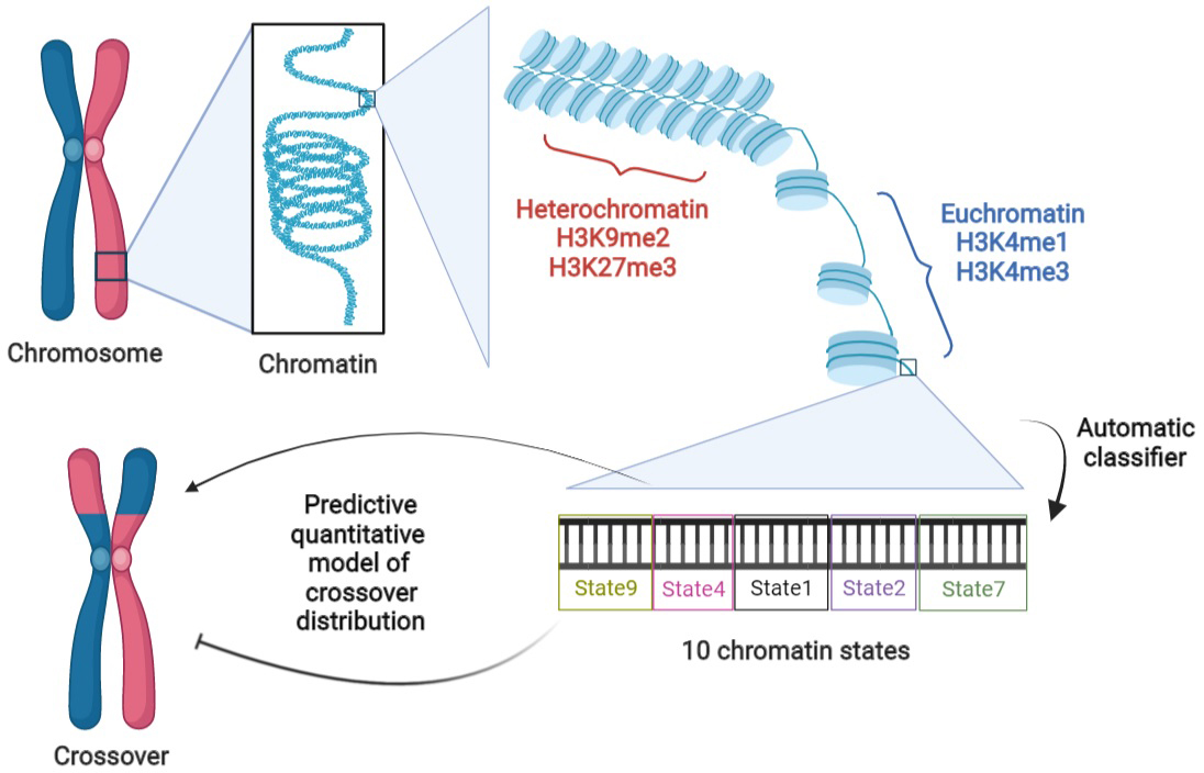
Given the drawbacks of the previous modelling framework, we performed aggregation using an automatic classifier approach (Sequeira-Mendes et al., Reference Sequeira-Mendes, Aragüez, Peiró, Mendez-Giraldez, Zhang, Jacobsen, Bastolla and Gutierrez2014), assigning a ‘chromatin state’ to a local region according to a (non-linear) combination of such features. The methodology is general but those authors implemented it in the case of Col-0, producing 9 chromatin states based on the combination of 16 genomic or epigenomic features, namely H3K4me1, H3K4me2, H3K4me3, H3K9me2, H3K27me1, H3K27me3, H2Bub, H3K36me3, H3K9ac, H3K14ac, H4K5ac, CG methylation, H3 content, H2A.Z, H3.1 and H3.3. Their states 8 and 9 correspond to AT-rich and GC-rich heterochromatic regions, respectively, with state 9 being strongly enriched in the pericentromeric regions. Their seven other states are typically euchromatic. They found that state 1 (respectively state 6) typically colocalises with transcription start sites (TSS) [respectively, transcription termination sites (TTS)]. States 3 and 7 are the most abundant states in gene bodies, with the former one tending to be present with state 1 at the 5′ end of genic regions and the latter one arising more frequently in larger transcriptional units. States 2 and 4 typically lie within intergenic regions and they tend to be proximal and distal to the gene’s promoter, respectively. Like states 2 and 4, state 5 is generally within intergenic regions, but it also arises frequently in silenced genes with high levels of H3K27me3. See also top of Figure 2 for a graphical representation of these trends.

Figure 2. Relations between our 10 chromatin states, genes, intergenic regions and recombination rate. (a) The top pie chart shows the genome-wide occupation percentages of each of the 10 states. ‘SV’ refers to low synteny regions or structural variations between Col-0 and Ler. The characteristics of the nine other states are: state 1 (intragenic, transcription starting site (TSS)), state 2 (intergenic, proximal promoter), state 3 (intragenic, coding sequence), state 4 (intergenic, distal promoter), state 5 (intergenic, H3K27me3 rich), state 6 (intergenic, transcription termination site (TTS)), state 7 (intragenic, long genes), state 8 (heterochromatic, AT rich) and state 9 (heterochromatic, GC rich). The lower pie chart shows the percentage of crossover occurrences identified in the 10 states. (b) Two plots, giving respectively the profiles of cumulated fractions of occurrences of the 10 different states (top) and the recombination rate pattern (bottom) in cM per Mb, along gene bodies and their 3-kb flanking regions. In the absence of SV, the entire 3-kb flanking region was used, otherwise it was truncated. The gene body goes from the TSS to the TTS as given in TAIR 10. Only non-transposable element coding genes satisfying the synteny filter have been included in the analysis. For the gene body region, the x-axis represents relative position, that is the distance from the TSS divided by the distance between TTS and TSS. That procedure allows one to pool genes of different sizes. For the flanking regions, x-axis represents position relative to the TSS or TTS in kb. The blue curve at the bottom is the predicted recombination rate when using the chromatin state profiles at the top together with the genome-wide recombination rates derived from (a). (c) Two plots as in (b) but now for the intergenic regions. Again, the blue curve is the predicted recombination rate when using the chromatin state profiles at the top together with the genome-wide recombination rates derived from (a). The legend in the middle of (b) and (c) indicates the corresponding chromatin state of each color used in plotting the chromatin-state profiles.
Because COs form between homologs, we also need to aggregate information about the local synteny between Col-0 and Ler, the two parents of the F2 population (Rowan et al., Reference Rowan, Heavens, Feuerborn, Tock, Henderson and Weigel2019) used to estimate the recombination landscape. We thus assign the state ‘SV’ to the non-syntenic regions. We then have a total of 10 different ‘states’ that we will study in the rest of this work, referring to them as ‘chromatin states’ even if that is not completely correct. The fraction of the genome covered by any of these chromatin states varies between 5.8 and 13.6%, with state 4 (intergenic, distal) being the most represented and state 8 (heterochromatic, AT rich) the least (cf. Figure 2a, top).
To transform the trends found by Sequeira-Mendes et al. (Reference Sequeira-Mendes, Aragüez, Peiró, Mendez-Giraldez, Zhang, Jacobsen, Bastolla and Gutierrez2014) into quantitative patterns, we have generated the frequency profiles for each chromatin state as a function of position within gene bodies and their flanking regions. For that task, we used the 25,708 genes extracted from syntenic regions and also considered their extensions on both sides, going out to 3 kb upstream of the TSS and downstream of the TTS. The computed profiles (Figure 2b, top) reveal that there is a clear gradient in the chromatin state content along the gene bodies and also along their flanking regions. For instance, the frequency of state 1 has a very sharp rise as one enters the gene on the 5′ side while the frequency of state 7 has a steep fall as one exits the gene on the 3′ side. We performed the analogous computations for intergenic regions and find that the frequency profiles there (cf. Figure 2c, top) have much less variation than in gene bodies.
3.3. A simple quantitative model of recombination rate based on discrete chromatin states and SVs
In contrast to the quantitative variables used in equation (1), the state classifier approach identifies discrete states. These can be used as factors (qualitative variables) in a model of recombination rate by making the perhaps simplistic assumption that each state has its own specific recombination rate. This framework both allows for a direct biological interpretation and is mathematically particularly simple. Comparing the genomic fraction of each chromatin state to the observed CO fraction for that state (top and bottom of Figure 2a) determines the 10 average recombination rates: 3.08, 4.78, 2.16, 6.37, 5.14, 3.48, 1.5, 3.35, 0.7 and 0.57 cM/Mb. Hereafter, these values are referred to as the ‘experimentally measured state-specific recombination rates’. They are to be compared to the genome-wide average recombination rate of 3.3 cM/Mb. As expected, recombination is strongly suppressed in states 9 (pericentromeric heterochromatin) and SV.
In Supplementary Figure S2, we compare experimental recombination rates to those predicted by this minimal ‘model’. For instance, when segmenting the genome into bins of size 100 kb, the fraction of the variance in the experimental recombination rates that is explained by the model is R 2 = 0.24. This value is lower than that of the additive model using equation (1) (cf. Supplementary Table S2) but note that when using the experimentally measured state-specific recombination rates there are no adjustable parameters. Furthermore, this ‘model’ based on chromatin states overcomes the defect of predicting negative recombination rates when gene density is high.
3.4. The model with discrete chromatin states predicts fine-scale recombination patterns
Figure 2b (bottom) shows the recombination rate pattern along genes and their 3-kb flanking regions (same syntenic genes and binning methodology as for the top of that figure). Regions just upstream of the TSS are richer in COs than regions downstream of the TTS which themselves are richer than gene bodies. Interestingly, these recombination patterns are quite well-predicted by the proportions of each chromatin state (top of Figure 2b) using the experimentally measured state-specific recombination rates as displayed by the continuous blue curve in Figure 2b (bottom). This implies that the determinants of recombination rate are at least partly encoded into our 10 states.
We performed the analogous analysis on intergenic regions as shown in Figure 2c (bottom). Again, the experimental behaviour is well-predicted by our model that assigns one recombination rate to each chromatin state (cf. blue curve).

Figure 3. The relationship between the size of intergenic regions and their average recombination rate. These bar charts were constructed using all intergenic regions, but in the bottom, the regions were divided into three categories according to the transcription orientations of the two flanking genes, corresponding to convergent, divergent and parallel transcriptions. In all cases, the x-axis gives the size of the intergenic regions in kb, and the y-axis gives the corresponding averaged recombination rate (cM/Mb). Binning of the intergenic region sizes was applied every 500 bases up to a total size of 10 kb. For example, the leftmost bin covers intergenic regions of size 0–0.5 kb. However, we also include a rightmost bar on each chart to cover intergenic regions of sizes larger than 10 kb. Error bars are errors on the mean computed by the jackknife method (only the top segments are displayed). In both top and bottom figures, the blue curves give the predicted recombination rates using the genome-wide recombination rates of the 10 chromatin states as obtained from Figure 2a. The red curves show the predicted recombination rates when one includes the modulation based on the size of the intergenic regions as specified in equation (4).
3.5. Recombination rate is suppressed in small intergenic regions
The profiles and patterns in Figure 2b,c pool gene bodies or intergenic regions, ignoring their sizes. To further test the model, we have considered the possibility that recombination rate patterns might vary as a function of the size of the region. For instance, the content in exons and introns is quite different for small and large genes and so this could potentially affect recombination rates.
To study the possible influence of gene body size, we divided the genes into size quantiles and recalculated the corresponding state occurrence profiles and recombination rate patterns. As illustrated in Supplementary Figure S3, gene body size strongly affects chromatin state content. Furthermore, recombination rate patterns become more contrasted as gene size increases, with a concomitant decrease in the average recombination rate. Nevertheless, the model of 10 chromatin states correctly predicts these trends as shown by the blue curves.
The analogous study for intergenic region size is summarised in Supplementary Figures S4–S6, treating separately the three possible orientations of the genes flanking the intergenic region: divergent, convergent and parallel. In contrast to the gene body case, the 10 chromatin state models’ predictions (blue curves) are not so good: the model significantly over-estimates the recombination rates when the size of the intergenic region is small.
To quantify this result, consider how the average recombination rate within intergenic regions depends on region size. In Figure 3, we display this dependence, for all intergenic regions pooled (top) or separated according to the orientation of their flanking genes (bottom). There is a clear suppression of recombination rate when the size of the intergenic regions is less than 1.5 kb, while beyond 2.5 kb the curves are rather flat, with perhaps a trend to decrease beyond 10 kb. Figure 3 also displays the recombination rates predicted when using the 10 states chromatin models. Clearly, the predictions over-estimate the recombination rate when the size of intergenic regions is small, in agreement with the trends seen in Supplementary Figure S4–S6.

Figure 4. The relationship between recombination rate and single nucleotide polymorphism (SNP) density. The Col-0 genome was decomposed into bins of 100 kb. For each cross starting with that of Rowan et al. (Reference Rowan, Heavens, Feuerborn, Tock, Henderson and Weigel2019), SNPs and crossovers (COs) were inferred from reads produced using the F2 populations by mapping to the Col-0 genome. SNP density and recombination rates were then determined for each bin and displayed as a scatter plot. The five additional crosses are from Blackwell et al. (Reference Blackwell, Dluzewska, Szymanska-Lejman, Desjardins, Tock, Kbiri, Lambing, Lawrence, Bieluszewski, Rowan, Higgins, Ziolkowski and Henderson2020). The continuous red curves are fits when using the function (a + b x) exp(−cx) so as to maximise the log likelihood. To filter out the high SNP density regions that are expected to causally repress recombination, we restricted the analysis to SNP densities in the first two quantiles. All crosses show a reduced recombination rate at low SNP density and the likelihood ratio test allows us to reject the hypothesis H0 that ‘b = 0’, corresponding to no such suppressive effect (p-values shown for each cross and computed using the chi-square distribution with one degree of freedom).
These results motivated us to improve the model by including a modulation effect taking into account the sizes of intergenic regions. We parameterise this modulation by multiplying the recombination rate ri of a segment in state i by the factor

whenever the segment lies within an intergenic region of size ℓ kb. The detailed form of this modulation function is not so important, but it should go smoothly from its minimum at ℓ = 0 to its maximum at large ℓ. The quantities ${\beta}_1$
,
${\beta}_1$
, ${\beta}_2$
and
${\beta}_2$
and ${\beta}_3$
are free parameters that we can adjust to minimise the deviation between observed and predicted recombination rates over all intergenic regions. The red curves in Figure 3 show the corresponding improved predictions when including this modulation effect.
${\beta}_3$
are free parameters that we can adjust to minimise the deviation between observed and predicted recombination rates over all intergenic regions. The red curves in Figure 3 show the corresponding improved predictions when including this modulation effect.
3.6. Recombination rate is suppressed in regions of low SNP density
A high divergence between homologs suppresses recombination rate, a trend that is visible in the top left of Figure 4, where SNP density is used as a proxy for divergence between homologs. However, we see that low SNP density is also associated with reduced recombination. To confirm that this is not an artefact of the Rowan et al. (Reference Rowan, Heavens, Feuerborn, Tock, Henderson and Weigel2019) dataset, we examined five other crosses published by Blackwell et al. (Reference Blackwell, Dluzewska, Szymanska-Lejman, Desjardins, Tock, Kbiri, Lambing, Lawrence, Bieluszewski, Rowan, Higgins, Ziolkowski and Henderson2020) who had found the same effect. The minor differences between our panels and those in their paper come from using different choices in the analysis pipelines: including or not the pericentromeric regions, using a bin size of 100 kb versus 1 Mb, applying different filtering criteria to the remapped reads to define SNPs, and forbidding or not the fitting function to have negative values. The important point is that the two independent analyses reach the same conclusion: low SNP density is associated with lower recombination rate (cf. Figure 4).
3.7. Low SNP density may be a causal factor of recombination rate suppression
In natural populations undergoing panmictic reproduction and subject to spontaneous mutations, drift generates linkage disequilibrium depending on recombination rate. Indeed, if a region of the genome has lower than average recombination rate, it will sustain larger haplotypic blocs and so its SNP density will be below average, producing the kind of correlation found in Figure 4. However, A. thaliana is a selfer, so linkage disequilibrium and thus the pattern of accumulation of mutations will not be affected by recombination. Specifically, if we consider the most recent common ancestor to Col-0 and Ler, it produced two separate lineages by successive generations of selfings, lineages in which mutations have accumulated independently. Under such dynamics, recombination cannot influence SNP density unless recombination itself generates mutations. This last possibility has long been downplayed because homologous recombination was considered to be nearly error-free (Guirouilh-Barbat et al., Reference Guirouilh-Barbat, Lambert, Bertrand and Lopez2014), but it is now known that CO formation produces mutations in human (Arbeithuber et al., Reference Arbeithuber, Betancourt, Ebner and Tiemann-Boege2015; Halldorsson et al., Reference Halldorsson, Palsson, Stefansson, Jonsson, Hardarson, Eggertsson, Gunnarsson, Oddsson, Halldorsson, Zink, Gudjonsson, Frigge, Thorleifsson, Sigurdsson, Stacey, Sulem, Masson, Helgason, Gudbjartsson and Stefansson2019). In the absence of any such evidence in plants, we formalised as follows a test for the possibility that SNP density influences recombination. We fit each scatter plot of Figure 4 to the function (a + b x) exp(−cx) that embodies a suppression effect at low SNP density. Then we compare the likelihood for that fit to the one obtained when the parameter b is set to 0 (corresponding to no suppression at low SNP density). The likelihood ratio test then allows us to reject or not the absence of this suppression effect. In all six populations, the p-value shows that the data strongly favours the presence of a suppression. A slightly modified formalisation is tested in the Supplementary Material (cf. Figure S7), reaching the same conclusion.
3.8. A state-based quantitative model with multiple effects modulating recombination rate has good predictive power
Our quantitative model builds on the framework of 10 discrete chromatin states by assigning to each an adjustable base recombination rate, but also by applying three context-dependent multiplicative modulating effects. The first effect is associated with intergenic region size ℓ: we parameterise the multiplicative modulation via the function 1/( ${\beta}_1$
+
${\beta}_1$
+ ${\beta}_2$
exp(−
${\beta}_2$
exp(− ${\beta}_3$
ℓ)), where ℓ is the size of the intergenic region in kb. The second effect is associated with SNP density ρ: we multiply the recombination rate by (1 +
${\beta}_3$
ℓ)), where ℓ is the size of the intergenic region in kb. The second effect is associated with SNP density ρ: we multiply the recombination rate by (1 + ${\alpha}_1$
ρ) exp(−
${\alpha}_1$
ρ) exp(− ${\alpha}_2$
ρ). Lastly, at the whole chromosome level, it is known that CO numbers are tightly regulated with the result that genetic lengths do not vary linearly with genome size, especially in species that have chromosomes of very different physical lengths. This regulation presumably arises through both CO ‘interference’ (COs tend to be well separated) and the obligatory CO (there is at least one CO per bivalent), both of these acting on large rather than fine scales. As a result, the recombination rate of a specific genomic segment can be significantly higher if it belongs to a small chromosome than if it belongs to a large one. To incorporate this chromosome-wide effect, we rescale all predicted recombination rates within a chromosome to enforce its experimentally measured genetic length.
${\alpha}_2$
ρ). Lastly, at the whole chromosome level, it is known that CO numbers are tightly regulated with the result that genetic lengths do not vary linearly with genome size, especially in species that have chromosomes of very different physical lengths. This regulation presumably arises through both CO ‘interference’ (COs tend to be well separated) and the obligatory CO (there is at least one CO per bivalent), both of these acting on large rather than fine scales. As a result, the recombination rate of a specific genomic segment can be significantly higher if it belongs to a small chromosome than if it belongs to a large one. To incorporate this chromosome-wide effect, we rescale all predicted recombination rates within a chromosome to enforce its experimentally measured genetic length.
Overall our model has 15 adjustable parameters: the 10 base recombination rates and the 5 additional parameters for the modulation effects (the chromosome-specific rescalings do not require introducing any parameters or fits). To calibrate the resulting quantitative model, we apply the maximum likelihood approach which quantifies the deviation between the model’s predicted rates and the experimental ones from Rowan et al. (Reference Rowan, Heavens, Feuerborn, Tock, Henderson and Weigel2019) when using a binning along the genome (see Section 2 for details). In Supplementary Table S3, we provide the AIC and BIC values when the additional parameters are successively included. The minimum value is always reached for the full (highest complexity) model which is why we discuss only that case hereafter. The optimised parameters are provided in Supplementary Table S4 when calibrating over the whole genome using various bin sizes. In Supplementary Figure S8, we compare the predictions of recombination rate in our quantitative model to the experimental ones when using bins sizes ranging from 50 to 500 kb. One can also do the comparison at the level of the recombination landscapes: in Figure 5, we show the predicted and experimental landscapes for chromosome 1 when using bins of size 100 kb (cf. Supplementary Figure S9 for the other chromosomes). We see that the adjusted model reproduces much of the qualitative structure of the landscape. The inset in Figure 5 provides a zoom on a region in the right arm, allowing one to better see the small scale trends. Even for this bin size which is rather large compared to the typical distance between genes, the model and experimental landscapes are far from smooth. Furthermore, both in the inset and in the main part of the figure, we see that though there is quite a lot of concordance between the two curves for local minima and maxima, the model’s landscape generally underestimates the observed variance. This is partly due to the experimental landscape being subject to the stochasticity of CO numbers, but it may also point to other determinants that could be missing in our analysis or data.

Figure 5. Experimental and predicted recombination landscapes of chromosome 1. Landscapes using 100 kb bins obtained from the Rowan et al. (Reference Rowan, Heavens, Feuerborn, Tock, Henderson and Weigel2019) dataset (red) and predicted from our calibrated model based on chromatin states (blue) with 15 parameters. Inset: a zoom in the right arm. For landscapes of all chromosomes, see Supplementary Figure S9.
Finally, to test the predictive power of our modelling approach and ensure that it does not introduce overfitting, we also have calibrated the model on one chromosome and then used that calibration to predict recombination on the other chromosomes. Supplementary Table S5 gives the corresponding values of R². For comparison, we perform the same test in Supplementary Tables S6 and S7 when using the additive model (equation (1)) or its extension with interactions (equation (3)). Clearly, our model has significantly higher predictive power than those other models.
4. Discussion and conclusions
4.1. Aggregated chromatin states as predictors of recombination rate
The genome-wide distribution of COs is expected to follow largely from the degree to which the double strand break machinery can access the DNA. This will depend of course on the state of the chromatin and indeed many genomic and epigenomic features are empirically found to correlate with recombination rate. Qualitative modelling based on such features allows one to distinguish hot versus low recombination regions (Demirci et al., Reference Demirci, Peters, de Ridder and van Dijk2018) but quantitative modelling has been limited to frameworks like equations (1) and (3) (Blackwell et al., Reference Blackwell, Dluzewska, Szymanska-Lejman, Desjardins, Tock, Kbiri, Lambing, Lawrence, Bieluszewski, Rowan, Higgins, Ziolkowski and Henderson2020; Rodgers-Melnick et al., Reference Rodgers-Melnick, Bradbury, Elshire, Glaubitz, Acharya, Mitchell, Li, Li and Buckler2015). Unfortunately, the dependence on a feature is typically non-monotonic as displayed in Figure 1. As a result, recombination rate modelling using these features as quantitative variables requires strong non-linearities and leads to an unmanageable combinatorial complexity (cf. the 46 parameters in equation (3)), not to mention problems for interpreting the resulting models and their low prediction power (cf. Supplementary Tables S6 and S7). To overcome this difficulty, we use a classifier approach to automatically aggregate 16 genomic and epigenomic features into discrete classes (Sequeira-Mendes et al., Reference Sequeira-Mendes, Aragüez, Peiró, Mendez-Giraldez, Zhang, Jacobsen, Bastolla and Gutierrez2014). This defines the starting point of our modelling wherein each position of the genome is considered to be in one of 10 chromatin states. Using the genome-wide recombination rates in each of these 10 states, Figure 2b,c shows that recombination patterns around genes and in intergenic regions are rather well predicted. In particular, near the extremities of genes, this simple modelling leads to enhanced recombination rates, in agreement with experiment (Choi et al., Reference Choi, Zhao, Kelly, Venn, Higgins, Yelina, Hardcastle, Ziolkowski, Copenhaver, Franklin, McVean and Henderson2013; Kianian et al., Reference Kianian, Wang, Simons, Ghavami, He, Dukowic-Schulze, Sundararajan, Sun, Pillardy, Mudge, Chen, Kianian and Pawlowski2018; Marand et al., Reference Marand, Jansky, Zhao, Leisner, Zhu, Zeng, Crisovan, Newton, Hamernik, Veilleux, Buell and Jiang2017).
4.2. Intergenic region size modulates recombination rate
The simple model using genome-wide recombination rates in each of the 10 states does not adequately predict the suppressed recombination rate in small intergenic regions (cf. Figure 3). This suppression effect could be the consequence of a local context affecting chromatin accessibility for biophysical reasons. A first such reason could be that small intergenic regions are partly hidden from the double strand break machinery by their flanking regions when these are in dense chromatin. A second such reason could be the way chromatin loops are organised in meiosis; if denser chromatin (e.g., containing gene bodies) is preferentially tethered to the base of those loops, it will pull along with it adjacent stretches of open chromatin, hiding these from the double strand break machinery (Tock & Henderson, Reference Tock and Henderson2018).
4.3. Lack of any sequence divergence may drive lower recombination rate
The empirical data in multiple crosses show that regions with very low divergence between homologs typically have low recombination rate (cf. Figure 4). That is expected in panmictic populations where recombination shapes linkage disequilibrium and thus SNP density. However, A. thaliana is a selfing species with a very low rate of outcrossing of about 2% (Hoffmann et al., Reference Hoffmann, Bremer, Schneider, Burger, Stolle and Moritz2003; Platt et al., Reference Platt, Horton, Huang, Li, Anastasio, Mulyati, Ågren, Bossdorf, Byers, Donohue, Dunning, Holub, Hudson, Le Corre, Loudet, Roux, Warthmann, Weigel, Rivero and Borevitz2010). That leads to low genetic divergence within given habitats which is further exacerbated by adaptive pressures, so recombination in the wild will hardly do any allelic shuffling. We thus argue that our observations from the data in this species might be explained if an absence of divergence between homologs causally suppresses COs. Clearly, such an effect makes sense from an evolutionary perspective: if a genomic region has no underlying sequence diversity, there is little point in producing COs there.
Interestingly, a reduction of recombination rate caused by near perfect sequence homology was demonstrated in three previous works on A. thaliana. The oldest such work, by Barth et al. (Reference Barth, Melchinger, Devezi-Savula and Lübberstedt2001), found that on average homozygous homologs led to fewer COs than heterozygous ones. Second, Ziolkowski et al. (Reference Ziolkowski, Berchowitz, Lambing, Yelina, Zhao, Kelly, Choi, Ziolkowska, June, Sanchez-Moran, Franklin, Copenhaver and Henderson2015) considered a heterozygous block within an otherwise homozygous chromosome and found that CO frequency was enhanced in the heterozygous region. Third, Blackwell et al. (Reference Blackwell, Dluzewska, Szymanska-Lejman, Desjardins, Tock, Kbiri, Lambing, Lawrence, Bieluszewski, Rowan, Higgins, Ziolkowski and Henderson2020) showed that msh2, a mutant of mismatch repair, redistributed COs towards regions of lower SNP density, suggesting that, in wild type, CO formation is disadvantaged when sequence homology is perfect. The behaviours found in all these works can be interpreted as a large-scale manifestation of the causal SNP effect we hypothesise.
4.4. A quantitative model of recombination rate with good predictive power
Our full model integrates local genomic and epigenomic features but also context-dependent information. All of its 15 parameters have very direct interpretations and are statistically justified by the AIC and BIC tests (cf. Supplementary Table S3). This model has good predictive power as shown in Supplementary Tables S5–S7 and is able to reproduce much of the variation in rates arising in the recombination landscape (cf. Figure 5 and Supplementary Figure S9). Clearly not all of the variation is captured by our model. First, there is statistical noise inherent to the experimental landscape. Second, although the model predicts major peaks and troughs in the landscape, it tends to underestimate their amplitude. This may suggest a form of competition between sites for recruiting the machinery that produces double strand breaks. There are also other caveats to our modelling. The most obvious one is that because of lack of appropriate data, we had to use measurements of epigenetic marks in Col-0 only and from tissues such as leaf or root rather than from meiocytes. Fortunately, it seems that the epigenetic landscape is largely shared between somatic and germline tissues, the differences being restricted to a small fraction of the genome (Walker et al., Reference Walker, Gao, Zhang, Aldridge, Vickers, Higgins and Feng2018). We did a systematic investigation of this point using published data (cf. Supplementary Figure S1) and showed that the epigenomic patterns are surprisingly similar between somatic and germline tissues. Another limitation of our modelling is that it necessarily ignores any sex-dependent differences in recombination landscapes, focussing only on the female–male average. Similarly, we have not explicitly included CO interference or the obligatory CO, we have just incorporated a proxy of their effects via chromosome-specific rescalings. Such a choice is in line with the expectation that CO interference and the obligatory CO shape recombination landscapes on large scales (Lloyd & Jenczewski, Reference Lloyd and Jenczewski2019; Morgan et al., Reference Morgan, Fozard, Hartley, Henderson, Bomblies and Howard2021), leaving open the determinants at fine scales. Lastly, but perhaps very importantly, we take no account of the well-known fact that meiotic chromosomes are organised in loops tethered to an axis. This structural aspect of meiotic chromosomes may be important for modulating local recombination rates and it is tempting to conjecture that these loops may be responsible for the large peaks seen in the recombination landscape (cf. Figure 5 and Supplementary Figure S9). Unfortunately, very little is known about these loops, in particular concerning their size, position and variability across genetic backgrounds. Hopefully, these uncertainties will be lifted in the near future, given that standard chromosome conformation capture techniques applied to meiotic cells should provide the required information quite directly.
Acknowledgements
We thank T. Blein, M. Rousseau-Gueutin and P. Sourdille for discussions and we are particularly indebted to M. Grelon who provided multiple feedback on our drafts. We are also grateful to B. Rowan and I. Henderson for sharing their data.
Financial support
GQE – Le Moulon and IPS2 benefit from the support of Saclay Plant Sciences-SPS (ANR-17-EUR-0007). The work of Y-M. Hsu was supported by a PhD grant provided by the Ministry of Education (Taiwan) and Université Paris-Sud/Saclay.
Conflicts of interest
The authors declare no potential conflicts of interest.
Authorship contributions
M.F. and O.M. conceived the study. O.M. designed the modelling. Y.M.H. performed all the bioinformatics and code writing necessary for the subsequent analyses. All authors worked on the analyses and wrote the article.
Data availability statement
This work produced no new data but exploited previously published data (see Section 2, Supplementary Material and Supplementary Table S1). All pipelines and analysis codes are given as Supplementary files.
Supplementary Materials
To view supplementary material for this article, please visit http://doi.org/10.1017/qpb.2021.17.


 Open access
Comments
Dear colleagues,
Genetic recombination shuffles alleles between parental chromosomes to generate novel combinations to be passed on to offspring. That shuffling is a cornerstone for research in genetics, it is one of the most important forces in natural evolution and it is key for artificial genetic improvement (e.g. plant breeding). The distribution of meiotic crossovers along chromosomes is strikingly heterogeneous on all scales: large heterochromatic pericentromeric regions are nearly totally devoid of crossovers while hot spots of recombination typically arise in regions of 1 kb or less. Although the qualitative trends of such "recombination landscapes" (repression in heterochromatin, enrichment in intergenic regions) are common to nearly all species studied, there have been hardly any attempts to really model these landscapes. The two fundamental reasons are (i) lack of high quality data and (ii) the fact that many different genomic or epigenomic features are expected to affect recombination rate. To overcome this last difficulty, theoretical investigations of these landscapes have relied on two frameworks. The first is standard quantitative genetics, leading to linear and generalized linear models (allowing for interactions also). The second is supervised learning which is qualitative rather than quantitative (regions are only classified as high vs low in recombination rate, cf. Demirci et al 2018 cited in our manuscript).
In the work presented in this manuscript, we have been able to construct a quantitative model reproducing the recombination landscape of Arabidopsis thaliana, a species chosen because of its available data, both genomic and epigenomic. Rather than use one of the two frameworks mentioned above, we take a third path allowing us to escape the pitfalls of those high complexity models. Notably, (i) our model explains a substantial fraction the variance in recombination rate, (ii) it is predictive while the models based on quantitative genetics are not, (iii) its different parameters all have a direct interpretation, either as base recombination rates or as motivated factors modulating those rates. Given these successes, our work will interest scientists working on recombination rates. But, more generally, our framework is likely to inspire researchers attempting to model complex biological systems driven by a plethora of factors. If we hope to publish in "Quantitative Plant Biology" it is because it has precisely the readers we want to target: readers motivated by quantitative and predictive modeling solidly anchored in plant biology.
Sincerely yours,
Y.-M. Hsu, M. Falque and O. Martin