


Introduction
The occurrence of floods and mudflows during the eruption of Mount St Helens, Washington, USA, and documented large water-saturated mudflows from Mount Rainier and Mount Adams, Washington, indicate the need for ice- thickness measurements to help predict the water hazard of other Cascade Range volcanoes (Reference Driedger and KennardDriedger and Kennard, 1986). The biggest hazards from Mount Baker, Washington (Fig. 1), and Mount Adams (Fig. 2) are not eruptions, but debris avalanches and lahars partially lubricated by ice, snow and meltwater (Reference Gardner, Scott, Miller, Myers, Hildreth and PringleGardner and others, 1995;Reference Scott, Iverson, Vallance and HildrethScott and others, 1995;Reference VallanceVallance, 1999). Other hazards include removal of ice and snow during eruptions which leads to flooding and melting of ice and snow that contributes to phreatic and hydrothermal eruptions (Reference MastinMastin, 1995). However, few ice-thickness measurements have been made directly on these and other Cascade volcanoes (Reference Driedger and KennardDriedger and Kennard, 1986).

Fig. 1. Location map (inset) and aerial photograph for Mount Baker. Red lines indicate profiles shown in Figure 4. Radar data from Reference HarperHarper (1993), Reference Tucker, Driedger, Nereson, Conway and ScurlockTucker and others (2009) and Reference ParkPark (2011).
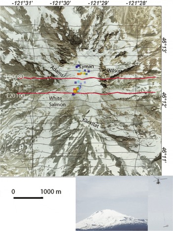
Fig. 2. Aerial photograph of Mount Adams. Red lines indicate profiles shown in Figure 5. Drillhole data are from Reference FowlerFowler (1936) and radar data are from a personal communication from S. Tulaczyk (2006). Ice-thickness scale as for Figure 1. Inset shows photograph of Mount Adams viewed from the southwest with the helicopter and HEM bird.
This paper reports the pioneering use of helicopter electromagnetic (HEM) data, originally collected to detect hydrothermal alteration (Reference Finn, Sisson and Deszcz-PanFinn and others, 2001, Reference Finn, Deszcz-Pan, Anderson and John2007a,Reference Finn, Deszcz-Pan, Horton, Breit and Johnb; Reference Finn and Deszcz-PanFinn and Deszcz-Pan, 2009), to estimate ice thickness for parts of Mount Baker (Fig. 1) and Mount Adams (Fig. 2) and also releases the ice-thickness data (Supplementary Spreadsheets 1 and 2, http://igsoc.org/hyperlink/11j098_supp_ss1.xlsxand http://igsoc.org/hyperlink/11j098_supp_ss2.xlsx). Other HEM studies of ice thickness are restricted to those on sea ice (Reference Kovacs and HolladayKovacs and Holladay, 1990; Reference Pfaffling, Haas and ReidPfaffling and others, 2007; Reference Haas, Lobach, Hendricks, Rabenstein and PfafflingHaas and others, 2009). Other electromagnetic methods in addition to standard ground-penetrating radar (GPR) techniques, such as magnetotelluric and Schlumberger d.c. measurements on polar ice sheets (Reference Shabtaie and BentleyShabtaie and Bentley, 1995;Reference Wannamaker, Stodt, Pellerin, Olsen and HallWannamaker and others, 2004) and temperate glaciers (Reference Rothlisberger and VogtliRothlisberger and Vogtli, 1967), have been successful in delineating ice thickness. We focus on the innovative approach of using resistivity inversions to obtain ice thickness. Comparison of the HEM results with ice- penetrating radar measurements and drillhole data helps to determine their reliability.
Radar and Drillhole Estimations of Ice Thickness on Mount Baker and Mount Adams
Existing radar measurements indicate that Easton Glacier, Mount Baker, ranges in thickness from 30 to 107 m (Reference HarperHarper, 1993; Fig. 1). A 470m long radar profile across Carmelo Crater, Mount Baker, revealed a maximum thickness of ~82 m with measurement uncertainties ~±5 m (Reference Tucker, Driedger, Nereson, Conway and ScurlockTucker and others, 2009; Fig. 1). A recent GPR survey over Sherman Crater revealed a maximum thickness ranging from ~58 to 71 m, depending on summer melt rates (Reference Park, Clark, Caplan-Auerbach, Larsell, Hogan and BushPark and others, 2009;Reference ParkPark, 2011). Previously the volume of glacier ice on Mount Baker was estimated from statistical analysis of characteristics for all measured glaciers based on topographic maps and aerial photographs, and determined to be ~-1800 × 106m3 (Reference KennardKennard, 1983;Reference Driedger and KennardDriedger and Kennard, 1986).
On Mount Adams, holes drilled into the summit ice cap in the 1930s as part of a sulfur mining operation (Reference FowlerFowler, 1936) can be used for crude estimates of ice thickness (Fig. 2). In addition, 700 m of new GPR data along five survey lines were collected on the southwestern portion of Mount Adams (Fig. 2) in July 2006 using a portable pulseEKKO 100 radar system with a 1000V transmitter and 100 MHz antennas. The basal reflector was well defined at shallow depths (~0–30m) but became increasingly diffuse deeper down such that the resolution of its position decreased. The ice thickness reached nearly ~120m in the southwest portion of the Mount Adams summit ice cap (personal communication from S. Tulaczyk, 2006).
Temporal changes in the thickness of the ice between the HEM- and the radar- and drillhole-determined ice thickness are likely. For example, the change in mass balance of Easton Glacier between the 1991 radar survey there (Reference HarperHarper, 1993) and the 2002 HEM survey resulted in a <5 m (Reference PeltoPelto, 2008) to 6.7 m change in thickness (Reference Granshaw and FountainGranshaw and Fountain, 2006), within the errors of the radar and HEM measurements. However changes in snow thickness up to ~15 m in 1 year have been observed at Mount Baker (Reference ParkPark, 2011). The May 2002 dates of the HEM surveys are near the April snowpack maxima at a variety of weather sites in Washington (Reference PeltoPelto, 2008), whereas the drillhole and radar surveys were taken late in the summer (Reference HarperHarper, 1993; personal communication from S. Tulaczyk, 2006;Reference Tucker, Driedger, Nereson, Conway and ScurlockTucker and others, 2009;Reference ParkPark, 2011) during snowpack minima. In addition, the aerial photographs used in this paper (Figs 1, 2 and 4–7) were taken in late July 2010 when the snow levels can be as much as 10m lower than the May 2002 time frame for the surveys (Fig. 2 inset). Finally, the drillhole and radar data indicate that ice thickness can change significantly (tens of meters) over short distances (Figs 1 and 2). Despite the spatial and temporal variability and uncertainties in old ice-thickness measurements, particularly in the locations of the drillholes, these data can be used to help validate the HEM-derived ice-thickness estimates.
Hem VS Radar Electromagnetic Response
The electrical properties of the Earth dictate the response characteristics of all electromagnetic systems:
where k is the wavenumber, u is the angular frequency, a is the ground conductivity, n is the magnetic permeability and e is dielectric permittivity. For HEM systems, the diffusion term ( ωσμ is generally much larger than the propagation term ( ω 2 σμ). For typical radar systems, the opposite is true because of significantly higher (MHz-GHz) frequencies measured by radar compared with the HEM system (400 Hz-100 kHz).
In HEM systems, a transmitter in the bird emits electromagnetic energy at several discrete frequencies, which induces currents in conductive ground below resistive ice. The induced currents generate small in-phase and quadrature components of magnetic fields that are measured, in parts per million of the transmitted signal, by the system receiver (in the bird) with a precision of ~1 ppm. The strength of the currents is proportional to the conductivity of the ground and the frequency and power of the transmitting coil, and rapidly decreases with increasing distance between the transmitter and the ground. Thickening of the ice increases the distance between the transmitter and the ground, resulting in weakening of eddy currents below the ice. The attenuation of all electromagnetic waves is proportional to the product of the conductivity of the ground and frequency of the system. Because HEM systems use much lower frequencies than radar, their penetration in conductive ground exceeds that of the penetration of a few meters of the higher-frequency radar systems. The penetration depth depends on the transmitter frequency. For resistive ground (ice) the HEM and radar signals are not strongly attenuated. This allows the radar signal, which consists of pulses of electromagnetic waves, to travel great distances (thousands of meters) until they are reflected from conductive interfaces such as the base of the ice. In the same area, the HEM signal passes through the resistor unattenuated until it reaches the conductor where it generates eddy currents. If the basement is conductive and within ~100m of the surface, the HEM system measures a strong signal. On the other hand, if the basement is resistive, the generated eddy currents are weak and the HEM system fails to measure their response.
Helicopter Electromagnetic Surveys
Helicopter-borne electromagnetic and magnetic data were collected in May 2002 every ~3.5m along east-west trending lines spaced 250 m apart (Figs 1 and 2a) (personal communication from Fugro Survey Ltd, 2002). The multifrequency HEM Resolve system consisted of five coplanar and one coaxial transmitter and receiver coils carried in a bird (Fig. 2 inset). The system transmitted electromagnetic energy at six frequencies (106 400, 25 400, 6121, 1515 and 388 Hz for coplanar and 3315 Hz for coaxial coils). Coplanar coils were separated by 7.9m;coaxial coil separation was 9 m. Locations of the bird were determined through high- accuracy differential GPS (1 m) and a laser altimeter with sub-meter accuracy mounted on the bird. In addition, a radar altimeter (1 m accuracy) was mounted in the helicopter (personal communication from Fugro Survey Ltd, 2002). Comparison of the GPS, radar and laser altimeter data showed that the laser obtained the best elevations overall, as in other HEM surveys (Reference Fitterman and YinFitterman and Yin, 2004;Reference Davis, Macnae and HodgesDavis and others, 2009). Although the laser data were not corrected for roll of the bird, video footage indicates minimal swinging of the bird in normal flight conditions. The most severe swinging occurred during the helicopter ascent, where densely sampled data (because of the slow helicopter speed) partly compensated for the increased swinging. A good indication of the accuracy of the laser elevations is to compare them with the radar data corrected for the length of the bird cable and GPS data with the 10m digital elevation model (DEM) subtracted. All altitude data match to within ~1–2m over flat regions (e.g. the summit and edges of Mount Adams, Carmelo and Sherman Craters and edges of Mount Baker), indicating good elevation control (Reference Fitterman and YinFitterman and Yin, 2004). Over the steep slopes, the laser elevations exceed the radar by as much as 25 m. The radar senses the slope adjacent to the bird, resulting in elevations that are too small relative to the laser, which more accurately measures the distance of the bird to the ground directly beneath it, as found in other regions such as Nebraska (Deszcz-Pan, unpublished data). Although it is difficult to determine the exact elevation error for these regions, our elevation comparisons suggest the resolution of the laser is generally <5 m.
The HEM system responds to variations in system elevation above conductors that correspond to the flattest areas on the volcanoes where the elevation control is tightest. This response is highest for small elevation changes above the conductor and decreases with increasing distance to the conductor. If the conductor corresponds to the basement beneath the ice, the HEM system can detect this boundary (within certain limitations), but might not be able to resolve the thickness and resistivity of the overlying resistive layer (ice) if the system elevation is not well known. In the resistive areas, where the signal is low, the contrasts between the air and resistive ground are smaller and frequently the system elevation and resistivity and thickness of the top layer are not well resolved.
The HEM system averaged 53 m above the surface for Mount Baker (Fig. 1) and 82 m for Mount Adams (Fig. 2). If the HEM sensor elevation is too high, the signal level diminishes and the system response drops below noise levels. To test whether the quality of the data collected over the volcanoes was significantly compromised by high survey elevations, we calculated absolute noise values (ppm) following a standard HEM noise model (Tolboll and Christensen, 2006).
If the ground is resistive, its effect on the measurements at high elevations is minimal and the HEM system measures the system noise. In the Mount Baker and Mount Adams surveys, high bird elevations exceeding 150 m are restricted to the resistive flanks of the volcanoes. The data collected in these areas represent the system noise used to estimate the absolute noise of both the Mount Baker (Table 1) and Mount Adams surveys (Table 2).
Table 1. Mount Baker survey absolute standard noise

Table 2. Mount Adams survey absolute standard noise
The total absolute noise level N total abs of the individual measurements is the sum of an absolute stochastic noise contribution N stoc abs and a contribution for inadequate drift corrections Ndrift abs (Tolboll and Christensen, 2006). Nstoc abs is estimated by calculating the peak-to-peak noise (3 SD) of the signal measured at high elevations, where the effect of the ground is minimal and the HEM system measures mostly the system noise. The highest (>150 m) system elevations were over the resistive flanks of the volcanoes, and the data collected in these areas were used to estimate the absolute stochastic noise of both the Mount Baker (Table 1) and Mount Adams surveys (Table 2). On Mount Baker (Table 1) there were about 1500 points (out of a total of 100 300) and on Mount Adams (Table 2) there were 6200 points (out of a total of 86 752) recorded above the 150 m bird elevation.
The other component of the standard noise model is the contribution from nonlinear system drift. In standard data processing, the drift is assumed to be linear and is removed from the data by linear interpolation of differences in highaltitude (>400 m elevation) measurements. To estimate the nonlinear component of the drift we recalculated the drift thatwas removed from final data by extracting unleveled data collected above 400 m elevation (from the turns between lines) and calculating the differences between them. Fifteen percent of the averaged high-altitude differences were added to the stochastic noise to account for the nonlinearity of drift (Tables 1 and 2), a standard but somewhat arbitrary correction (Tolboll and Christensen, 2006). Other sources of errors can significantly exceed the stochastic noise, such as calibration errors, non-one-dimensional geology, topography, and variations in system geometry (Reference SiemonSiemon, 2009). These relative effects are typically 5% of the measured values (Tolboll and Christensen, 2006). This 5% relative value was confirmed by an independent analysis of errors for selected areas on Mount Baker and Mount Adams estimated by a stochastic process (Reference MinsleyMinsley, 2011). For every point in the inversion, we used the larger of the absolute noise (N total abs) or 5% of the measured data in order to obtain the most conservative noise model, recognizing that drift and calibration errors will not be precisely represented.
Modeling of HEM Data
The HEM system is designed to detect low-resistivity rocks within the upper 100–200 m of the surface. Previous resistivity inversion modeling constrained with rock and ice physical properties, magnetic models and geologic mapping at Mount Baker (Reference Finn and Deszcz-PanFinn and Deszcz-Pan, 2009) and Mount Adams (Reference Finn, Deszcz-Pan, Anderson and JohnFinn and others, 2007a) was aimed at locating low- resistivity altered volcanic rocks that might source large debris avalanches. The models identify surface layers of highly resistive ice (>10 000 Ωm) underlain by basement with resistivities that vary depending on degree of alteration and water saturation. The resistivities of wet altered rocks found under Sherman Crater and Dorr Fumarole fields at Mount Baker (Reference Finn and Deszcz-PanFinn and Deszcz-Pan, 2009) and the summit at Mount Adams (Reference Finn, Deszcz-Pan, Anderson and JohnFinn and others, 2007a) are <100 Ωm and typically <10fim, whereas wet fresh volcanic rocks have resistivities >~100 Ωm but <~850 Ωm. Once the basement resistivities exceed ~1000 Ωm, as for dry massive volcanic rocks, their actual resistivities are not well resolved in the models (Reference Finn, Deszcz-Pan, Anderson and JohnFinn and others, 2007a,b) and so cannot be differentiated from ice. In order to locate the ice-rock interface, we applied several approaches: smooth Occam- type resistivity inversion (Reference Farquharson, Oldenburg and RouthFarquharson and others, 2003) and least-squares (Reference AndersonAnderson, 1982) and laterally constrained (Reference Auken, Christiansen, Jacobsen, Foged and SorensenAuken and others, 2005) two-layer inversions.
One-dimensional (1-D) forward modeling
To evaluate the reliability of determining ice thickness from the HEM data, we calculate expected ranges of ice-thickness values obtained from inversion of theoretical data for a specific HEM system of six frequencies and survey parameters (noise (Mount Baker (Table 1) and Mount Adams (Table 2)) and fixed 50 m elevation) and specified basement resistivities appropriate for local geologic conditions (Reference Auken, Nebel, Sorensen, Breiner, Pellerin and ChristensenAuken and others, 2002). The resistivity model approximates the local conditions and contains variably thick (0–125 m) resistive (10 000 Ωm) ice over basement with variable resistivities. Data uncertainty (factor SD) for each model and frequency is calculated as the amplitude of the ratio of standard noise/(forward model response × 100) (Reference Auken, Nebel, Sorensen, Breiner, Pellerin and ChristensenAuken and others, 2002).
If the resistivity of the basement is low (e.g. <100 Ωm), the calculated ice thickness closely approximates the true layer thickness for depths <60 m, is within ~10m for ice thickness between 60 and ~90m and exceeds 25 m for ice thickness >100 m (Fig. 3). For 300 Ωm basement resistivity, the uncertainty in ice-thickness estimate exceeds 25 m for 75 m thick ice and is ~5m for ice <~50m thick (Fig. 3). For basement resistivities between 300 and ~850 Ωm, ice thickness <~35 m can be determined reliably. For thin ice (<~10m) and resistive basement (300–850 Ωm) the ice thickness is not resolved because there is not enough difference in response between them.

Fig. 3. Uncertainties in ice-thickness estimates as a function of ice thickness and basement resistivity. The x-axis represents the true layer thickness and the y-axis represents the maximum and minimum thickness of ice estimated from the inversion of data at six frequencies, assuming a given noise (Reference Auken, Nebel, Sorensen, Breiner, Pellerin and ChristensenAuken and others, 2002). Color-coded lines represent the expected range of thickness estimates depending on the basement resistivity compared with the true ice thickness. The curves are truncated where ice-thickness resolution is low, chosen to be twice the true ice-thickness value.
1-D inversion
We invert the data for the ice thickness using 1-D inversions to produce smooth, Occam-type resistivity sections (Reference Farquharson, Oldenburg and RouthFarqu-harson and others, 2003) and least-squares (Reference AndersonAnderson, 1982) and laterally constrained (Reference Auken, Christiansen, Jacobsen, Foged and SorensenAuken and others, 2005;Reference SiemonSiemon and others, 2009) multilayer inversions. The inverted sections from each program give consistent ice-thickness values. However, the laterally continuous inversion yields the best information on uncertainties in the data, so is used here.
The multi-layer program uses a laterally constrained inversion scheme for continuous resistivity data based on a 1-D layered Earth model (Reference Auken, Christiansen, Jacobsen, Foged and SorensenAuken and others, 2005;Reference SiemonSiemon and others, 2009). Because we are only interested in ice thickness, two layers are sufficient for the modeling, with the understanding that the uncertainties associated with the inverted top layer thickness provide a measure of uncertainties in ice-thickness estimates. We subdivide the profiles into blocks of ~500 m, within which all 1-D datasets and models are inverted as one system, producing layered sections with laterally smooth transitions. The models are regularized through lateral constraints that tie interface depths and layer resistivities of adjacent models together. Information from areas with well-resolved parameters will migrate through the constraints to help resolve poorly constrained parameters. To simplify the inversion process, we did not propagate between blocks, so models occasionally appear discontinuous across block boundaries, typically over resistive areas where data sensitivity to model structure is low. Because the inversion consists only of two layers, a limited number of parameters need to be determined. Ice-thickness values are generally continuous across block boundaries, so propagation of information across the boundaries would not have improved the model significantly. The estimated model is complemented by a full sensitivity analysis of the model parameters, supporting quantitative evaluation of the inversion result (Reference Auken, Christiansen, Jacobsen, Foged and SorensenAuken and others, 2005). For parameterized inversions, such as the two-layer inversion applied here, estimates of the range of permissible values for a given parameter (e.g. layer thickness) can be calculated directly from the model covariance matrix (relative error, Sheet 1, Supplementary Spreadsheets 1 and 2).
An estimate of the maximum depth of reliable HEM inversion results, called the depth of investigation (DOI), is calculated by finely discretizing the final two-layer inverse model and calculating the sensitivity matrix for the rediscretized model, resulting in a cumulative sum of columnwise averages of the sensitivity matrix (Reference Christiansen and AukenChristiansen and Auken, 2010). The DOI metric is subsequently defined as the depth at which data sensitivity drops below a particular threshold of 0.8. This metric is but one measure of DOI, is influenced by the regularization and start model and is best used to assess relative lateral variations in the DOI rather than an absolute measure of DOI.
Comparison of HEM results with radar and drillhole data
Profiles of inverted resistivity and apparent depth estimates selected for their coincidence with radar drillhole data and aerial photographs from Mount Baker (Fig. 4) and Mount Adams (Fig. 5) demonstrate the process by which we determined the best ice-thickness values from all datasets. The inversion produces an optimum thickness, a relative error (Sheet 1, Supplementary Spreadsheets 1 and 2) used to determine the range of thickness values (grey lines, top and middle panels; Figs 4 and 5), and an estimate of the DOI. The aerial photographs (Figs 4 and 5, lower panels) help to determine whether thick resistive sections relate to outcrop or ice. Also, we compare the ice-thickness values with the slope (Figs 4 and 5, top panels): if the slopes are relatively gentle (<~25°), thick ice might be expected, whereas thin ice is expected for steep slopes (Reference Driedger and KennardDriedger and Kennard, 1985).

Fig. 4. (a) Signal levels (top and second panels) and ice thickness (third and fourth panels) from HEM line 10100 with radar soundings over Carmelo Crater (lower panel) (Reference Tucker, Driedger, Nereson, Conway and ScurlockTucker and others, 2009). (b) Signal levels (top and second panels) and ice thickness from HEM line 10131 with radar soundings over Sherman Crater (lower panel) (Reference ParkPark, 2011). Cross sections from Mount Baker two-layer laterally continuous inversions (Reference Auken, Christiansen, Jacobsen, Foged and SorensenAuken and others, 2005) (third panel). Helicopter elevations shown in red where they exceed 100 m. Vertical white lines indicate radar-determined depths (third panel). Ice thickness, where reliable, is defined by the bottom of the orange-brown ice layer. Grey lines (third and fourth panels) indicate the upper and lower bounds on the ice thickness; lines are red where the solution is unreliable. Location of flight path on aerial photograph (lower panel). Locations of profiles are shown in Figure 1.

Fig. 5. (a) Signal levels (top and second panels) and ice thickness (third and fourth panels) from HEM line 20080, with drillhole data over the summit indicated by vertical white lines (third panel) and borehole symbols (lower panel) (Reference FowlerFowler, 1936). (b) Signal levels (top and second panels) and ice thickness (third and fourth panels) from HEM line 20100, with radar soundings over the summit ice cap indicated by vertical white lines (third panel) and circles (lower panel) (personal communication from S. Tulaczyk, 2006). Cross sections from Mount Adams two- layer laterally continuous inversions (Reference Auken, Christiansen, Jacobsen, Foged and SorensenAuken and others, 2005), with helicopter elevations shown in red where they exceed 100 m (third panels) . Ice thickness, where reliable, is defined by the bottom of the orange-brown ice layer (third panels). Grey lines (third and fourth panels) indicate the upper and lower bounds on the ice thickness; lines are red where the solution is unreliable. Location of flight path on aerial photograph (lower panel). Locations of profiles in Figure 2.
Mount Baker line 10100 (Fig. 1) illustrates the level of reliability of ice-thickness estimates over moderately resistive to resistive basement (>300 Ωm) and thick ice (75 m) (Fig. 4a). Thick (>75 m) ice is indicated by the inversion, gentle slopes (<20°) and aerial photos on the west side of the profile (Fig. 4a). The thick ice and moderate resistivity (>500 Ωm) basement results in ranges in ice thickness (the difference between the upper and lower bounds; Fig. 4a, fourth panel) >50 m as predicted (Fig. 3). The resistive outcrop on steep slopes (>30°) produces spurious values in ice thickness and is an area of very low signal (Fig. 4a, top two panels). Over the western side of flat Carmelo Crater, ice thickness exceeds 100 m, with high ranges, diminishing from ~60 m to 0 m at the east end, where the ranges are lower and the ice-thickness measurements correspond to the radar values (Reference Tucker, Driedger, Nereson, Conway and ScurlockTucker and others, 2009) (black vertical lines in Fig. 4a, third panel). At the east end of Carmelo Crater, the ice thickness drops precipitously over the outcrop (587 200m;Fig. 4a, fourth panel). This sharp drop corresponds to an increase in elevations (red line above the terrain in Fig. 4a, third panel,) such that the signal drops below the noise at most frequencies (Fig. 4a, top two panels), resulting in unreliable ice thickness for much of the eastern side of Mount Baker (Fig. 4a, third panel).
The high elevation of the helicopter (Fig. 4b, red line for elevation) at the west end of Mount Baker line 10131 results in spurious ice-thickness values due to low signal (Fig. 4b, top two panels). Ice thickness of ~0 characterizes most of the resistive outcrop (>1000 Ωm) where the survey elevations were close to the topography (Fig. 4b, third panel). The low-resistivity basement (<200 Ωm) and thin to moderately thick ice characterizing the middle of the cross section resulted in a tightly constrained range (<~5–15m) of ice- thickness values (due to high signal values; Fig. 4b, top two panels) varying from 0 to 75 m, which correspond well to the radar values (Reference ParkPark, 2011) on the west end of Sherman Crater (white lines in Fig. 4b, third panel). As the ice thickness increases to >~90 m on the east side of the profile, the errors increase to >25 m (Fig. 4b, middle panel).
The outcrops on the western edges of Mount Adams (Fig. 2, lines 20080 and 20100; Fig. 5a and b, bottom panels) are underlain by moderate (~500 Ωm) to high (>1000 Ωm) resistivities, indicating intra-basement conductors that are not well resolved (Fig. 5a and b, fourth panels) due to the low signal levels (Fig. 5a and b, top two panels). The ice-covered section at the top of Mount Adams (third panel) is underlain by low-resistivity basement, leading to reliable ice thickness (errors ~5 m; Fig. 5a and b, fourth panels) (due to moderate signal levels;Fig. 5a and b, top two panels) ranging from 0 to 100m, in accordance with the drillhole (Fig. 5a) (Reference FowlerFowler, 1936) and radar data (Fig. 5b). The flight elevation on the east sides of the profiles exceeded 100 m, producing signal levels below noise (due to moderate signal levels;Fig. 5a and b, top two panels);therefore, no ice-thickness solutions were possible. However, the aerial photographs (Figs 2 and 5a and b) indicate very steep slopes, little ice and fresh rocks.
Results
Based on the analysis for all HEM profiles, several generalizations can be made. On Mount Adams, higher bird elevations and more resistive basement outside the summit area produced lower signal levels (compare top two panels in Fig. 5a and b with Fig. 4a and b), yielding fewer ice-thickness estimates than for Mount Baker. The most reliable ice- thickness values, indicated by high signal levels (Fig. 5a and b, top two panels) and a small difference between the upper and lower bounds (Figs 4 and 5, middle panels) and low relative errors (Sheet 1, Supplementary Spreadsheets 1 and 2), are located where the ice is <~100 m thick over <200 Ωm basement (moderate to high signal levels; Figs 4 and 5, top two panels). Over resistive basement (>~200 Ωm; Figs 6 and 7, contours), thicknesses are acceptable if the ice is <30–50 m thick, but become increasingly unreliable with increasing resistivity and ice thickness (Fig. 3) because of low signal levels (Figs 4 and 5, top two panels) and the limitations of the HEM system in differentiating between the resistive ice and rock layers (Figs 3–5).

Fig. 6. Mount Baker ice-thickness spot (Supplementary spreadsheet 1) and gridded results overlain on aerial photographs based on HEM and radar data (Reference HarperHarper, 1993; Reference Tucker, Driedger, Nereson, Conway and ScurlockTucker and others, 2009; Reference ParkPark, 2011). Depths indicated by colors. Size is proportional to the error (the difference between the maximum and minimum thickness); the larger the error, the larger the circle. Black lines represent 200 Ωm basement resistivity contour.
To produce a robust HEM ice-thickness dataset (Sheet 1, Supplementary Spreadsheets 1 and 2) we eliminated depth estimates that fell below the DOI (Figs 4 and 5; ‘Raw ice thickness’ in Sheet 1, Supplementary Spreadsheets 1 and 2). A more stringent screen was to eliminate values that exceed 0.15 relative error (‘Screened ice thickness’, Sheet 1, Supplementary Spreadsheets 1 and 2), similar to relative errors in radar data (e.g. Tucker and others, 1995; Reference ParkPark, 2011). Reasons for large relative errors include signal strength below the noise (e.g. Figs 4 and 5, top two panels) and processing errors. Radar (Sheet 2, Supplementary Spreadsheets 1 and 2) and drillhole (Sheet 3, Supplementary Spreadsheet 2) measurements were combined with the edited HEM data (‘Screened ice thickness’, Sheet 1, Supplementary Spreadsheets 1 and 2) and interpolated using minimum curvature onto a 50 m grid in order to calculate approximate ice volumes (Figs 6 and 7).

Fig. 7. Mount Adams ice-thickness spot (Supplementary spreadsheet 2) and gridded results overlain on aerial photographs based on HEM, radar (personal communication from S. Tulaczyk, 2006) and drillhole data (Reference FowlerFowler, 1936) Black lines represent 200 Ωm basement resistivity contour. Depths indicated by colors. Size is proportional to the error (the difference between the maximum and minimum thickness). Color scales as in Figure 6.
At Mount Baker, basement resistivities are generally <850 Ωm, with large regions <200 Ωm (Fig. 6, contours) (Reference Finn and Deszcz-PanFinn and Deszcz-Pan, 2009), making ice-thickness estimates possible over much of the survey area (Fig. 6; Table 3). Although ice thickness reaches about 75–80 m in Carmelo Crater (Fig. 6), ice is generally thinner than ~50 m, including Sherman Crater, at high elevations (Fig. 6). Ice thickness increases on the gentler slopes at the edge of the volcano to >100 m (Fig. 6;Table 3). Radar measurements on Easton Glacier show that the ice maintains its >80 m thickness for nearly 2 km south of the HEM survey region (Reference HarperHarper, 1993), suggesting that all glaciers could contain thick ice outside the survey region.
Table 3. Statistics of Mount Baker and Mount Adams inversion ice thickness
At Mount Adams, ice is thickest over the central and western part of the summit ice cap, exceeding 120 m (Fig. 7). The upper reaches of White Salmon, Adams, Lyman and Klickitat glaciers (Fig. 7) contain ice ranging in thickness from ~25 to 60 m. The glaciers lower down on the volcano are <~30m thick. Inspection of the aerial photographs shows outcrop in many parts of the lower portions of the glaciers, suggesting thin ice (<10 m), especially in the south (Fig. 7). In general, thin ice mantles the steep slopes around Mount Adams where ice thickness increases with increasing elevation (Fig. 7).
The mean screened ice thickness of 57 m at Mount Adams (Supplementary Spreadsheet 2) is less than the 68 m at Mount Baker (Supplementary Spreadsheet 1). This indicates that the ice at Mount Baker is generally thicker than that at Mount Adams, not surprisingly given the high precipitation rate and more northerly location of Mount Baker despite its much smaller size and lower elevation. On both volcanoes, thick ice occurs over the flat altered regions: the summit of Mount Adams and Carmelo and Sherman Craters at Mount Baker.
Calculation of the volume of the ice in the Mount Baker HEM region as well as from the radar data on Easton Glacier by summing the ice thickness over grids (Fig. 6) is ~710 × 106m3, with ~200 × 106 m3 in Easton Glacier alone. As the survey covers 40–50% of the area of ice on Mount Baker (Fig. 1), the total volume of ice could exceed ~1800 × 106m3. Estimates of the ice volume of Mount Baker based on analysis of air photographs and assumptions about the driving stress (Reference Driedger and KennardDriedger and Kennard, 1986) suggest that the volume of ice in the 1980s was ~1800 × 106m3 (Reference KennardKennard, 1983). The volume of ice at Mount Adams in the HEM survey area (Fig. 7) is 65 × 106 m3. As the HEM survey covers ~70% of the area of glaciers, the total volume might be closer to ~200 × 106 m3, significantly less than at Mount Baker. The ~1800 × 106 m3 volume of ice on Mount Baker is second only to the 4400 × 106 m3 of Mount Rainier (Reference Driedger and KennardDriedger and Kennard, 1986). The volume of ice at Mount Adams is less than the 348 × 106 m3 of Mount Hood (Reference Driedger and KennardDriedger and Kennard, 1986).
Conclusions
The 1980 eruption of Mount St Helens, the most active volcano in the Cascades, removed ~130 × 106 m3 of ice and snow, resulting in lahars and floods (Reference Driedger and KennardDriedger and Kennard, 1986). Mount Baker is the second most active volcano in the Cascades, with vigorous fumeroles in Sherman Crater, the site of thermal unrest in 1975 (Reference Crider, Frank, Malone, Poland, Werner and Caplan-AuerbachCrider and others, 2011), where ice volumes are ~1.3–2.1 × 10⁶m3 (Reference ParkPark, 2011). An eruption could result in significant melting of ice and snow into the water reservoir east of the volcano (Reference Gardner, Scott, Miller, Myers, Hildreth and PringleGardner and others, 1995). The significant thickness of ice on Mount Adams at high elevations could pose a similar hazard, but Mount Adams has not been active from the summit region for >3500 years and seems to be quiescent, with the exception of traces of hydrogen sulfur gas suggesting only mild hydrothermal activity beneath the ice (Reference Hildreth and FiersteinHildreth and Fierstein, 1997). The presence of the thickest ice in the headwalls of Adams and White Salmon Glaciers (Fig. 7) suggests that if meltwater were to originate at the summit, most of it would flow down the west side.
This paper demonstrates the use of HEM data for detecting ice thickness if radar data are not available. The higher resolution and ability to detect layers makes radar sounding the best method for detecting ice thickness, especially airborne systems that can collect data rapidly over rugged crevassed terrain. However, the combination of HEM inversions, aerial photographs and DEMs results in reliable ice-thickness estimates (screened ice thickness, Sheet 1, Supplementary Spreadsheets 1 and 2) if the ice is <100 m thick over low-resistivity (<200 Ωm) basement. If the ice thickness exceeds ~100m, the ice-thickness values are poorly resolved, especially where the basement resistivity exceeds 100Ωm. Advances in frequency- and time-domain electromagnetic systems, positioning, processing and inversion algorithms will result in improved ice-thickness estimates for future surveys over ice-covered regions
Acknowledgements
We thank Dave Tucker and Melissa Park for permission to use radar data from Mount Baker. Reviews by Burke Minsley, Esben Auken, Bernhard Siemon and an anonymous reviewer greatly improved the paper. This work was funded by the US Geological Survey Mineral Resource and Volcano Hazards Programs.


