


Introduction
Poor diet and nutrition are linked to many adverse health outcomes including obesity, high blood pressure, and heart disease (Ogden et al. Reference Ogden, Carroll, Fryar and Flegal2015; Finkelstein and Strombotne Reference Finkelstein and Strombotne2010; Bray and Popkin Reference Bray and Popkin1998; Cavadini et al. Reference Cavadini, Siega-Riz and Popkin2000; Chen et al. Reference Chen, Jaenicke and Volpe2016). Given the increasing economic costs associated with these outcomes, interest among researchers and policymakers in understanding the key drivers of dietary choice among households has increased significantly. The existing body of literature highlights three behavioral and economic factors correlated with dietary choices: (1) income (budgets) – healthful foods are often more expensive; (2) availability – people may live in food deserts, where healthful foods are not available; and (3) preferences (Allcott et al. Reference Allcott, Diamond, Dubé, Handbury, Rahkovsky and Schnell2019). We focus on the first issue and investigate the role that household budget constraints play in determining the quantity and quality of the food a household consumes – i.e., do positive income shocks lead to healthier food choices?
The theoretical relationship between improvements in individual economic conditions and expenditures on better health has been well established. Standard consumer models show that health is both a normal consumption good and an investment that is used to improve human capital and future production (Grossman Reference Grossman1972; Muurinen Reference Muurinen1982). Such standard consumer models predict that as incomes rise, budget-constrained households will increase their expenditures on health. In our setting, spending on health is equivalent to spending on healthful foods. We expect households experiencing positive shocks to income to improve the quality of the foods they purchase if healthful foods are more expensive on a per-calorie basis and budget constraints were the limiting factor in why they chose not to purchase healthful foods in the first place.
Energy-dense, lower-quality foods such as grains and fats provide dietary energy at a low cost per calorie compared to healthful foods such as fresh fruits and vegetables (Drewnowski and Barratt-Fornell Reference Drewnowski and Barratt-Fornell2004; Drewnowski Reference Drewnowski2004, Reference Drewnowski2010; Rao et al. Reference Rao, Afshin, Singh and Mozaffarian2013). Lower-income households are likely to spend less on food and buy more energy-dense products given their limited budgets (Drewnowski et al. Reference Drewnowski, Monsivais, Maillot and Darmon2007). Although several studies have shown a positive relationship between economic conditions and food spending and diet quality, most use cross-sectional data limiting their ability to draw causal conclusions about changes in household economic status and purchase behavior (Anderson and Butcher Reference Anderson and Butcher2016; Ali et al. Reference Ali, Villa and Joshi2018). In this paper, we use household-level panel data on food expenditures (Nielsen HomeScan panel data) linked to changes in house prices (zip-code level house prices from 2005 to 2013) and examine how housing-price driven shocks to economic conditions impact spending on food and diet quality.
House prices can impact household spending through two channels: wealth and collateral. It is the collateral effect that is most likely to impact consumption – as house prices increase the increased value of the home can be used as collateral in borrowing. For budget-constrained households (homeowners), this may lead to an increase in consumption. Empirical research has corroborated this theory and shown that price shocks lead to increased consumption of durable and non-durable goods as well as incremental improvements in personal investment (Campbell and Cocco Reference Campbell and Cocco2007; Lovenheim Reference Lovenheim2011; Jiang et al. Reference Jiang, Sun and Webb2013; Aladangady Reference Aladangady2017; Kaplan et al. Reference Kaplan, Mitman and Violante2020). We expand on this work using house-price driven shocks to household income to answer two questions: (1) does household food expenditure respond to shocks to house prices and (2) do the shocks translate into changes in diet quality.
We use shocks to housing wealth as opposed to other economic shocks for several reasons. First, housing wealth is the largest component of a typical household’s asset portfolio accounting for almost two-thirds of total wealth (Iacoviello Reference Iacoviello2011). Second, housing is one of the most commonly used sources of collateral for households – nearly 60% of American households are homeowners and many have positive equity in their homes. And finally, house prices have experienced significant fluctuations, both spatially and temporally, over the past 15 years with even greater variation across urban areas. We exploit this variation and its impact on household wealth to pin down how shocks to income and wealth impact household food purchase behavior (Aladangady Reference Aladangady2017).
Causal identification of the effect of changes in house prices on household food purchases is challenging for a number of reasons. First, unobserved factors specific to the household are likely to impact both purchase decisions and be correlated with prices. And second, house prices and household purchasing decisions are equilibrium outcomes driven by observable and unobservable factors. Thus, we expect house price coefficients to be biased because households who value health are also more likely to eat healthful food, reside in healthier communities, and live in places with higher house prices.
We deal with these issues and causally identify our parameters of interest using three methods. First, because we have access to a panel of household purchase decisions, we include household fixed effects in all models. This controls for any time-constant unobservables that are driving household purchase decisions and that are correlated with price. Second, we exploit differential responses in food purchase decisions to house price shocks for homeowners and renters. Compared to renters, homeowners’ consumption behaviors are more likely impacted by house price shocks as their wealth and collateral are directly impacted. And finally, we estimate an instrumental variable (IV) model addressing broader endogeneity issues associated with house prices.
Following previous work, we use local (MSA-level) housing supply elasticities interacted with national house prices indices as an instrument for local house prices (Mian et al. Reference Mian, Rao and Sufi2013; Dettling and Kearney Reference Dettling and Kearney2014; Chetty et al. Reference Chetty, Sándor and Szeidl2017; Aladangady Reference Aladangady2017; Guren et al. Reference Guren, McKay, Nakamura and Steinsson2021). The theory for this instrument follows from the shift-share logic introduced by Bartik (Reference Bartik1991). Local house prices are impacted by shocks to national house prices (the shift portion) via their interaction with local land-use restrictions (the share portion). Specifically, locations with lower housing supply elasticities, driven by local geographic restrictions and land-use regulations, have slower supply responses to house price shocks which drive up prices relative to similar locations with higher housing supply elasticities. We exploit this intuition and use the interaction between a national time series of house price changes (year-to-year variation) with MSA-level housing supply elasticities as an instrument in our model. The local housing supply elasticity values are taken from the literature (Saiz Reference Saiz2010). While local housing supply elasticities themselves may be endogenous, their interaction with exogenous national changes in house prices is not.
The results from our model show that the elasticity of food expenditure with respect to house prices is 0.057 across all households and 0.096–0.124 for homeowners. These results are in line with other empirical literature. For example, Mian et al. (Reference Mian, Rao and Sufi2013) use credit card data on household nondurable expenditures and a similar instrumentation strategy to ours and find elasticities ranging from 0.13 to 0.26.Footnote 1 While we do find a positive and significant relationship between food expenditures and house prices, we do not find a statistically significant relationship between house prices shocks and household diet quality. This suggests that the impact of an increase in income only increases overall food expenditures and does not improve household diet.
We conduct a number of robustness checks and heterogeneity analyses. First, we find that the total weight of food purchased increases by 0.066% to 0.095% for a 1% increase in house prices, while the expenditure share on 23 different food categories stays about the same. These results suggest that households purchase more food instead of improving the structure of the food when economic conditions improve. Second, we examine the effects of house prices on dietary outcomes for different demographic groups. We find that the effect of house price shocks on food spending is larger for lower-income and younger households who are more likely to be budget constrained compared to other groups. In both cases, however, the effect on diet quality is still insignificant. The results further confirm our main conclusion: house price shocks that impact household budgets impact how much food is purchased, but do not impact the quality of what is purchased.
Our study contributes to the literature in three ways. First, our findings add to a growing body of work studying the determinants of dietary choice and diet quality (Volpe et al. Reference Volpe, Okrent and Leibtag2013; Dubois et al. Reference Dubois, Griffith and Nevo2014; Marshall and Pires Reference Marshall and Pires2018; Allcott et al. Reference Allcott, Diamond, Dubé, Handbury, Rahkovsky and Schnell2019). Unlike previous research focusing on food access and diet quality, this study investigates the causal effect of budget constraints (income) on dietary choice. In the public health literature, a number of studies have shown that households with limited budgets purchase energy-dense foods which are cheaper per calorie (Drewnowski Reference Drewnowski2004; Drewnowski et al. Reference Drewnowski, Monsivais, Maillot and Darmon2007). We build on this research using a more complete model and dataset and find different results – that increasing wealth and relaxing budget constraints do not improve diet quality.
Our study also sheds new light on the relationship between house prices and consumption. In the macroeconomics literature, many studies use aggregate time-series data and find strong effects of house prices on consumption (Case et al. Reference Case, Quigley and Shiller2011; Carroll et al. Reference Carroll, Otsuka and Slacalek2011). Using newer micro-level data sets, several recent studies have reexamined this relationship. Campbell and Cocco (Reference Campbell and Cocco2007) use the U.K. Family Expenditure Survey and find an average elasticity of nondurable consumption of about 1.2. They also show that the elasticity for older homeowners is larger than for younger households, which confirms the direct wealth channel. Attanasio et al. (Reference Attanasio, Leicester and Wakefield2011) argue that the strong relationship between consumption and house prices may be driven by the common factors stimulating both consumption and house prices such as financial liberalization and expectation for future income. To better control for common factors and identify the causal effect of house prices on consumption, Mian et al. (Reference Mian, Rao and Sufi2013) and Aladangady (Reference Aladangady2017) use heterogeneity in housing supply as an instrument for house prices. Both of these papers find similar results to ours in terms of overall expenditure. Lovenheim (Reference Lovenheim2011) finds that education spending and the college enrollment rate are higher as house prices increase. Zhang (Reference Zhang2019) look at the effect of house prices on automobile purchases in the Netherlands using administrative data on automobile registration and show that an increase in house prices leads to a higher probability of automobile purchases for homeowners. Kim et al. (Reference Kim, Lee and Lee2021) estimate the impact of house prices on consumption in different categories in South Korea using credit card data. They find positive effects of house prices on food, furniture, accommodations, and automobile service consumption and negative effects on drinking and hobby goods. We expand on these papers to look at the impact of house wealth on food spending and diet quality.
The remainder of the paper is structured as follows. In “Data” section, we describe the consumption and price data and the construction of our outcomes variables, and in “Econometric model” section, we present our econometric strategy. “Results” section presents our main results; “Robustness checks” section presents a series of robustness checks; and “Results heterogeneity” section presents a series of heterogeneity results. “Conclusions” section concludes.
Data
Household food consumption
Our primary source of household consumption data comes from the Nielsen HomeScan household panel for the years 2005–2013. The Nielsen HomeScan data are a nationally representative sample of household food purchasing behavior. Participants in the sample are asked to scan their daily purchases from supermarkets, convenience stores, mass merchandisers, club stores, and drug stores using at-home scanner technology. These data include household food purchasing information for approximately 40,000 households for 2005–2006 and over 60,000 households for 2007–2013. The data are drawn from over 20,000 zip codes across the USA.Footnote 2 The panel nature of these data allows us to track the purchases of households over time. The Nielsen data include rich information on demographics such as household structure, income, education level, age, and race. This information is updated on an annual basis so we are able to control for time-varying demographic effects. The most important feature of these data is that they record the purchase information, including quantity, price, and product characteristics at Universal Product Code (UPC) level, which we use to create our measures of diet quality.Footnote 3
While these data provide a number of benefits, they also have limitations. Although Nielsen eliminates households that report only a small fraction of their expenditures, the dataset still contains some households who did not remain in the panel for a reasonable length of time or report inconsistent or unreasonable purchases (Dubé et al. Reference Dubé, Hitsch and Rossi2018). To obtain more reliable data, we apply several filters to the raw data. First, we drop households that are in the data for less than six months; second, we drop households that do not spend at least $125 on food per quarter; third, we only keep households with a ratio of quarterly food consumption to family income greater than 0.1% and less than 200%; and finally, we exclude households with income less than 130% of poverty threshold because some income-support programs, such as Supplemental Nutrition Assistance Program (SNAP), expanded during the Great Recession, which was a time of rapidly falling house prices.
House prices
Our second data set is zip-code-level house price indices from Zillow. Zillow constructs these indices based on estimates from micro-level hedonic models using price data collected from county assessors, real-estate agencies, and self reports. Zillow house price indices have better geographic coverage than other publicly available data, such as Federal Housing Finance Agency or Standard & Poor’s Case-Shiller index, although all of these indices have similar time-series trends. In addition, Zillow computes median sales price indices. Stroebel and Vavra (Reference Stroebel and Vavra2019) indicate that median sales price indices are more accurate compared to standard repeat-sales indices at geographically disaggregated levels such as zip codes, which have limited numbers of housing transactions. Therefore, Zillow house price indices are widely used in the economics and finance literature. We use their quarterly data at the zip-code level from 2005 to 2013.
Variable construction
Outcome variables
To test the hypotheses posited in this article, we construct two main outcome variables – a variable for total food expenditure and a variable for diet quality. Measuring total expenditure is straightforward. The main challenge is how to measure diet quality properly.
Following previous literature, we construct three different measures for diet quality based on household-by-quarter expenditure shares. We begin by grouping 600 broad Nielsen food categories into 23 food groups based on the methods in Volpe et al. (Reference Volpe, Okrent and Leibtag2013). From these 23 groups, we further divide them into healthful and unhealthful food classes based on the USDA Dietary Guidelines for Americans (DGA) and the Quarterly Food-at-Home Price Database (Table 1). Using these groupings, we generate our first two measures of diet quality – expenditure shares on fresh fruits and vegetables and expenditure shares on all healthful food – using raw expenditure share data for each household and quarter.
Table 1. USDA Food Categorization

Note: The share of each food category is the real expenditure share for the average household in the Nielsen sample over our study period. The recommended expenditure share is from a representative family according to the liberal food plan specified by USDA (Volpe et al. Reference Volpe, Okrent and Leibtag2013). The representative family includes one male and one female, age 19–50, one child age 9–11, and one child age 6–8. The Nielsen HomeSacn sample is not representative for the US population. Comparing to the US population, our data include more households with higher age and living in metropolitan areas.
For our final diet quality measure, we use USDAScore, which is an index measure based on raw household expenditure outcomes and USDA dietary recommendations. It was introduced to the literature by Volpe et al. (Reference Volpe, Okrent and Leibtag2013) and has been widely used in recent studies (Chen et al. Reference Chen, Jaenicke and Volpe2016; Freedman and Kuhns Reference Freedman and Kuhns2018; Allcott et al. Reference Allcott, Diamond, Dubé, Handbury, Rahkovsky and Schnell2019). USDAScore measures the extent to which a household’s expenditure on a set of broad food categories deviates from recommendations from USDA’s Center for Nutrition Policy and Promotion (CNPP).Footnote 4 Specifically, the USDAScore for household h in time t is calculated as follows:
 $$\eqalign{USDAscor{e_{ht}} = \left[ {\sum\limits_{j \in {J_{Healthful}}} {{{(S{h_{jht}} - Sh_{jh}^{CNPP})}^2}} |S{h_{jht}} \lt Sh_{jh}^{CNPP}} \right. \cr {\left. { + \sum\limits_{j \in {J_{Unhealthful}}} {{{(S{h_{jht}} - Sh_{jh}^{CNPP})}^2}} |S{h_{jht}} \gt Sh_{jh}^{CNPP}} \right]^{ - 1}}, \cr} $$
where j represents the CNPP food categories, $S{h_{jht}}$
denotes the percent of household h’s food expenditures in quarter t on products in category j, and
$S{h_{jht}}$
denotes the percent of household h’s food expenditures in quarter t on products in category j, and $Sh_{jh}^{CNPP}$
is the expenditure share of category j that the CNPP recommends for household h.
$Sh_{jh}^{CNPP}$
is the expenditure share of category j that the CNPP recommends for household h.
To construct the recommended expenditure shares for each household, we need to convert the individual-level recommended shares to household-level shares. As the total expenditure for adults and children are different, we cannot treat them equally when we combine the recommended expenditures. Following Allcott et al. (Reference Allcott, Diamond, Dubé, Handbury, Rahkovsky and Schnell2019), we assign a larger weight to adults and a smaller weight to children using the OECD equivalence scale. The weight for an adult is ${w_{adult}} = {{{{1 + ({n_{adult}} - 1)*0.5} \over {{n_{adult}}}}} \over {1 + ({n_{adult}} - 1)*0.5 + {n_{children}}*0.3}}$
and for a child it is
${w_{adult}} = {{{{1 + ({n_{adult}} - 1)*0.5} \over {{n_{adult}}}}} \over {1 + ({n_{adult}} - 1)*0.5 + {n_{children}}*0.3}}$
and for a child it is ${w_{child}} = {1 \over {({n_{adult}} - 1)*0.5 + {n_{children}}*0.3}}$
, where
${w_{child}} = {1 \over {({n_{adult}} - 1)*0.5 + {n_{children}}*0.3}}$
, where ${n_{adult}}$
is the number of adults and
${n_{adult}}$
is the number of adults and ${n_{adult}}$
is the number of children in a given household. The recommended family expenditure shares are
${n_{adult}}$
is the number of children in a given household. The recommended family expenditure shares are $Sh_{jh}^{CNPP} = \sum {w_i}Sh_{ijh}^{CNPP}$
, where i represents a member of household h. Each household has a recommended expenditure share of food group j based on the demographic structure. This measure penalizes households for purchasing food which is different from the guidelines, while it does not penalize them for purchasing more healthful food. It also values food diversity as the diet quality decreases if households consume only from a select group of healthful food products. Therefore, USDAScore emphasizes the food structure and provides a more complete picture for diet quality in comparison to raw expenditure share measures.
$Sh_{jh}^{CNPP} = \sum {w_i}Sh_{ijh}^{CNPP}$
, where i represents a member of household h. Each household has a recommended expenditure share of food group j based on the demographic structure. This measure penalizes households for purchasing food which is different from the guidelines, while it does not penalize them for purchasing more healthful food. It also values food diversity as the diet quality decreases if households consume only from a select group of healthful food products. Therefore, USDAScore emphasizes the food structure and provides a more complete picture for diet quality in comparison to raw expenditure share measures.
All of our measures of diet quality are based on expenditure shares from a select group of food categories. This has both advantages and disadvantages. First, as Nielsen HomeScan data record the exact purchased products and their prices, we have accurate calculations for expenditure shares for different food groups. Second, as the expenditure shares of food groups, such as fruits and vegetables, are widely used it is easy to compare our results with other studies. One of the major weaknesses, however, is that our measures may be affected by prices. For example, our measures would suggest that diet quality increases if the prices for fruits and vegetables increase and food purchases stay the same. We deal with this issue later in the paper.
Control variables
Our main variable of interest is the zip-code level house prices described above. In addition to this variable, we include a number of other controls including family income, household size, dummies indicating a household head’s education level, household head’s age, a dummy indicating the household head’s marital status, a dummy indicating the presence of children, and dummies for race. All of these variables come directly from the Nielsen HomeScan panel. We use homeownership rates at zip-code level in many of our analyses. Following Stroebel and Vavra (Reference Stroebel and Vavra2019), these data come from the 2000 Census. Finally, our instrumental variable, which is discussed in the next section, is constructed from an interaction between MSA-level housing supply elasticities and a national housing-price index. We obtain the housing supply elasticity data from Saiz (Reference Saiz2010) and the national house price index from Zillow.
Summary statistics
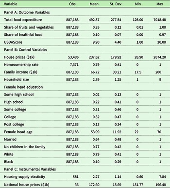
Table 1 lists the 23 food groups used in constructing our household-level diet variables. In this table, we show the expenditure share of average households in our sample and the recommended share for a representative household.Footnote 5 As is shown, the expenditure shares in the healthful food groups – dark vegetables, fruits, canned and dry beans, lentils, peas, and white meat – are consistently below the amounts recommended by USDA, while households consume significantly more than is recommended from the unhealthful categories – soft drinks, sodas, fruit drinks, sugars, sweets, candies, and frozen or refrigerated dinners. Overall, the total expenditure on healthful food is 35%, while the recommended share is 82%.
Table 2 presents summary statistics for the variables used in our econometric analysis. The sample we use in this study comprises 887,183 household-quarter observations. Panel A shows the descriptive statistics for our outcome variables; Panel B provides summary statistics for our control variables; and Panel C provides summary information for our instrumental variables.
Table 2. Summary Statistics

Note: The above summary is based on the quarterly data we organized from Nielsen HomeScan household panel for the years 2005–2013. The Nielsen HomeSacn data are not representative for the US population. Comparing to US population, our data include more households with higher age and living in metropolitan areas.
Econometric model
Baseline model
To identify the impact of house price shocks on food expenditure and dietary outcomes, we begin with the following baseline linear specification:
 $${Y_{hzq}} = {\beta _0} + {\beta _1}lnH{P_{zq}} + {X_{hq}}\delta + {\lambda _h} + {\mu _q} + {\varepsilon _{hzq}},$$
where ${Y_{hzq}}$
represents our outcome variab le of interest for household
${Y_{hzq}}$
represents our outcome variab le of interest for household $h$
, in zip code
$h$
, in zip code $z$
, in quarter
$z$
, in quarter $q$
;
$q$
; $lnH{P_{zq}}$
is the natural log of house prices at the zip code level in quarter
$lnH{P_{zq}}$
is the natural log of house prices at the zip code level in quarter $q$
;
$q$
; ${X_{hq}}$
is a vector of control variables;
${X_{hq}}$
is a vector of control variables; ${\lambda _h}$
is a household fixed effect;
${\lambda _h}$
is a household fixed effect; ${\mu _q}$
is quarterly fixed effect; and
${\mu _q}$
is quarterly fixed effect; and ${\varepsilon _{hzq}}$
is an error term. The control variable
${\varepsilon _{hzq}}$
is an error term. The control variable $Xhq$
includes family income, household size, dummies indicating a household head’s education level, household head’s age, a dummy indicating the household head’s marital status, a dummy indicating the presence of children, and dummies for race. To ensure that our results are not driven by households migrating between zip codes, we consider the same household living in different zip codes in different periods as separate observations. Therefore, we track diet changes for the same household in the same zip code using household fixed effects
$Xhq$
includes family income, household size, dummies indicating a household head’s education level, household head’s age, a dummy indicating the household head’s marital status, a dummy indicating the presence of children, and dummies for race. To ensure that our results are not driven by households migrating between zip codes, we consider the same household living in different zip codes in different periods as separate observations. Therefore, we track diet changes for the same household in the same zip code using household fixed effects ${\lambda _q}$
. In this way, we are able to avoid selection bias as households who value health may move to more expensive communities with a better food environment. Finally, we control for quarter fixed effects
${\lambda _q}$
. In this way, we are able to avoid selection bias as households who value health may move to more expensive communities with a better food environment. Finally, we control for quarter fixed effects ${\mu _q}$
to capture time-varying macro shocks.
${\mu _q}$
to capture time-varying macro shocks. ${\beta _1}$
, which is our coefficient of interest, represents the elasticity of dietary outcomes with respect to house prices.
${\beta _1}$
, which is our coefficient of interest, represents the elasticity of dietary outcomes with respect to house prices.
Owners vs. renters model
Theory suggests that changes in house prices may impact expenditure on other goods and services through wealth or collateral channels – changes in asset prices (housing) relax borrowing and budget constraints and change expenditure on other goods as a result of increased income. This result, however, should only hold for asset owners, or homeowners in our case. Thus, we do not expect a positive relationship to exist between house prices and food expenditure for renters. To exploit these differential responses, we estimate the following model:
 $${Y_{hzq}} = {\beta _0} + {\beta _1}lnH{P_{zq}}*ow{n_{hz}} + {\beta _2}lnH{P_{zq}} + {X_{hq}}\delta + {\lambda _h} + {\mu _q} + {\varepsilon _{hzq}},$$
where $ow{n_{hz}}$
represents the homeownership status for household
$ow{n_{hz}}$
represents the homeownership status for household $h$
in zip code
$h$
in zip code $z$
,
$z$
, ${\beta _2}$
shows how changes in house prices affect the dietary outcomes of renters, and
${\beta _2}$
shows how changes in house prices affect the dietary outcomes of renters, and ${\beta _1}$
captures the differential effect of house prices on homeowners. We expect
${\beta _1}$
captures the differential effect of house prices on homeowners. We expect ${\beta _1}$
to be positive based on the theory discussed above. As our data do not provide direct information on the homeownership status of each household, we use two distinct strategies to identify homeowners. First, we use homeownership rates at the zip-code level as a proxy for homeownership. In this setting, we exploit variation in homeownership rates across zip codes – i.e., we expect house price changes to have a differential effect for households living in areas with different rates of homeownership. Second, we use the house-type variable (defined as single-family or multi-family residences) in the Nielsen data and follow Stroebel and Vavra (Reference Stroebel and Vavra2019) to determine whether a household is a renter or owner. Specifically, we identify households living in one-family and non-condo residences as homeowners and families living in 3+ family residences as renters.
${\beta _1}$
to be positive based on the theory discussed above. As our data do not provide direct information on the homeownership status of each household, we use two distinct strategies to identify homeowners. First, we use homeownership rates at the zip-code level as a proxy for homeownership. In this setting, we exploit variation in homeownership rates across zip codes – i.e., we expect house price changes to have a differential effect for households living in areas with different rates of homeownership. Second, we use the house-type variable (defined as single-family or multi-family residences) in the Nielsen data and follow Stroebel and Vavra (Reference Stroebel and Vavra2019) to determine whether a household is a renter or owner. Specifically, we identify households living in one-family and non-condo residences as homeowners and families living in 3+ family residences as renters.
Instrumental variable model
The estimates from Equations (1) and (2) are unbiased if house prices are exogenous. Here, endogeneity may arise for several reasons. First, common factors such as financial liberalization and expectation over future income are likely to drive up house prices and food consumption simultaneously (Campbell and Cocco Reference Campbell and Cocco2007). Conversely, omitted variables on time allocated to shopping are likely to be negatively correlated with house prices but have a positive effect on food spending. To address these issues, we extend our baseline and homeowner-renter specifications and estimate an instrumental variable (IV) model.
Following Mian et al. (Reference Mian, Rao and Sufi2013), Dettling and Kearney (Reference Dettling and Kearney2014), Chetty et al. (Reference Chetty, Sándor and Szeidl2017), Aladangady (Reference Aladangady2017), and Guren et al. (Reference Guren, McKay, Nakamura and Steinsson2021), we use the interaction of MSA-level housing supply elasticities and national house price trends as an instrument for house prices in Equations (1) and (2). The housing supply elasticity is from Saiz (Reference Saiz2010), and the variance of the housing supply elasticity contains two parts. The first part comes from exogenous geographic features, such as water, oceans, mountains, and wetlands, which are used to measure unavailability of the land. The second part is take from the Wharton Residential Urban Land Regulation Index created by Gyourko et al. (Reference Gyourko, Saiz and Summers2008). The index is used to capture the stringency of residential growth controls. As we use fixed-effect panel data, we build a shift-share instrumental variable by interacting the housing supply elasticities with national house prices. The intuition is that when there are macro-level positive demand shocks to housing, high housing supply elasticity areas, such as Texas, Arizona, and Georgia, experience less of a house-price shock compared to low housing supply elasticity areas, such as California and Massachusetts.
This instrumental variable is not without its limitations. Davidoff (Reference Davidoff2015) points out that housing supply elasticities can be related to other city characteristics and therefore are correlated with long-run growth in demand. Thus, it will pose a problem for cross-sectional analysis. However, our study employs the fixed-effect model using panel data and can overcome this issue. In addtion, Guren et al. (Reference Guren, McKay, Nakamura and Steinsson2021) show that the housing supply elasticity from Saiz (Reference Saiz2010) may lose power for the data before 2000. Our study avoids this time period.
We estimate our IV model using two-stage least squares (2SLS). The first stage of our IV model is specified as follows:
 $$lnH{P_{zq}} = {\alpha _0} + {\alpha _1}Elasticit{y_{MSA}}*lnH{P_q} + {X_{hq}}{\delta _1} + {\lambda _h} + {\mu _q} + {e_{hzq}},$$
where $Elasticit{y_{MSA}}$
represents the housing supply elasticity at the MSA level and
$Elasticit{y_{MSA}}$
represents the housing supply elasticity at the MSA level and $lnH{P_q}$
is our national house price index in quarter
$lnH{P_q}$
is our national house price index in quarter $q$
. After estimating equation (3), we obtain predicted values of our endogenous house-price variable and estimate the following second-stage model:
$q$
. After estimating equation (3), we obtain predicted values of our endogenous house-price variable and estimate the following second-stage model:
 $${Y_{hzq}} = {\beta _0} + {\beta _1} {lnH{P_{zq}}} + {X_{hq}}\delta + {\lambda _h} + {\mu _q} + {\varepsilon _{hzq}},$$
where ${lnH{P_{zq}}}$
is the predicted value for
${lnH{P_{zq}}}$
is the predicted value for $lnH{P_{zq}}$
from the first stage.
$lnH{P_{zq}}$
from the first stage.
To handle price endogeneity in Equation (2), we need two instruments – one for house prices and the other one for the interaction between house prices and homeownership. We follow Dettling and Kearney (Reference Dettling and Kearney2014) and add a second IV to our model by using the interaction of housing supply elasticity, national house prices, and our indicator for homeownership. The first stage of our homeowner–renter IV model consists of two linear regressions given by:
 $$\matrix{
{lnH{P_{zq}} = {\alpha _0} + {\alpha _1}Elasticit{y_{MSA}}*lnH{P_q} + {\alpha _2}Elasticit{y_{MSA}}*lnH{P_q}*ow{n_{hz}}} \hfill \cr
{\quad \quad \quad \quad + {X_{hq}}{\delta _1} + {\lambda _h} + {\mu _q} + {e_{hzq}}} \hfill \cr
} $$
$$\matrix{
{lnH{P_{zq}} = {\alpha _0} + {\alpha _1}Elasticit{y_{MSA}}*lnH{P_q} + {\alpha _2}Elasticit{y_{MSA}}*lnH{P_q}*ow{n_{hz}}} \hfill \cr
{\quad \quad \quad \quad + {X_{hq}}{\delta _1} + {\lambda _h} + {\mu _q} + {e_{hzq}}} \hfill \cr
} $$
and
 $$\matrix{
{lnH{P_{zq}}*ow{n_{hz}} = {\gamma _0} + {\gamma _1}Elasticit{y_{MSA}}*lnH{P_q} + {\gamma _2}Elasticit{y_{MSA}}*lnH{P_q}*ow{n_{hz}}} \hfill \cr
{\quad \quad \quad \quad \quad \quad \quad + {X_{hq}}{\delta _2} + {\lambda _h} + {\mu _q} + {\upsilon _{hzq}},} \hfill \cr
} $$
$$\matrix{
{lnH{P_{zq}}*ow{n_{hz}} = {\gamma _0} + {\gamma _1}Elasticit{y_{MSA}}*lnH{P_q} + {\gamma _2}Elasticit{y_{MSA}}*lnH{P_q}*ow{n_{hz}}} \hfill \cr
{\quad \quad \quad \quad \quad \quad \quad + {X_{hq}}{\delta _2} + {\lambda _h} + {\mu _q} + {\upsilon _{hzq}},} \hfill \cr
} $$
where $lnH{P_{zq}}$
and
$lnH{P_{zq}}$
and $lnH{P_{zq}}*ow{n_{hz}}$
are both endogenous variables with instruments given by
$lnH{P_{zq}}*ow{n_{hz}}$
are both endogenous variables with instruments given by $Elasticit{y_{MSA}}*lnH{P_q}$
and
$Elasticit{y_{MSA}}*lnH{P_q}$
and $Elasticit{y_{MSA}}*lnH{P_q}*ow{n_{hz}}$
.
$Elasticit{y_{MSA}}*lnH{P_q}*ow{n_{hz}}$
.
The second stage of our homeowner–renter IV model is given by
 $$\matrix{
{{Y_{hzq}} = {\beta _0} + {\beta _1}lnH{P_{zq}}*ow{n_{hz}} + {\beta _2}lnH{P_{zq}}} \hfill \cr
{\quad \;\; + {X_{hq}}\delta + {\lambda _h} + {\mu _q} + {\varepsilon _{hzq}},} \hfill \cr
} $$
$$\matrix{
{{Y_{hzq}} = {\beta _0} + {\beta _1}lnH{P_{zq}}*ow{n_{hz}} + {\beta _2}lnH{P_{zq}}} \hfill \cr
{\quad \;\; + {X_{hq}}\delta + {\lambda _h} + {\mu _q} + {\varepsilon _{hzq}},} \hfill \cr
} $$
where $ {lnH{P_{zq}}*ow{n_{hz}}}$
and
$ {lnH{P_{zq}}*ow{n_{hz}}}$
and $ {lnH{P_{zq}}}$
are predicted values for
$ {lnH{P_{zq}}}$
are predicted values for $lnH{P_{zq}}*ow{n_{hz}}$
and
$lnH{P_{zq}}*ow{n_{hz}}$
and $lnH{P_{zq}}$
from equations (5) and (6).
$lnH{P_{zq}}$
from equations (5) and (6).
Results
The results from our baseline model (Equation 1) are shown in Table 3. Column 1 shows results for total expenditure (column 1) and columns (2)–(4) show results for dietary outcomes. All models are estimated in log–log form, so the coefficients represent elasticities. We find that a 1% increase in house prices leads to 0.018% increase in total quarterly food expenditure. We do not find any statistically significant effect on diet quality measures.
Table 3. Results for Baseline Model

Note: This table presents results for our baseline specification (Equation 1). Outcome variables are shown across the top. Household controls include family income, household size, a dummy for the education level of the household head, household head’s age, a indicator for marital status, a indicator for the presence of children, and race dummies. Robust standard errors are shown in parentheses and clustered at the zip-code level. *Significant at 10% level. **Significant at 5% level. ***Significant at 1% level.
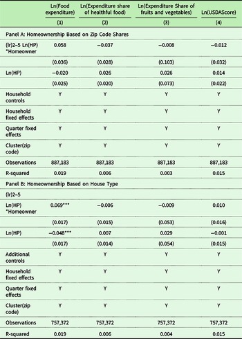
Table 4 shows results for our homeowner–renter specification (Equation 2). Panel A shows results with homeownership based on zip-code-level homeownership rates, and Panel B reports results where we define homeownership based on home types. As stated above, we define homeowners as households living in one-family, non-condo residences, and renters as households living in 3+ family residences. From column (1) of Panel A and Panel B, we observe, consistent with theory, that the effect of house prices on food expenditure for homeowners is positive, while the effect for renters is negative. However, this effect is only significant for Panel B, where we use house type to define ownership. From Panel B, we find that a 1% increase in house value leads to a 0.048% reduction in expenditure for renters and a 0.021% increase in expenditure for homeowners. Once again, across all models we do not find any significant impact of house price shocks on diet quality.
Table 4. Results for Homeowners vs. Renters Model

Note: This table presents results for our homeowner-renter specification (Equation 2). Panel A presents results for a model with ownership defined based on zip-code-level homeownership rates and Panel B presents results for a model where we define homeowners based on their type of residence. Household controls are the same as in Table 3. Robust standard errors are in parentheses and they are clustered at zip-code level. *Significant at 10% level. **Significant at 5% level. ***Significant at 1% level.
As noted previously, it is likely that our house price estimates are biased. To address this, we estimate a series of IV models for our baseline and homeowner-renter models using an interaction between MSA-level housing supply elasticities and national house prices as an instrument (Dettling and Kearney Reference Dettling and Kearney2014; Chetty et al. Reference Chetty, Sándor and Szeidl2017; Stroebel and Vavra Reference Stroebel and Vavra2019). The first-stage results for all of our IV models are shown in Table 5. Column (1) presents results for our baseline model, and columns (2)–(5) provide results for our homeowner–renter specifications. From these results, we can see that our instrumental variable has a significant and negative effect on house prices. This result suggests that house prices in areas with higher housing supply elasticities increase less than in areas with lower supply elasticities following a national housing demand shock. This is consistent with urban spatial theory. We also find that our weak instrument tests – F-tests – are at or above the results specified in Stock and Yogo (Reference Stock and Yogo2002). Using these results, we proceed with the estimation of our IV models.
Table 5. First-Stage Results - IV

Note: This table presents results from our first-stage IV model. Column (1) reports the results from equation (3) and column (2)–(5) show the estimates from equation (5) and (6). In columns (2) and (3) the ,homeownership is the homeownership rate at the zip code level and in columns (4) and (5) the homeownership is the household-level homeownership based on the house type. Robust standard errors are in parentheses. *Significant at 10% level. **Significant at 5% level. ***Significant at 1% level.
Table 6 presents results for our baseline model estimated in IV form. Here, we find a positive and significant impact of house price shocks on total food expenditure, but the impacts remain statistically insignificant for diet quality. Further, we find that after instrumenting for house prices food expenditure elasticity increases over three times in comparison to the non-IV model in Table 3. Specifically, we find that for 1% increase in house price food expenditure increases by 0.057% in the IV model, compared to only 0.018% in the non-IV baseline model. Converting the elasticity value in Table 6 into an actual expenditure amount suggests that households will increase their total yearly expenditures on food by $0.00047 and increase overall household expenditure by $0.014 for every $1 increase in housing value. Footnote 6
Table 6. Results for Baseline IV Model

Note: This table presents the estimates from the second-stage regression based on the effect of equation (4). Robust standard errors are in parentheses and they are clustered at zip-code level. *Significant at 10% level. **Significant at 5% level. ***Significant at 1% level.
Table 7 presents second-stage results for our homeowner–renter IV model. Panel A is for a model where homeownership is based on zip-code shares, and Panel B is for homeownership based on house type. The results for total expenditure are similar to those in Table 4, but now we find a positive and statistically significant result for homeowners across both home ownership designations. Specifically, we find that the food expenditure elasticity for house prices for homeowners is 0.204 in Panel A and 0.125 in Panel B. For total expenditure, an elasticity value of 0.125–0.204 translates into a $0.0009–$0.0012 increase in food expenditure and a $0.025–$0.03 increase in total expenditure for a $1 increase in house value. We find no statistically significant results for renters. From Columns (2)–(4), the estimated impact of house prices on diet quality are not significant for owners or renters once again suggesting that higher house prices, which shock household budgets, do not translate into improvements in diet quality.
Table 7. Results for IV Homeowners vs. Renters Model

Note: This table presents the estimates from the second-stage regression based on the equation (7). Panel A shows the results when we use zip-code-level homeownership rate and Panel B reports the results when we use the homeowner based on the house type. Robust standard errors are in parentheses and they are clustered at zip-code level. *Significant at 10% level. **Significant at 5% level. ***Significant at 1% level.
To summarize the results presented in Tables 3–7, we find that house price shocks have a positive impact on overall food expenditure. These results hold across all of our non-IV and IV models. Conversely, in none of our models did we find that house price shocks change the quality of the food households purchase. The sign and magnitude of our results related to total expenditure are consistent with previous research (Mian et al. Reference Mian, Rao and Sufi2013; Aladangady Reference Aladangady2017). Specifically, recent empirical studies have shown that consumption elasticities with respect to changes in house prices range from 0.03 to 0.26 (Case et al. Reference Case, Quigley and Shiller2011; Carroll et al. Reference Carroll, Otsuka and Slacalek2011; Mian et al. Reference Mian, Rao and Sufi2013); we find that elasticities in our model range from 0.125 to 0.204. Thus, overall our estimates of the impact of changes in house prices on total and food expenditure are similar to previous studies, which lends further credibility to our results related to diet quality. Our diet quality results are also consistent with several recent studies showing that household diet quality is stable and is not affected by the factors such as improved access, increased budgets, serious disease diagnosis, or changes in government diet recommendations (Kozlova Reference Kozlova2016; Atkin Reference Atkin2016; Allcott et al. Reference Allcott, Diamond, Dubé, Handbury, Rahkovsky and Schnell2019; Hastings et al. Reference Hastings, Kessler and Shapiro2021; Hut and Oster Reference Hut and Oster2022).
Robustness checks
While the results in the previous section appear consistent across models, we conduct additional robustness checks by utilizing a series of alternative models and variable specifications
One possible explanation for our results, that house prices only affect food spending rather than diet quality, is that the spending increase is mainly driven by food price changes. Therefore, the real budget for food may not change. If this is the case, households should consume the same amount of the food as before. In order to deal with this concern, we directly check the effects of house prices on the total quantity of the food. In our household consumption data, over 90% of food purchases have weight values. Using these data, we examine the effect of house price shocks on the weight of food purchased. The results from this model are shown in Table 8. Column (1) presents the results for our baseline IV model where the total food expenditure is replaced by total food quantity; columns (2) and (3) present the results from our homeowner–renter IV model. The food weight elasticity for homeowners is in the range of 0.066–0.095 and the food expenditure elasticity is 0.096–0.124. Therefore, we conclude that the food expenditure changes found in the previous section are mainly driven by changes in total food quantity and not by changes in food prices; households simply buy more food as budget constraints are relaxed.
Table 8. Robustness Check: Expenditure vs. Quantity

Note: This table presents results for our food quantity IV model, where we examine the impact of house price shocks on the total quantity of food consumed and not on expenditure. Robust standard errors are in parentheses and they are clustered at the zip code level. *Significant at 10% level. **Significant at 5% level. ***Significant at 1% level.
The remainder of our robustness check models are shown in Table 9. First, we replace quarterly household food expenditures with yearly expenditures. The purpose is to avoid seasonality effects. Panel A shows the results for our IV homeowner-renter model using yearly data. Footnote 7 The results are similar to the model estimated using quarterly data – the coefficient on house prices for owners is 0.127, the impact on renters is insignificant, and there is no effect of house prices on diet quality.
Table 9. Other Robustness Checks

Note: This table presents the results for a series of robustness checks. We use the IV homeowner–renter model and separate homeowners and renters based on the house type. Panel A reports the estimates when we use yearly rather than quarterly data; Panel B reports estimates for a model after excluding observations from California, Florida, and Arizona, which experience largest house price boom and bust. Robust standard errors are in parentheses and they are clustered at the zip code level. *Significant at 10% level. **Significant at 5% level. ***Significant at 1% level.
Second, we test whether our results are mainly driven by some cities with extreme boom-bust housing cycles. In Panel B of Table 9, we drop observations from California, Arizona and Florida and re-estimate our IV homeowner–renter model. The results from this model are consistent with the model using the full sample.
Last, we investigate the effect of house prices on the expenditure shares of each food category separately. Table 10 shows results for healthful categories and Table 11 shows results for unhealthful categories. As we can see, the expenditure shares of almost every food category is unaffected by house prices, which supports our main results that house prices have no impact on diet structure and quality.
Table 10. Results for Model with All Healthful Food Categories

Note: This table presents the effects of house prices on the expenditure share of healthful food. We use the IV homeowner–renter model and separate homeowners and renters based on the house type. Robust standard errors are in parentheses and they are clustered at the zip code level. *Significant at 10% level. **Significant at 5% level. ***Significant at 1% level.
Table 11. Results for Model with All Unhealthful Food Categories

Note: This table presents the effects of house prices on the expenditure share of unhealthful food. We use the IV homeowner–renter model and separate homeowners and renters based on the house type. Robust standard errors are in parentheses and they are clustered at the zip code level. *Significant at 10% level. **Significant at 5% level. ***Significant at 1% level.
Results heterogeneity
One main advantage of using microdata is that we can investigate the effects for subgroups of the population. Although our results show that house prices have a positive effect on food expenditure and do not have a significant effect on diet quality, households in different demographic groups may respond differently to house price fluctuations. In this section, we explore the heterogeneity effects across income and age groups. To provide a comparison with previous results, we estimate equations (5), (6), and (7) and separate homeowners and renters based on the house type.
Income
In this part, we examine the effect of house prices on dietary outcomes for different income groups. Kozlova (Reference Kozlova2016) splits the sample into three different income groups: below 130%, above 130% and below 200%, and above 200% of the poverty threshold. These cutoffs have important policy implications. For example, households qualify for the Supplemental Nutrition Assistance Program (SNAP) if their income is below 130% of poverty threshold. Households economically struggle once their income lies below 200% of the poverty threshold. In this study, we divide the sample into income groups below and above 200% of the poverty threshold as we have excluded the observations with income below 130%. As lower income households are more likely to be budget constrained, we expect that house prices will have a larger impact on them compared to households with higher incomes.
Panels A and B of Table 12 present estimates for households below and above 200% of the poverty threshold, respectively. Column (1) reports the effects of house prices on food expenditure. From Panel A, we find that house prices have a significant effect on food expenditure for homeowners and insignificant effect on renters. The food expenditure elasticity is around 0.135 for lower income homeowners. The estimates from Panel B suggest that the food expenditure elasticity of house prices is around 0.126 for homeowners whose incomes lies above 200% of the poverty line. The effects for renters are insignificant for both income groups, which is consistent with previous results. Column (2)–(4) of the table show the effects of house price shocks on diet quality. The effects are not significant in most regressions, although we do find a positive effect for lower income households for the expenditures on of fruits and vegetables.
Table 12. Results for Income Heterogeneity Model

Note: This table presents results for our IV homeowner–renter model for different income groups. We identify homeowners based on the house type. Panel A shows estimates for the sample under the 200% poverty threshold and panel B shows results for households greater than 200% of the poverty line. We identify homeowners based on the house type. Robust standard errors are in parentheses. *Significant at 10% level. **Significant at 5% level. ***Significant at 1% level.
Age
In this part, we divide the sample into two groups according to the age of household heads: above and below 50. Footnote 8 Differential consumption reactions to house-price shocks between younger and older households would suggest the major mechanism by which house prices affect consumption. For example, if the effect is larger for older homeowners, it would suggest that the wealth effect may play a larger role than the collateral effect. This is because older homeowners have strong incentives to sell their large houses and move to small ones with the family size decreasing (Campbell and Cocco Reference Campbell and Cocco2007). If younger homeowners are more affected by house price changes, then the collateral effect is probably the main driver since younger households are more likely to face borrowing constraints. Thus, relaxed borrowing constraints, driven by increasing house prices, would stimulate more spending for younger homeowners as compared to older homeowners.
Table 13 reports our results for different age groups. Column (1) shows that house prices have a positive and significant effect for both younger and older homeowners, while the effects for renters are not significant. The food expenditure elasticity of house prices is 0.135 for homeowners with the household head under 50, and the elasticity is 0.097 for homeowners with the household head over 50. Again, we do not find any evidence that house prices have a significant impact on diet quality in any age group.
Table 13. Results for Age Heterogeneity Model

Note: This table presents results for our IV homeowner-renter model for different age groups based on the household head. We identify homeowners based on the house type. Panel A is for the younger households defined as a household head with age below 50 and Panel B is for the older households with household head age above 50. We identify homeowners based on the house type. Robust standard errors are in parentheses and they are clustered at the zip code level. *Significant at 10% level. **Significant at 5% level. ***Significant at 1% level.
Taken together, we find that the effect of house prices on food expenditure is larger in lower income and younger groups. This suggests that house prices affect food expenditure mainly through the collateral effect rather than the wealth effect as lower income and younger households are more likely to be in borrowing constraints. Aladangady (Reference Aladangady2017) and Berger et al. (Reference Berger, Guerrieri, Lorenzoni and Vavra2018) also find similar results. In addition, we show that house prices do not affect diet quality even in those groups whose food expenditures experience the largest change. This further confirms our conclusion that relaxing budget constraints is not effective in improving diet quality.
Conclusions
In this paper, we examine how wealth shocks driven by house price movements impact household food consumption. We are specifically interested in how these shocks impact both overall food expenditure and diet quality. To answer these questions, we use a nationally representative consumer expenditure panel data set from Nielsen (HomeScan) matched with zip-code-level house prices. To deal with endogeneity issues associated with our house-price variable, we use MSA-level housing supply elasticities interacted with national time-series of house prices as an instrumental variable. We also exploit differences between homeowners and renters.
The results from our model show that the house price elasticities with respect to food expenditure are 0.057 for the average household and 0.125–0.204 for homeowners. The quality of the food, however, is not affected by changes in house prices. We also look at how house prices impact the quantity of food consumed and the expenditure share of each food category. The results show that house prices have positive effects on food weight, but do not change the food structure. Finally, we conduct the heterogeneity analysis to look at how house prices affect food consumption differently within several subgroups in the population. We find that the effect of house prices on food expenditure is larger for lower income and younger household groups, but, once again, we find no impact on diet quality within these groups.
Our results, showing a positive and significant effect of house prices on food spending, is in line with the findings from previous studies. The results on budget constraints and diet quality, however, are different from previous literature. The negligible relationship between house prices and diet quality can be attributed to several causes. First, eating habits may be difficult to alter. Recent studies have shown that households’ diets are not malleable (Kozlova Reference Kozlova2016; Atkin Reference Atkin2016; Allcott et al. Reference Allcott, Diamond, Dubé, Handbury, Rahkovsky and Schnell2019; Hut and Oster Reference Hut and Oster2022). Hut and Oster (Reference Hut and Oster2022) show that only 5% of households have significantly changed their diets in the Nielsen HomeScan panel. Second, diet may not be impacted by short-run income or wealth shocks and be more dependent on permanent or long-run changes to income. Allcott et al. (Reference Allcott, Diamond, Dubé, Handbury, Rahkovsky and Schnell2019) suggest that the positive nutrition-income relationship found in the public health literature is likely explained by the long-term effects of income and not by short-term effects. Controlling for household fixed effects, we mostly estimate a short-term relationship between housing wealth and consumption and thus our results support this conclusion.
While our study provides important insights, it has some limitations. First, the Nielsen HomeScan panel data do not include food away from home. Although Allcott et al. (Reference Allcott, Diamond, Dubé, Handbury, Rahkovsky and Schnell2019) find that grocery purchases are not a systematically biased measure of overall diet healthfulness, it is still necessary to reexamine the effects using data including both food at home and away from home. And second, our measure of diet quality may be measured with error. All three of our diet quality measures are based on expenditure shares. While expenditure-based measures have their advantages, they have the tendency to be impacted by price changes. Thus, it will be important to include other measures, such as nutrition, in future work.
Data
Researcher(s) own analyses calculated (or derived) based in part on data from The Nielsen Company (US), LLC and marketing databases provided through the Nielsen Datasets at the Kilts Center for Marketing Data Center at The University of Chicago Booth School of Business. The conclusions drawn from the Nielsen data are those of the researcher(s) and do not reflect the views of Nielsen. Nielsen is not responsible for, had no role in, and was not involved in analyzing and preparing the results reported herein.
Funding statement
This material is based on work that is supported by the Multistate Project (W4133) from the U.S. Department of Agriculture National Institute of Food and Agriculture through the project “Costs and Benefits of Natural Resources on Public and Private Lands: Management, Economic Valuation, and Integrated Decision Making.”
Competing interests
None.


 Open access