


Introduction
The scanning electron microscope (SEM) is widely used in various fields of industry and science because it is one of the most versatile imaging and measurement tools. Images produced are particularly appreciated for their high depth of field and excellent image resolution, both orders of magnitude better than light microscopy. However, images provided by the SEM are black and white, and single images contain information in only two dimensions. Of course grayscale images from an SEM are normal since this technology forms images with electrons instead of photons of visible light. Yet color is something important to us humans, and not just from an aesthetic point of view. For millions of years perception of color helped our ancestors to survive, for example by allowing them to distinguish a ripe fruit hidden amongst the green leaves of a tree. Color helps our brain to differentiate and identify objects. Thus our brains rely on color (and stereoscopic vision) to correctly perceive objects.
When it comes to viewing the nanoscopic world, researchers spend hours of their precious time manually “colorizing” SEM images in order to more clearly communicate their findings to other humans.
But that could soon change. Thanks to the increasing power of computer software and computer graphics, the technology surrounding electron microscopes is gradually moving toward both color and 3D. Of course, whether color is applied manually or semi-automatically, the researcher has a responsibility not to cause misinterpretation of the data. Applying colors that were not present in the original image can change the viewer’s impression of the data, so the original image always should remain available to the viewer.This article describes how color (and 3D) can be added to SEM images using both traditional techniques and modern computer methods. Note: scale bars have been eliminated from some images in this article in order to concentrate on the image processing.
Colorization Methods
In an SEM image, the signal intensity at each pixel corresponds to a single number that represents the proportional number of electrons emitted from the surface at that pixel location. This number is usually represented as a grayscale value, and the overall result is a black-and-white image. Of course, color can be used to encode existing SEM images with extra information coming from other physical data, such as characteristic X-ray emission or cathodoluminescence spectrometry. Color has also been added by mixing the signals from multiple electron detectors, each detector coded for a different color [Reference Scharf1]. But the question is: how does one go about colorizing SEM images with only the information contained within the SEM images themselves?
Pseudocolor
The numbers representing each pixel intensity can be arbitrarily matched to a color via a lookup table. This is known as pseudocolor or “false color.” Lookup tables may be based on the colors of the rainbow (blue-green-yellow-orange-red-white), the colors of the thermal scale (black, red, orange, white), or some arbitrary color scale [Reference Goldstein2]. Using this approach obviously doesn’t add any additional information to the image, but it can allow better visualization of image detail (or material phases) in a sample. This is the case when color is applied to SEM backscattered electron (BSE) images in which image brightness increases with increasing atom number in the specimen. Figure 1a shows a raw BSE image displayed in grayscale. This image exhibits non-uniform brightness, the right side being visibly darker than the left. In Figure 1b, false color has been added by arbitrarily matching a color to each gray level; however, because the gray levels were not uniform across the field, it is not possible to distinguish the phases confidently at this stage. Figure 1c shows the result of applying mathematical correction of the gray levels. This type of image processing consists of subtracting the 2nd degree polynomial that best fits (least square method) the homogeneous (low variance) areas of the gray-level image. In the corrected image, each color represents a different mineral phase that can yield a quantitative volume fraction.
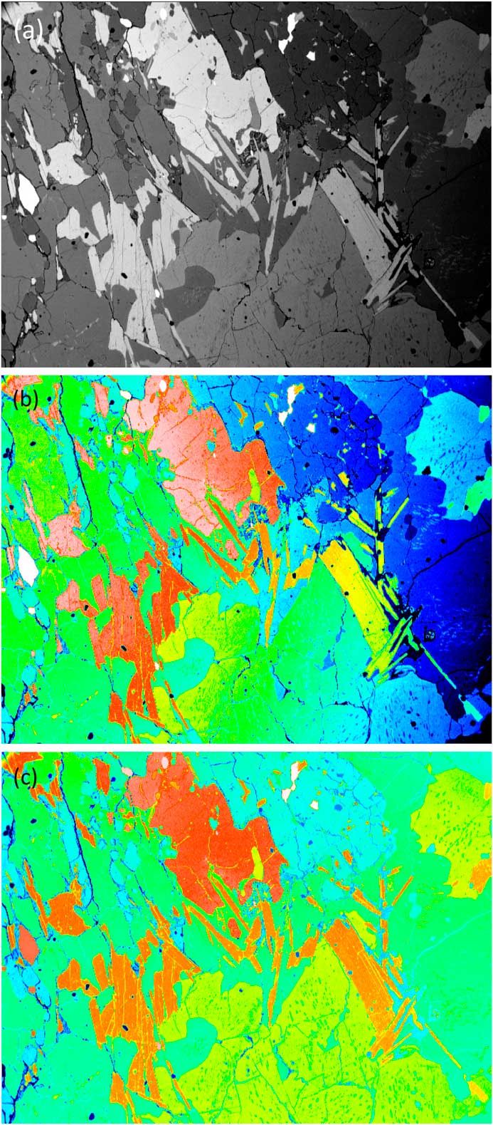
Figure 1 SEM images using the BSE signal from a flat-polished specimen containing several mineral phases. (a) Raw image in grayscale. (b) False color image where a color was arbitrarily assigned to each gray level. (c) Mathematically corrected image where each color represents a different mineral phase. Original image courtesy of the School of Geosciences, University of Edinburgh.
Image superposition
A BSE image with strong compositional contrast also can be superimposed onto a secondary electron (SE) image. The result is a composite or mixed image in which the texture and composition of a sample are both visible: composition being represented by false color differences, while topographical differences show up in the details of the shadowing (Figure 2). This is known as a density-dependent color scanning electron micrograph (DDC-SEM) [Reference Bertazzo3].
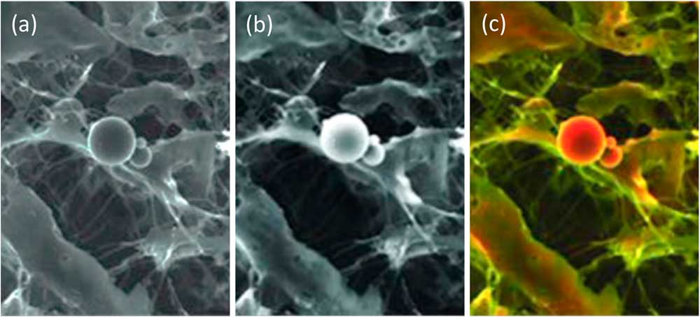
Figure 2 Image of calcified particles in cardiac tissue. (a) Secondary electron (SE) SEM image, (b) BSE image, (c) DDC-SEM image obtained by superimposing the two previous images and adding color to the BSE image via a lookup table. This colorization technique helps to reveal both the composition and texture of the sample. Original images courtesy of Sergio Bertazzo.
Manual colorization
Another approach for SE images is to manually colorize objects. Once an SEM image is obtained, researchers may spend considerable time identifying, isolating, and colorizing each type of object so that readers of their publications are able to instinctively comprehend and interpret them. The problem, of course, is that this is usually a tedious and time-consuming operation. Each object has to be manually separated from the others, for example using image-editing software.
Semi-automated colorization
One recent technique allows users to colorize images quickly and easily. MountainsMap SEM allows automatic or semi-automatic object identification and segmentation. Selecting an object can often be achieved with just one click of the mouse. The technology behind this step involves over 30 successive mathematical operations to distinguish the various objects in the image (Figure 3).
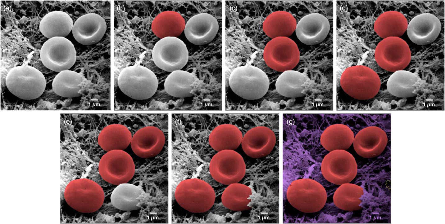
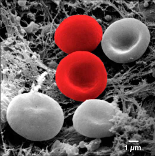
Figure 3 Image of erythrocytes (red blood cells). Images from left to right show a sequence of stages in the colorization process using MountainsMap® SEM software. From one step to the next required only a single mouse click. Original image courtesy of Thierry Thomasset, Université Technologique de Compiègne.
The final image in Figure 3 could potentially take hours to produce using photo-editing software. Of course, whether or not two adjacent objects should be separated can be open to interpretation. For instance, should a blackberry be considered one fruit or many fruits? (Not sure our ancestors asked themselves this before eating them . . .). Thankfully, the software allows users to define and modify boundaries around objects. This is accomplished by varying the settings on object size filters, by using free border editing (mouse drawing and cutting), or by picking from among secondary boundaries (as one would differentiate state borders from county boundaries within the state). Of course, the example presented here (Figure 3) is a relatively easy one. Not all objects can be picked up in a single mouse click. But even if three or four clicks are necessary to indicate to the software that certain parts go together, it is still much quicker than having to draw around objects manually.
Furthermore, in the case of multiple similar objects, the software can find them automatically and allocate a color to each depending upon its size or shape. For example, on a black and white photograph, it would color all the rice white and the peas green automatically based on their shape. In another image, it would color all the grapefruits in yellow and all the tangerines in orange based on their size, once an example of each has been shown as a model.
Leaving the Flat World
From 2D to 3D
There are several methods for converting standard two-dimensional (SE) images into 3D-like images (that is, those representing X, Y, and Z (height) coordinates). Color can be closely linked to this process.
Stereophotogrammetry
The most metrologically accurate approach to 3D reconstruction of surface features is stereophotogrammetry. This technique consists of acquiring two SEM images of the same object from different angles. Height information can then be calculated trigonometrically. The only drawbacks of this method are that it requires having an SEM that allows specimen tilt and calls for two successive images of the sample to be taken (Figure 4a). A number of commercial and non-commercial software solutions are available to interpret the 3D information in the stereo pair. Figure 4b shows a perspective reconstruction produced by MountainsMap SEM. The topography obtained allows the quantification of surface features (step height, volume, angles, flatness). This 3D representation was obtained by (1) calculating a topography map from the stereo reconstruction, (2) creating a distorted 3D mesh out of this topography model, (3) pasting the original left SEM image onto it, and (4) colorizing it with a brown false color from the map height and shading. Figure 4c shows a profile through the 3D representation corresponding to a cross section of the 3D reconstruction. This example demonstrates the ability of the method to accurately add a third dimension to a pair SEM stereo images, provided there is enough local texture [Reference Vipin4]. The Ra value determined by software here matched the known value for the calibration specimen (Ra = 3.00 µm).
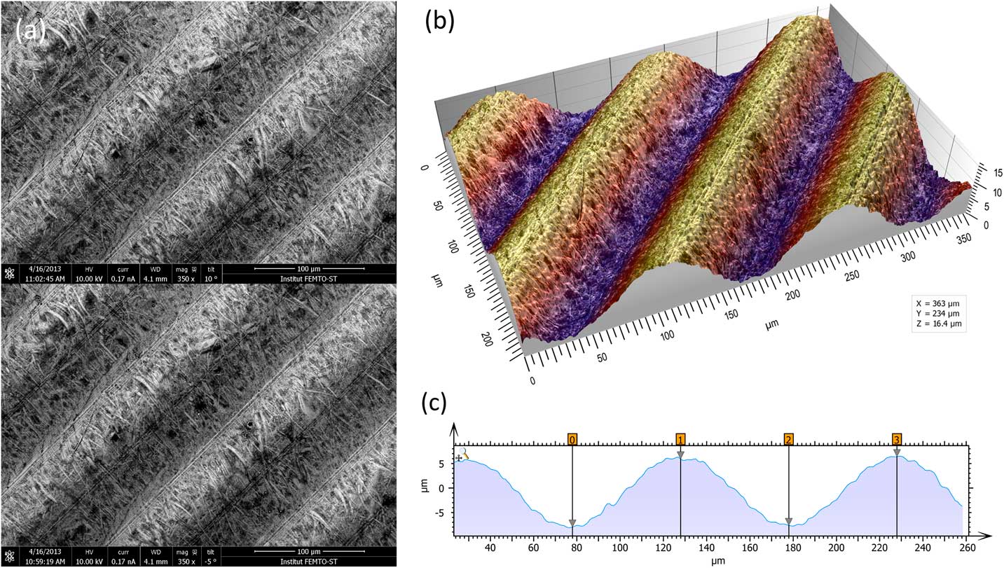
Figure 4 Images of a roughness reference specimen. (a) Two SEM images taken at different angles to the specimen surface. (b) Metrologically accurate topographic reconstruction obtained from the stereo pair, presented in perspective format and colored with a false color shading. (c) Height profile corresponding to a cross section of the 3D topography built by the stereophotogrammetry.
Four-quadrant BSE detectors
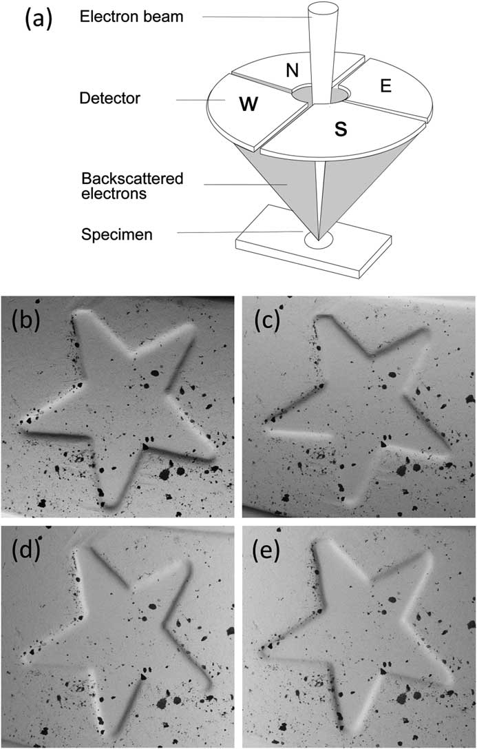
A simpler method for performing reconstruction to reveal the third dimension requires a segmented overhead BSE detector [Reference Pintus5, Reference Paluszynski and Slowko6]. Most such detectors employ four separate sectors symmetrically arranged around a hole for the primary electron beam, but some systems use other arrangements. While MountainsMap SEM can manage various configurations, we will only discuss the four-quadrant case since it is the easiest to understand. A discussion of how this contrast is formed is given in [Reference Goldstein2]. A major advantage of this method is that it only requires taking one “shot” of the sample, since all four images are acquired simultaneously by the four detectors (Figure 5). Each detector pair represents one orthogonal direction (that is, North-South pair and West-East pair). Figures 5b and 5c show images of a euro-coin detail that correspond to the North and South channels of a four-quadrant detector. Holes are difficult to distinguish from black inclusions on the original four images.

Figure 5 A four-quadrant overhead backscatter detector for an SEM. (a) Each detector pair represents one orthogonal direction (i.e., North-South pair and West-East pair). The four detectors produce four different images of the same object. (b) through (e) show a detail on a euro coin in images acquired from the N (b) and S (c) detectors and the W (d) and E (e) detectors. The local slopes at each pixel, ∂z/∂y and ∂z/∂x, can be calculated from the N-S image pair and the W-E image pair, respectively. These calculations are the first step toward producing a height map.
Shape from shading
The shape-from-shading method employs several mathematical steps. First, the slope in the direction of each pair of detectors is calculated (that is, North-South pair and West-East pair). A major advantage of using a pair of detectors symmetrically arranged over the specimen is that the differential signal obtained from the pair neutralizes reflectance and allows the local slope to be calculated. If both signals decrease, we achieve a black dot. Conversely if one signal is high while the other is low, we will obtain a local slope. Each pair of detectors gives, for each pixel, the local slope of the surface z in the pair direction, for example, ∂z/∂x and ∂z/∂y (see Figure 5). This results in two separate scalar fields (that is, two intermediate images of orthogonal derivatives or slopes). Then, the height map z(x,y) is processed by integration of these two local slopes ∂z/∂x and ∂z/∂y. Once the height map is obtained, the height value of each pixel is known, and creation of a 3D representation is just a question of applying 3D rendering algorithms. Relative heights on a surface may be calculated from the differences between the images of each detector pair.
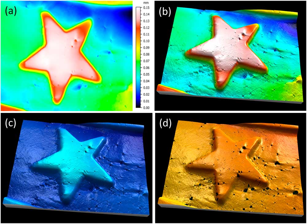
Figure 6 shows images resulting from the following steps. Image (a) is a height map obtained by the integration of slopes. The height is false-color-coded using a lookup table. The rainbow color scale applied here is traditionally used to express height on a physical map, where the lowest points are blue (the sea), the plains are green, the mountains are red, and the highest points are white (snow-capped peaks). Image (b) is the height map used to produce a 3D mesh. At this stage, topography is still shown alone in false color without using the original SEM image for the rendering. Image (c) shows the final 3D rendering. The original SEM image is now pasted onto the previous 3D form to render texture (note that the black inclusions are back, whereas the previous image just shows the pits). Having four different channels allows a different color to be associated with each image pair, resulting in a much clearer perception of surface features. Here purple has been allocated to one pair, and blue to the other, creating a lighting effect on the 3D shape (purple reflections highlight the cliff at the left bottom corner). Image (d) shows the same image, but with yellow and red assigned to the two detector pairs.

Figure 6 Slopes from shading of a detail from a euro coin. Image (a) shows the height map, obtained from the integration of slopes, in the false colors of the rainbow scale. Image (b) shows a 3D mesh derived from the height map. Image (c) shows the 3D mesh combined with the original SEM image. Here purple has been assigned to one pair of detectors and blue assigned to the other. Image (d) shows the same image but with yellow and red allocated to the two pairs of detector signals, producing a brass effect.
Of course, in this type of reconstruction, it is only possible to reconstruct the visible part of the sample (that facing the electron detector). “Cliffs” and overhangs are not taken into account. This method can only be metrologically accurate if all the slopes of the object are visible. Note that unlike conventional stereo imaging (Figure 4), it was not necessary to take two successive scans or to tilt the sample.
Can we get 3D shape from a single SEM image?
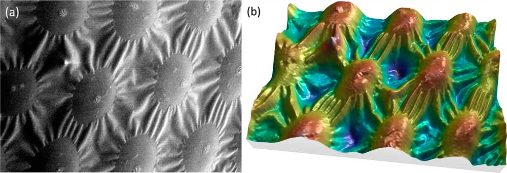
It is commonly accepted that one image alone is not sufficient for producing correct height (Z axis) information. Putting the accuracy of height values aside, however, image reconstruction can provide a useful 3D effect. Under specific conditions, MountainsMap SEM algorithms can produce a credible 3D color model from a single SEM image. While the heights cannot be extracted because the Z axis is not calibrated, the 3D rendering is worth a look (Figure 7). The calculation of this rendering required several steps. First, the image in Figure 7a was subtracted from the least square polynomial of the 2nd degree, that is, a function of type g(x,y) = ax²+ by² + cxy + dx + ey +f, where g(x,y) represents the gray level at the pixel (x,y) and the coefficients a to f give the best fit between g(x,y) and the actual image pixels. This subtraction flattens the global shape of the function without changing the local contrast. Then, since the specimen material here is of a single phase and the surface is lighted from the right side, the gray level can be interpreted as -∂z/∂x (the slope from right to left). Next this slope can be integrated, as for the four-quadrant detector in the previous example, producing a height map. From then on, the process is the same as for Figure 6: a 3D display is generated, and the heights are color-coded using a false-color scale (Figure 7b).

Figure 7 SEM image of spots on a ladybug. (a) Original SEM image exhibiting image noise and a strong shadow effect at the left. Lighting homogeneity was restored by the software before beginning the reconstruction. (b) Same image rendered in 3D, using only the information contained in the first image. Image courtesy of Chris Supranowitz, University of Rochester.
This 3D reconstruction from a single SEM image can only be obtained under certain conditions. The surface of the specimen must be of homogeneous composition and not overly porous. Again, the height values perceived using this technique do not have metrological value, but they may be useful in visual interpretation of the image.
Image segmentation and 3D rendering
It is an advantage and a convenience to be able to work with a single image, particularly with images downloaded from the internet. The “single image reconstruction” operator in MountainsMap uses different methods depending on the image type to produce the 3D rendering, including shape-from-shading integration (ladybug example of Figure 7) and object-oriented segmentation (in Figures 8 and 9).

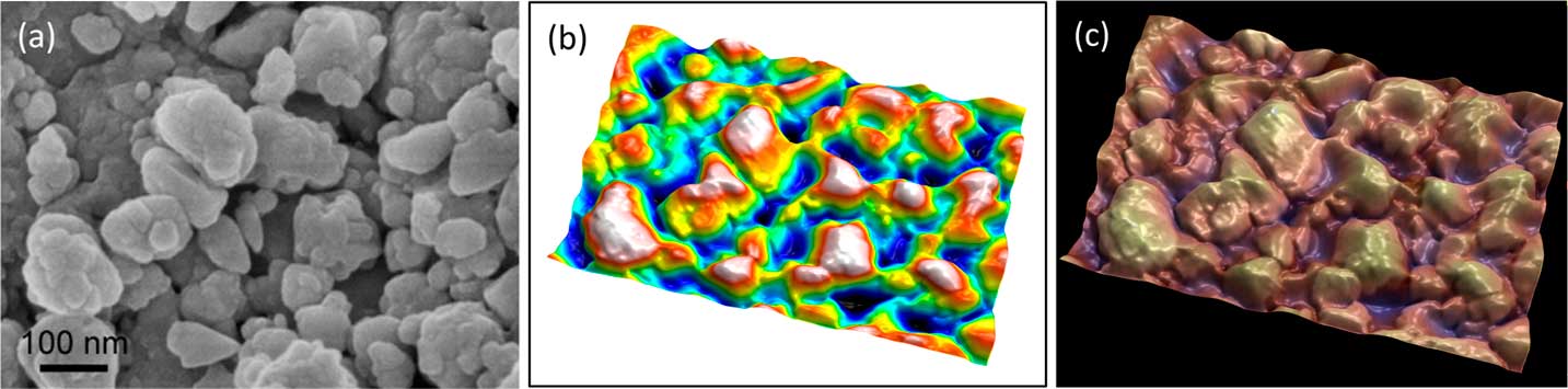
Figure 8 Secondary electron SEM image of lanthanum hexoboride nanoparticles. (a) Original image, (b) height map, and (c) final image. The latter resulted from operation of “single image reconstruction” in MountainMap™ SEM and shows a 3D effect with color rendering. Image courtesy of SkySpring Nanomaterials Inc.
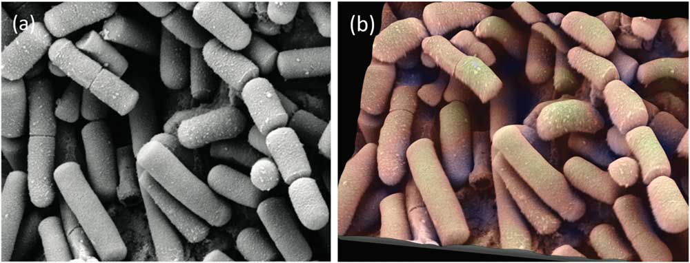
Figure 9 SE SEM image of Bacillus cereus, responsible for some types of food poisoning. (a) Original image from the internet. (b) Same image rendered in 3D with pseudocoloring. Image courtesy of Mogana Das Murtey and Patchamuthu Ramasamy. Licensed under the Creative Commons Attribution-Share Alike 3.0 Unported license, from WikiMedia (https://commons.wikimedia.org/wiki/File:Bacillus_cereus_SEM-cr.jpg).
In Figure 8, object-oriented segmentation was used to separate the objects in the image. This involved a combination of high-pass filtering, a classical watershed algorithm to find object contours, a set of post-processing rules to group or dissociate objects, and some integration to produce a height map. Altogether there are more than 30 operations, but the user is only required to indicate the average size of the objects as a setting. The height map (Figure 8b) can then again be used as a distorted mesh on which the original SEM image is pasted as a texture. Once the height map is obtained, it can also be used to blend a false-color scale with the SEM image as shown in Figure 8c.
Figure 9 shows another image from the internet. Again the single-image reconstruction operator used object-oriented segmentation and 3D rendering to provide both color and shading, giving the image a pleasing and believable 3D-like presentation.
On complex images with multiple object sizes and shapes such as this one, not all objects are reconstructed perfectly in 3D; some might look “deflated.” However, for topography coming from a single SEM image, it is the most one can do so far and allows an easy first approach of the 3D surface. It can be used for instance to compare the relative surface texture properties within a batch of samples or to count objects where classic image segmentation would fail.
Note: Regardless of the colorizing or 3D technique described above, all images in this article were processed using MountainsMap software. Most SEM manufacturers provide software based on MountainsMap with their instruments, as standard or as an option. For more details go to the following: www.digitalsurf.com.
Conclusion
The availability of image enhancement and 3D analysis software for SEM promises to alter image processing practices in science and industry. It crosses an important threshold in allowing researchers to improve visualization and interpretation of objects in the nanoworld through the addition of color and depth. From a practical point of view, the ease of operation frees up precious hours, allowing scientists to spend more time analyzing and applying results rather than producing them.
Acknowledgements
The author would like to thank the many electron microscopists who gave permission for their data to be used in the preparation of this article. Many thanks also to Isabelle Cauwet and Roland Salut who performed sample imaging for Figure 4 within the FEMTO-ST Institute in Besançon, France.


