


Introduction
Rapid prototyping (RP) technology is now taking a prodigious lead in various manufacturing sectors, refining its potential applications on the one hand, while minimizing its limitations on the other hand (Gibson et al., Reference Gibson, Rosen and Stucker2015; Chakrabarti et al., Reference Chakrabarti, Suwas and Arora2022; Khorasani et al., Reference Khorasani, Ghasemi, Rolfe and Gibson2022). The medical industry is a core sector that is highly adaptive to this technique for availing 3D-printed medical equipment, customized splints-orthoses, dental braces, surgical implants, shoe-insoles, neck collars, and even 3D-printed catalytic medicines (Kumar and Chhabra, Reference Kumar and Chhabra2022). The process of RP is technically sound and capable of precisely fabricating any complex geometry; still, it is a reality that printing starts working only when designed 3D models are available (Popescu et al., Reference Popescu, Zapciu, Tarba and Laptoiu2020). Especially when the job is to produce patient-specific orthosis, the geometry of the limb creates a challenging situation for the designer, and thus the utilization of a 3D scanner, concludes the task more effectively and quickly (Farhan et al., Reference Farhan, Wang, Bray, Burns and Cheng2021). In such cases, the reliability of RP becomes highly dependent on optimizing scanning parameters for collecting precise 3D scans (Fitzpatrick et al., Reference Fitzpatrick, Collins and Gibson2020; Kaushik et al., Reference Kaushik, Gahletia, Garg, Sharma, Chhabra and Yadav2022). However, having accurate scans is equally valuable for both subtractive and additive processes for developing precise, appealing, and performance-oriented products.
The accuracy of the 3D scanning approach (3D-SA) is evident in various fields of the medical industry like forensic research, radiology, orthopedics, craniofacial-dentistry, and surgical science, which makes it a strong noninvasive competitor for the scanning utility (Sholts et al., Reference Sholts, Wärmländer, Flores, Miller and Walker2010; Haleem and Javaid, Reference Haleem and Javaid2019; Henson et al., Reference Henson, Constantino, O’Keefe and Popovich2019). Tikuisis et al. (Reference Tikuisis, Meunier and Jubenville2001) performed regression analysis to develop a prediction equation in order to calculate body surface area from the 3D scans. Wang et al. (Reference Wang, Chang and Yuen2003) developed a human model using 3D scanning and a fuzzy logic-based prototype system to preserve the topology scenario of the model. Boehnen and Flynn (Reference Boehnen, Flynn and Stephanie2005) performed a comparative empirical accuracy analysis for different scanning devices to compare their instantaneous point cloud capturing abilities over moving targets. 3D-SA can efficiently measure the burned limb volume in a non-contact manner that is innocuous and recommended for the clinical utility to treat acute burn edema (Edgar et al., Reference Edgar, Day, Briffa, Cole and Wood2008). Toma et al. (Reference Toma, Zhurov, Playle, Ong and Richmond2009) exercised a coordinate-based 3D scanning practice for reproducing clinically acceptable facial landmarks. Telfer and Woodburn (Reference Telfer and Woodburn2010) performed a comparative analysis of the scanning capabilities of various 3D surface scanning techniques in the context of scanning a human foot and the reproducibility of customized utilities like footwear and orthotic products.
The quality of scans delivered by 3D-SA is highly remarkable, and the selection of optimal scanning parameters is somehow extensive. Zaimovic-Uzunovic and Lemes (Reference Zaimovic-Uzunovic and Lemes2010) investigated the influence of an object’s surface color and light intensity over the quality of 3D scanning and found the light gray surfaces as most appropriate for laser scanning. Pesci et al. (Reference Pesci, Teza and Bonali2011) exercised a parametric optimization approach for spatial data acquisition using a terrestrial laser scanner, taking spot spacing and element size as key factors for deciding the acquisition range. To enhance the prosthetic fitting over the residual limb, the accuracy of a 3D scanner was analyzed in terms of cross-sectional area and limb perimeter, resulting in a mean percentage error of less than 2% (Seminati et al., Reference Seminati, Talamas, Young, Twiste, Dhokia and Bilzon2017). The optimization of the scanning plan for 3D-SA, involving a point precision-based level of accuracy and a point density-based level of detail, can smoothly solve the architectural construction problems (Biswas, Reference Biswas2019).
As the quality of 3D scans captured by 3D-SA depends upon numerous factors, still they majorly can be classified into three categories: scanner-specific, surrounding-specific, and target contour-specific (Kaasalainen et al., Reference Kaasalainen, Jaakkola, Kaasalainen, Krooks and Kukko2011; Trebuňa et al., Reference Trebuňa, Mizerák, Trojan and Rosocha2020). One of the most attentively studied factors is light intensity, due to its dynamic nature, which is surrounding specific (Lemeš and Zaimović-Uzunović, Reference Lemeš and Zaimović-Uzunović2009; Amir and Thörnberg, Reference Amir and Thörnberg2017). The capture angle is the second factor which is the object’s contour specific, and the third factor is most cited one in the field that is scanning distance which is scanner specific (Kaasalainen et al., Reference Kaasalainen, Jaakkola, Kaasalainen, Krooks and Kukko2011). It is typical to find the most appropriate combination of scanning parameters over the numerous possibilities to obtain precise results by 3D-SA. The role of artificial intelligence (AI) approaches cannot be neglected when the task is to handle complicated data sets and to predict specific inputs over which optimum results can be achieved (Dhankhar et al., Reference Dhankhar, Kumar, Kumar, Chhabra, Shukla and Gulati2019; Kumar et al., Reference Kumar, Kumar, Chhabra and Shukla2019; Badhwar et al., Reference Badhwar, Kumar, Yadav, Kumar, Siwach, Chhabra and Dubey2020). A considerable impact of the hybrid statistical tools GA-RSM and GA-artificial neural network (ANN) is also evident in predicting the mechanical behavior of 3D printed parts (Deshwal et al., Reference Deshwal, Kumar and Chhabra2020; Kumar et al., Reference Kumar, Gupta and Singh2022); hence, the probability of getting precise results becomes very high if 3D-SA is patched with artificial machine learning statics (Nayak and Das, Reference Nayak, Das, Sezer, Öncü and Boyraz Baykas2020; Voronov and Dovgolevskiy, Reference Voronov and Dovgolevskiy2020).
In this research, three crucial factors (LI, CA and SD) were selected and optimized with the intelligence of artificial hybrid machine learning (AHML) tools to make the 3D-SA more precise and accurate. To enhance the potential abilities of low-cost 3D scanners, an economical portable SENSE 2.0 3D scanner has been used to efficiently and accurately execute wrist scanning under varying conditions. Experimental runs were performed over appropriate combinations of scanning parameters suggested by the CCD matrix to obtain initial/unoptimized results. The accuracy of the scans was analyzed in CREO software through wrist perimeter error (WPE) evaluations over the wrist distal end. The influence of scanning parameters over the WPE and scanning time (ST) was analyzed from the fit statics in RSM and mean square error (MSE) analysis in ANN. Then, the best-fit models corresponding to the high regression values (R) were embedded as fitness functions (FFs) in multi-objective genetic algorithm (MOGA). The execution results of various AHML techniques: RSM, RSMOGA, and MOGA neural networking (MOGANN), were evident in the form of considerable reduction in WPE and ST over the predicted optimal scanning parameters. However, the correlations between predicted and actual values were further validated experimentally, and the results were presented as the reduction in ST and percentage reduction in WPE. The potential of various AHML tools is evident in multiple research sectors for data training, validation and optimization; however, the impact of these tools is not adequately utilized in the context of 3D-SA (Deshwal et al., Reference Deshwal, Kumar and Chhabra2020; Khangwal et al., Reference Khangwal, Chhabra and Shukla2021; Pourmostaghimi et al., Reference Pourmostaghimi, Zadshakoyan, Khalilpourazary and Badamchizadeh2022). The integration of AHML tools with 3D-SA for optimizing various process parameters will enable the collection of highly précised scans in a time-efficient manner and enhance RP’s reliability for the fabrication of customized utility.
Methodology
Pilot runs – Development of CCD matrix
A pilot study was completed to check the specifications of the SENSE 2.0 3D scanner in the clinical environment where direct sunlight is not always possible, intending to refine the range of variables (Table 1) and standardize the entire procedure. Design Expert software was used to generate suitable combinations among the three input variables for scheduling the experimental trials. A CCD matrix (Table 2) was developed based on a randomized multi-level factorial variation approach, providing suitable combinations of input variables for 20 experimental runs. For every input factor, their lower range was added as the value of −alpha and their upper range was added as the value of +alpha by selecting a numeric factor as 3 and a categorical factor as 0, to avoid combinational duplicity in CCD.
Table 1. Ranges of input variables assigned to CCD
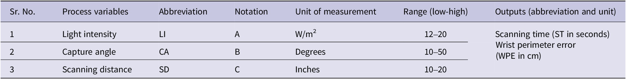
Table 2. Experimental results over the CCD input matrix

Experimental runs
A portable SENSE 2.0 3D scanner was used for scanning the rotating wrist, conveying the point cloud data directly to the SENSE software installed in the laptop through a USB 3.0 cable (Figure 1). To capture the 3D scans, the human wrist (with clenched fist) was considered as the target (as per the requirement of upcoming studies) where the extreme rotational movement of the wrist (non-injured) in a supination-pronation manner aided the scanning of almost 360° views (Figure 1). The wrist was scanned with a clenched fist because the accuracy of the scan is affected and becomes better when the calculation for the fingers is removed from the scan (Edgar et al., Reference Edgar, Day, Briffa, Cole and Wood2008). In order to enhance the scanning, the scanner was kept fixed on a stand over the rotating arm, and the desired angle was set using a clinometer device. To create the light intensity variations (measured by solar power meter KM-SPM-11), the room lighting was changed accordingly and scans were captured from 11 am to 4 pm, which are the regular working hours for a clinic. For every combination of process variables, the scanning process was repeated three times to ensure the repeatability of the process, and the average ST of the three runs was considered as the final value (Table 2).

Figure 1. Experimental setup for scanning human wrist.
Similarly, a total of 60 scanning trials were executed over 20 different parametric combinations. However, for calculating WPE, the accuracy of the wrist perimeter was checked for every scan to obtain the closest value to the actual wrist perimeter, which was 18 cm (on the distal end) in the present study. After completion of each trial, a hollow scan of the concerned geometry was obtained, and every scan was solidified in the SENSE software to obtain the corresponding solid geometry (Figure 2) and saved as a. obj file, for further analysis in CREO Parametric 3.0 M010 (Figure 3).
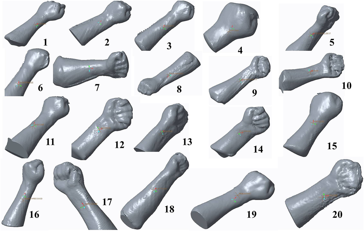
Figure 2. Twenty optimal 3D wrist scans used for X-sectional analysis in CREO.

Figure 3. A systematic multilayer process flowchart for 3D scanning process optimization.
CREO analysis
In CREO, to determine the wrist perimeter of the scanned model over the distal end, a standard procedure was followed. The. obj file was imported by checking the “use template” and “generate log file (short)” dialogue boxes, then a datum axis (F6) was generated by selecting the right (F1) and front (F3) datum planes. Subsequently, a datum plane (F7) was created by selecting F6 and F1 at an offset rotation angle of 338o and further, a datum plane (F8) was created in the reference of F7 at an offset translation (40 to −20; varying as per the variation of capture angle). Finally, a cross section (XSEC001) is created on the distal end using the “view (section-planar)” command in the reference of F8, and then the “model-datum-curve from cross section” command was used to generate a curve (F9) over the XSEC001. Finally, the wrist perimeter of the scanned model over the distal end was measured using the “analysis-measure-length” command in the reference of F9 in the form of curve length. WPE was calculated by subtracting the actual wrist perimeter from the curve length obtained from the CREO analysis, and the procedure was repeated over the 60 scans to get the least WPE among three runs (Table 2) for every 20 parametric combinations.
RSMOGA approach for data evaluation and optimization
RSM creates a regression model “fx” for a chosen experimental design where the value of R2 (regression coefficient) near to 1 and the variances in prediction under a control domain; conclude the quality of the fit.
 $$ \mathrm{PV}=\mathrm{Var}\;\left(\hat{\mathrm{y}}\left(\mathrm{x}\right)\right)={\mathrm{x}}^{\mathrm{m}'}{\left({\mathrm{X}}^{'}\mathrm{X}\right)}^{\hbox{-} 1}{\mathrm{x}}^{\mathrm{m}}{\unicode{x03C3}}^2 $$
Prediction variances (PVs) are calculated as per (1), where ŷ represents the prediction by the model, x represents the point in experimental space, xm’ represents coordinate x expanded in model space, (X’X)−1 is the usual matrix based on the considered factors for analysis, σ2 represents unknown error variance and is targeted to keep the PV as low as much as possible. RSM analysis over the model “fx” provides a separately coded equation for every output that is further fused into the fitness function of the MOGA to activate the optimization process. Despite providing a single optimal result, MOGA provides a set of Pareto-optimal solutions because no solution can be considered better than the other with respect to all objectives. Pareto improvement is an inter-feasible solution movement for making one objective function better without making another one worse and providing a set of Pareto-efficient optimal solutions when no other improvement can be made. Any multi-objective optimization problem can be formulated as, Eq. (2), where fi (x) is the objective function to be minimized, Nobj represents the number of objectives (as Nobj = 2 in the present case), gk (x) and hl (x) are constraints with values of K and L = 0 in the present case.
 $$ {\displaystyle \begin{array}{l}\operatorname{Minimize}\;{f}_i\left(\mathrm{x}\right),i=1\dots \dots ..{N}_{obj}=2;\\ {}\mathrm{Subject}\ \mathrm{to}:{g}_k(x)=0,k=1\dots \dots \dots ..\mathrm{K}\hskip0.35em \&\hskip0.35em {h}_l(x)\le 0,l=1\dots \dots \dots ..\mathrm{L}\end{array}} $$
MOGANN approach for data training and optimization
Both RSM and ANN are used for numerical analysis (data creation-manipulation-fitting-simulation-visualization); however, there is a huge difference in their working. ANN gets its theme from the human nervous system and makes an artificial network for mapping between inputs and targets just like transmitting signals for various sensory inputs in the human nervous system. ANN comprises organized hidden layers of sigmoid neurons (nodes) and output layers of linear neurons, which work like processing units. Each neuron in a layer is connected with every neuron of the preceding layer and enables it to work like a feed-forward data flow network. The mapping performance of ANN is based on the MSE analysis, which calculates the differences between actual values predicted values, and regression analysis, which determines the weightage of input variables over the targets. The five basic equations used in the entire mathematical regression analysis can be understood as follows:
 $$ {e}_j(n)={d}_j(n)-{y}_j(n) $$
For any jth neuron in the output layer at the iteration n, the error term $ {e}_j(n) $
is calculated by subtracting actual output at the jth neuron
$ {e}_j(n) $
is calculated by subtracting actual output at the jth neuron $ {y}_j(n) $
from the desired output at the jth neuron
$ {y}_j(n) $
from the desired output at the jth neuron $ {d}_j(n) $
.
$ {d}_j(n) $
.
 $$ E(n)=\frac{1}{2}\sum_{j\varepsilon C}{E}_j^2(n) $$ $ E(n) $
determines the instantaneous value of error energy at the nth iteration, where j belongs to the set containing all the neurons in the output layer i.e., C.
$ E(n) $
determines the instantaneous value of error energy at the nth iteration, where j belongs to the set containing all the neurons in the output layer i.e., C.
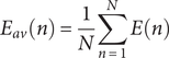 $$ {E}_{av}(n)=\frac{1}{N}\sum_{n=1}^NE(n) $$ $ {E}_{av}(n) $
represents the average square error energy for all the N iterations presented in the network.
$ {E}_{av}(n) $
represents the average square error energy for all the N iterations presented in the network.
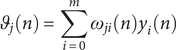 $$ {\vartheta}_j(n)=\sum_{i=0}^m{\omega}_{ji}(n){y}_i(n) $$ $ {\vartheta}_j(n) $
is induced local field at the input of jth neuron, where
$ {\vartheta}_j(n) $
is induced local field at the input of jth neuron, where $ {y}_i(n) $
belongs to the previous layer (hidden) neuron that just precedes the output layer.
$ {y}_i(n) $
belongs to the previous layer (hidden) neuron that just precedes the output layer.
 $$ {y}_j(n)=\varphi\;\left({\vartheta}_j(n)\right) $$
The actual output at the jth neuron $ {y}_j(n) $
is measured as the activation function of
$ {y}_j(n) $
is measured as the activation function of $ {\vartheta}_j(n) $
, where
$ {\vartheta}_j(n) $
, where $ \varphi $
works as an argument of
$ \varphi $
works as an argument of $ {\vartheta}_j(n) $
which modifies all the weighted summations as input to the activation function.
$ {\vartheta}_j(n) $
which modifies all the weighted summations as input to the activation function.
The ANN network continuously moves toward drawing the best. net model for predicting accurate results by assigning suitable weights to the inputs and minimizing the backward propagation error. Like RSMOGA, MOGA further utilizes the weighted model (.net) provided by ANN to align the inputs toward improved outputs.
Result discussion
RSM evaluation-analysis and optimization results
The predicted CCD matrix (20 × 3) of input variables is now patched with experimentally obtained output variable matrix (20 × 2) to proceed further with (20 × 5) input–output matrix for RSM training analysis. RSM advances the evaluation toward the optimization goal using a polynomial model of quadratic order to develop a precise fitting surface by calculating the fraction of design space through 1000 bins (rows) and 15,0000 random points for cuboidal space having radius 1.
During the RSM model evaluation, the value of lack of fit 5 (desirable more than 3) and the value of pure error 5 (desirable more than 4) for the degree of freedom ensures that a valid lack of fit test has been executed. The analysis section of RSM proceeded with “none transformation” as the response range ratio max/min was 1.22299 because transformation is required only when the value is greater than 10. In the fit summary section, cubic model was aliased, while the quadratic versus two-factor interaction model was suggested (p-value ˂ 0.0001) for the accurate fitting of the design. The analysis of variance results for ANOVA (quadratic model) corresponding to ST and WPE (Figures 4 and 5) proved that the model was significant and adequately precise {R2(ST) = 0.9851, R2(WPE) = 0.9873} for the further navigation over unknown inputs through equations (8) and (9).

Figure 4. RSM evaluation and optimization results for WPE (a) ANOVA results, (b) fit statics, (c) coded equation for WPE, and (d) 3D surface plot showing the mutual variation of input factors.

Figure 5. RSM evaluation and optimization results for WPE (a) ANOVA results, (b) fit statics, (c) coded equation for WPE, and (d) 3D surface plot showing the mutual variation of input factors.
The final RSM equation for ST in coded factors:
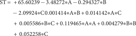 $$ \mathrm{ST}={\displaystyle \begin{array}{l}+65.60239-3.48272\ast \mathrm{A}-0.294327\ast \mathrm{B}\\ {}-\hskip2px 2.09924\ast \mathrm{C}\;0.001414\ast \mathrm{A}\ast \mathrm{B}+0.014142\ast \mathrm{A}\ast \mathrm{C}\\ {}+\hskip2px 0.005586\ast \mathrm{B}\ast \mathrm{C}+0.119465\ast \mathrm{A}\ast \mathrm{A}+0.004279\ast \mathrm{B}\ast \mathrm{B}\\ {}+\hskip2px 0.052258\ast \mathrm{C}\end{array}} $$
The final RSM equation for WPE in coded factors:
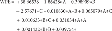 $$ \mathrm{WPE}={\displaystyle \begin{array}{l}+38.66538-1.86428\ast \mathrm{A}-0.398909\ast \mathrm{B}\\ {}-\hskip2px 2.57671\ast \mathrm{C}+0.010830\ast \mathrm{A}\ast \mathrm{B}+0.065079\ast \mathrm{A}\ast \mathrm{C}\\ {}+\hskip2px 0.010633\ast \mathrm{B}\ast \mathrm{C}+0.031034\ast \mathrm{A}\ast \mathrm{A}\\ {}+\hskip2px 0.001432\ast \mathrm{B}\ast \mathrm{B}+0.039754\ast \end{array}} $$
RSM also provides the optimization section for both numerical and graphical analyses. The output factors can be maximized/minimized over a desired range and appropriate weightage. RSM optimization tool provided very useful results over default settings; however, the best results were obtained over the ranges ST (20–22) and WPE (0.5–5.0178). The optimized outputs were recorded as ST = 20.270 sec and WPE = 0.723 cm for the process variables as LI = 13.138, CA = 25.324°, and SD = 17.256 (Figure 6), and it was a notable remark that both factors have been minimized further in comparison with the experimental results.

Figure 6. (a) RSM optimization results and (b) RSMOGA optimization results.
RSMOGA mutual optimization results
The RSM is a sound approach for data fitting and optimization; however, there are still some other valuable options for data optimization, like the MOGA approach. MATLAB was used for the further optimization of the process parameters using MOGA. After starting MATLAB, open the optimization tools from the “app” section and then select MOGA as a problem solver that only works for multiple outputs, as in the present study. It can maximize both outputs or minimize them and simultaneously maximize one while minimizing the other. Before starting the optimization with MOGA, it always requires an FF, a multi-objective vector function that needs to be minimized. FF was designed in the editor window of MATLAB containing all three input variables and both coded equations (8) and (9) of RSM as outputs and saved in the working folder with. mat extension in the form of “@programname,” that is, @mogarsm. MOGA provides various data-specific options to customize the optimization environment according to user requirements. In the present analysis, the number of variables was selected as 3, the lower bound vector was specified as [12 10 10] and the upper bound vector was specified as [20 50 20]. The double vector type population was selected as it is the only option to proceed with constraint-dependent mutation and creation function. The population size was taken as 200, “tournament” as the selection function, crossover fraction as 0.08 for reproduction, crossover function ratio as 1.0, forward migration with fraction 0.2, and interval as 20, stopping criterion as “after the completion of 300 generations” and with some other default options. Finally, the “Pareto front” was selected as a plot function with the value of plot interval as one. The final results were exported to the workspace by selecting the Pareto front index and choosing the “file-export to workspace option”. The “optimresults” file was saved in the working folder to extract the best results from the “x” input variable matrix (18 × 3) and “fval” output variable matrix. After analyzing the results provided by MOGA, the two best combinations, out of 18, were presented in results (Figure 6 and Table 3). However, there was no significant change in the values of ST; however, the WPE was further reduced to 0.252 cm for the process variables as LI = 12.097 W/m2, CA = 23.115°, and SD = 18.899 inch.
MOGANN integrative training-validation-testing and optimization results
In MATLAB, the command “nnstart” actuates the neural curve fitting wizard. To define the fitting problem it is loaded with, inputs as a 3 × 20 matrix (transverse of CCD matrix; set of 20 samples of three inputs) and outputs as a 2 × 20 matrix (having a set of 20 experimental/actual values of two targets). Out of the 100% samples, the supervised training approach uses 70% samples to train and adjust the network for error minimization by assigning random weights. A further 20% were presented to the network as random data that were not utilized earlier during training for network validation and stops further training if a well-generalized network is obtained. The remaining 20% of the samples are presented as a network performance testing data set to evaluate an unbiased performance of the final ANN model without any influence over net training. After the generation of the architecture for fitting network, which comprises two neurons in the output layer preceded by a hidden layer containing 10 neurons, the algorithms start working for network training. Different algorithms have the potential to train the network with respect to training time, memory required for training, level of noise, and population size of a data set; hence, all three were used for obtaining the best-fit model. When the network was trained using Levenberg–Marquardt algorithm (trainalm), value of regression coefficient (R) was obtained as 0.99847 (Table 3), and the value of gradient was reached to its minimum (1.3128e−11) at sixth iteration while the value of MSE was recorded as 0.00788, the value of damping factor (Mu) as 1e−09 (at epoch 6), and the value of best validation performance was recorded as 0.25421 (at epoch 1). Similarly, the network performance was further analyzed over algo-Bayesian Regularization (trainabr) and algo-Scaled Conjugate Gradient (trainascg). After a comparative analysis, the extracted facts concluded that “trainabr” provided the most favorable results: the value of R as 0.99984 (comparatively higher than R(trainalm) = 0.99847 and R(trainascg) = 0.9988), the value of gradient as 0.012767 (at epoch 246), the value of damping factor (Mu) as 5.00e+10 (at epoch 246), and the best training performance as 0.016717 (at epoch 83) as shown in Figure 7. The highest value of R (approaching near 1) for “trainabr” makes it the best candidate for the actuation of the objective function in MOGA, still, the optimization runs were executed corresponding to all three algorithms.
Table 3. Optimization results corresponding to different AHML tools


Figure 7. MOGANN (trainabr) results (a) error histogram, (b) gradient-Mu variation plots, (c) regression plot, (d) performance Plot, and (e) Pareto front plot.
In MOGANN, the final best-fit network (.net file obtained from the ANN) is patched with the FF in MOGA, rather than the coded equation as patched in RSMOGA; however, the rest of the procedure is the same as in RSMOGA. As described earlier, MOGANN provides a set of 18 optimal solutions for every unique FF, corresponding to different algorithms, rather than providing a unique optimal solution. By the comparative study of optimization results, it can be concluded that in comparison with the experimental results, both ST and WPE were further reduced through the implementation of a hybrid MOGANN approach. When talking in the context of time, “trainascg” provided the most favorable result where ST = 18.472 sec; however, when preferred for WPE “trainabr” (with highest R = 0.99984) continued its performance during optimization also and provided not only the best value of WPE = 0.357 cm (minimum ensures the précised scan) but also the one of the most favorable ST = 20.061 sec (lower than as obtained from experimental, RSM and RSMOGA) at the scanning parameters as LI = 12.001 W/m2, CA = 29.428°, and SD = 18.214 inch (Table 3).
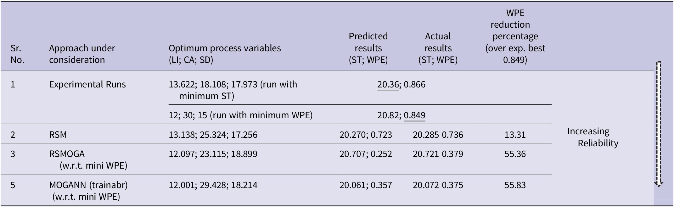
To draw the concluding remarks and to check the repeatability, experimental runs were performed again at the predicted optimum values by different AHML tools, with minimal WPE as a preferred objective, to ensure scanning preciseness and thus reliability of RP for future orthosis going to be made using those scans. During initial experimental runs performed over CCD input variables, the minimum value of WPE obtained was 0.849 cm, which was reduced to its best value of 0.375 cm by MOGANN (trainabr) at the inputs LI = 12.001 W/m2, CA = 29.428°, and SD = 18.214 inch with a WPE reduction percentage of 55.83% (over unoptimized WPE = 0.849), as shown in Table 4. However, the changes in actual ST were not that much different for various approaches; still, it was evident that the least value of ST = 20.072 sec was obtained corresponding to the MOGANN (trainabr) with 1.41% reduction over an unoptimized one, that is, 20.36 sec.
Table 4. Results comparison (predicted v/s actual) for implemented AHML tools
Conclusion
An integrated AHML-3D SA has been successfully developed for availing human wrist scans in reduced time with improved accuracy than that which lacks AI assistance. The tools RSM-RSMOGA-MOGANN were deployed for training between significant input factors and output responses to efficiently optimize ST and WPE over predicted inputs. The results obtained from various AHML tools were compared-validated experimentally and hold a good agreement with the experimental outcomes. The results retrieved from MOGANN (trainabr) have shown maximum convergence, providing a remarkable error reduction of 55.83% in wrist perimeter as WPE is reduced from 0.849 cm to 0.375 cm and a considerable reduction of 1.41% in ST from 20.36 sec to 20.072 sec. The involvement of AHML tools will improve the accuracy of 3D-SA (as error reduction is more than 50%) for capturing precise scans and will enhance the reliability of RP in the arena over conventional manufacturing techniques for developing general as well as user-specific products.
Data availability statement
All data generated or analyzed during this study are included in this published article.
Acknowledgments
The authors sincerely acknowledge Maharshi Dayanand University, Rohtak, India for providing the necessary infrastructure and facilities.
Funding statement
This research has not received any grant from any funding agency.
Competing interest
This is purely a research paper, and it does not include any such kind of information or images for which consent from an individual or institute is required. We also confirm that the manuscript has been read and approved by all named authors and that there are no other persons who satisfied the criteria for authorship but are not listed. We further confirm that the order of the authors listed in the manuscript has been approved by all of us.
Ethics statement
This is an original study and there is nothing unethical.


