


1. Proxy Errors in Capital Estimates
Determining capital requirements accurately for life insurance firms is important both from the perspective of the policyholder and from the perspective of the business. For internal model firms, the Solvency Capital Requirement (SCR) is determined based on a 99.5% value-at-risk (VaR) of assets less liabilities over a one-year periodFootnote 1.
Important risk factors, or variables linked to changes in prices and expected cashflows, are identified, and their joint distribution is estimated. Asset and liability values are considered as functions of these risk factors, and the loss distribution is then defined as the composition of assets less liabilities with the risk factor distribution.
Simple analytic expressions for the loss percentiles are not typically available due to the complexity of the calculation of asset and liability values under risk factor scenarios. In simulation-based capital models, a Monte Carlo approach is used to infer properties of the loss distribution from random samples. It may however be infeasible to compute the large number of simulations required to reduce the Monte Carlo noise to acceptable levels. The underlying calculation complexity may arise from the requirement to process valuations and cashflow projections over a large number of policyholder benefit definitions and assets; complexity may be further compounded when the underlying valuations or cashflow projections are computed with a stochastic model resulting in the well-known problem of nested-stochastics. Hursey et al. (Reference Hursey, Cocke, Hannibal, Jakhria, MacIntyre and Modisett2014) use the term “Heavy models” to refer to calculations required to form the unstressed parts of a firm’s balance sheet.
In this paper, we explore the setting where full Monte Carlo simulation with heavy models is computationally intractable. Alternative approaches must therefore be considered.
Within the life insurance industry, it is common practice to replace the asset and liability functions of risk factors with simpler and faster-to-calculate approximations called proxy models or simply “proxies” (Robinson & Elliott, Reference Robinson and Elliott2014). Androschuck et al. (Reference Androschuck, Gibbs, Katrakis, Lau, Oram, Raddall, Semchyshyn, Stevenson and Waters2017) discuss several approximation techniques that have been motivated by their practical usefulness, including curve fitting, replicating portfolios, and Least Squares Monte Carlo.
Internal model firms are also required to forecast the loss distribution across all percentiles and not only at the 99.5th percentile determining the SCR (ArticleFootnote 2 228.). Proportionality and simplification requirements (Article 56) ensure that firms using simulation-based capital models with proxies accept that the forecasted distribution is approximate and accept that the error may vary across regions of the loss distribution depending on firm’s risk management use cases. For example, the accuracy of proxies in the gain portion of the distribution, or extreme tails, may not affect capital requirements or change use cases, and therefore, a lower accuracy may be acceptable.
Approximation errors do however enter the loss distribution in areas that are both important for capital and other use cases. Outputs of the internal model, including the 99.5th percentile determining the SCR, must be adjusted wherever possible to account for model errors (Article 229(g)). This paper sets out a method that may be used to assess errors propagating into a certain class of percentile estimators and therefore may be directly applicable to actuaries adjusting such model outputs for errors.
The UK’s Prudential Regulation Authority (PRA) reported that firms continue to invest in improving proxy modelling and validation (David Rule, Executive Director of Insurance Supervision, Reference Rule2019):
In May 2018, the PRA issued a survey to a number of life insurers with a proxy model. The responses revealed that over the previous couple of years, some insurers had improved the quality of their proxy modelling considerably. Others had not made the same investment. Standards of validation also varied.
The best firms had increased the number of validation tests by improving the speed of valuation models, were placing the validation tests at points carefully selected to challenge the proxy model calibration and were conducting more validation after the reporting date.
The main challenge in the introduction and use of proxy models is in demonstrating that they reflect the loss distribution and the capital requirements accurately. Androschuck et al. (Reference Androschuck, Gibbs, Katrakis, Lau, Oram, Raddall, Semchyshyn, Stevenson and Waters2017) discuss that this is a design, validation and communication challenge. They highlight the importance of resolving whether fitting errors resulting from the use of proxy models are material and the importance of making suitable adjustments to mitigate the effects of these errors in the capital modelling. The lack of formal proof of the accuracy of quantile estimates was also highlighted:
A proxy model will never replicate a heavy model exactly and so may produce some large errors on particular individual scenarios. However, it can still produce sufficiently accurate quantile estimates as long as individual errors are free from systematic misstatements. Hursey et al. (Reference Hursey, Cocke, Hannibal, Jakhria, MacIntyre and Modisett2014) provided empirical evidence of this; however, the authors of this paper are not aware of a formal proof.Footnote 3
Within this paper, formal proof is given that proxy errors can be removed from the capital estimate in circumstances where, for any given risk factor scenario, proxy errors are within known bounds. This is achieved by a basic analysis of how proxy errors corrupt our knowledge of scenario ordering, allowing the identification of a subset of scenarios that could influence the capital estimate. It is by performing targeted exact computation on the identified subset of scenarios that proxy errors are then eliminated from the capital estimate. The capital estimate remains an estimate due to statistical error, but is devoid of errors arising from the use of proxies. The computational advantage of the approach is measured by comparing the number of targeted scenarios requiring exact calculation to the number of the Monte Carlo scenarios used with the proxy model.
Note that the approach has applicability whenever percentiles of risk distributions are being estimated with proxies. A wide range of actuarial and non-actuarial applications exist where the elimination of proxy errors in quantile estimates may be useful. Applications include the risk assessment of petroleum fields (Schiozer et al., Reference Schiozer, Ligero, Maschio and Risso2008; Risso et al., Reference Risso, Risso and Schiozer2008; Polizel et al., Reference Polizel, Avansi and Schiozer2017; Azad et al., Reference Azad and Chalaturnyk2013) and flood risk modelling (Paquier et al., Reference Paquier, Mignot and Bazin2015). An actuarial example of approximating distributions include Dowd et al. (Reference Dowd, Blake and Cairns2011), where approximations are used to estimate the distribution of annuity values.
The elimination of proxy errors from capital estimates allows actuarial practitioners to state capital requirements as a direct consequence of financial assumptions, model design, and calibrations. Communication of capital requirements may also be simplified when potential errors in the capital estimate, arising from the use of proxies, have been removed.
An important limitation of the approach outlined is that it does not remove the need for validation. Rather, it provides two avenues for practitioners involved in proxy validation. Either the elimination method can be seen as formalising a validation requirement to that of showing an error bound criterion is satisfied, or the method can be used to give insight into the proxy validation process itself by providing a direct linkage between proxy errors and their possible propagation into capital estimates. Full elimination of proxy errors in the capital estimate relies on the proxy error bound being satisfied, and the targeted exact computations being performed.
2. The Proxy Error Elimination Approach
In practice, the underlying loss distributions under consideration are not known analytically and therefore must be studied empirically, in our case, through proxies and Monte Carlo sampling. Our aim is to remove proxy errors from statistical estimates of chosen quantiles, especially the 99.5% value-at-risk corresponding to the Solvency Capital Requirement. Two important questions arise when using proxies to approximate exact losses:
-
How accurate is the quantile estimator when using proxies?
-
Can proxy errors be eliminated from the quantile and standard error estimates?
The elimination of proxy errors from estimates of the standard error is of interest as it may enhance the validation of model stability and may improve evidence of effective statistical processes (Article 124 of European Parliament and of the Council, 2009).
Recall that the proxy loss values for given risk factors are not the actual losses. The actual losses are unknown unless an exact scenario calculation is performed. When using proxies, both the quantile estimator and estimations of its statistical error may deviate from true values due to proxy errors. The elimination of proxy errors relies on the assumption that every loss scenario can be approximated within known error bounds (section 2.5). The error bound may be large or small and may vary by risk factor (Assumption 1). It is through analysis of the upper and lower bounds that important risk factor scenarios are identified. Outside of these the actual proxy may fit poorly but can be ignored since these risk factor scenarios have no impact on the capital estimate.
Under this assumption, it is established that proxy errors can be eliminated from quantile estimators when the losses for a specific set of risk factor scenarios are calculated exactly (Theorem 1). Furthermore, an approximation is proposed for the bootstrap estimation of the standard error which can be calculated without proxy errors when the losses for another set of risk factor scenarios are calculated exactly (section 2.8). To aid understanding of the theoretical statements, an explanatory example with step-by-step calculations is given (section 3).
The results follow from an elementary observation of how the error bounds behave under sorting (Lemma 1). This observation, along with the assumption that proxy error bounds exist, allows the value of the quantile devoid of proxy errors to be known within calculable error bounds (Lemma 2). It is by measuring the possible error within the capital estimate that the error can be shown to be removed.
Without computational restrictions, there would be no need for proxies, and quantiles could be estimated with their standard errors without further approximation error. However, the number of exact loss calculations is in practice restricted (section 2.6). Computational requirements are explored through the consideration of a realistic loss distribution indicating that elimination of proxy errors from capital estimates may be feasible for some firms (section 4).
Initially, notation is set-out to avoid possible confusion between symbols for proxy models and probabilities (section 2.2). The concepts of statistical error and asymptotic convergence are then introduced by looking at the central limit theorem. A family of quantile estimators, called L-estimators, are defined (section 2.3) whose simple linear form plays an important role in the theoretical steps. Estimation of their statistical error is discussed in the context of a technique called the bootstrap (section 2.4) that allows practitioners to estimate statistical errors through resampling of the loss distribution, avoiding the computationally expensive generation of further exact loss scenarios.
2.1 Notational preliminaries
Let the random variable X represent the change in assets less liabilities over a one-year horizonFootnote 4. Negative values of X will represent losses and positive values will represent gains. The 1 in 200 loss is given by the 0.5th percentile of the distribution. The capital requirement is the amount required to be held by the firm to cover this potential loss.
The internal model associates a given risk factor $r\in\mathbb{R}^m$
with a loss
$r\in\mathbb{R}^m$
with a loss $x(r)\in\mathbb{R}$
. We call x(r) the exact loss calculation since it contains no proxy error. The risk factor is considered as a random variable, denoted R, distributed according to a known multivariate distribution, so that the loss X satisfies the composition relationship:
$x(r)\in\mathbb{R}$
. We call x(r) the exact loss calculation since it contains no proxy error. The risk factor is considered as a random variable, denoted R, distributed according to a known multivariate distribution, so that the loss X satisfies the composition relationship:
 \begin{equation}X \sim x(R).\end{equation}
Here the notation $A\sim B$
means A and B have equal distribution. A proxy function for x is a function p of the risk factor space that is inexpensive to evaluate. Where lower and upper error bounds on the exact loss are known, they can be considered as functions of the risk factor space satisfying:
$A\sim B$
means A and B have equal distribution. A proxy function for x is a function p of the risk factor space that is inexpensive to evaluate. Where lower and upper error bounds on the exact loss are known, they can be considered as functions of the risk factor space satisfying:
 \begin{equation}l(r) \leq x(r) \leq u(r).\end{equation}
The distribution function of X is denoted by F and its density function by f, if it exists, so that
 \begin{equation}F(s) = \mathbb{P}(X\leq s) = \int_{-\infty}^{s} f(t)\,\mathrm{d}t, \quad -\infty < s < \infty.\end{equation}
The function F is called the loss distribution. For a given percentile $\alpha\in(0,1)$
, the quantile
$\alpha\in(0,1)$
, the quantile $\xi_{\alpha}$
of the loss distribution is defined by the generalised inverse of F:
$\xi_{\alpha}$
of the loss distribution is defined by the generalised inverse of F:
 \begin{equation}\xi_{\alpha} = F^{-1}(\alpha) \,:\!=\, \inf\{s : F(s)\geq \alpha\},\quad 0 < \alpha <1.\end{equation}
To avoid notational confusion, note that the symbol p is used only to refer to the proxy, whereas probability percentiles are given the symbol $\alpha$
.
$\alpha$
.
The capital requirement is defined as the one in two hundred loss given by $-\xi_{0.005}$
. Note that a minus sign has been introduced so that the capital requirement is stated as a positive number. The value
$-\xi_{0.005}$
. Note that a minus sign has been introduced so that the capital requirement is stated as a positive number. The value $\xi_{\alpha}$
is not easily calculable since f and F are not known precisely. Estimation techniques are therefore required. In the following, statistical estimation techniques involving Monte Carlo sampling are introduced.
$\xi_{\alpha}$
is not easily calculable since f and F are not known precisely. Estimation techniques are therefore required. In the following, statistical estimation techniques involving Monte Carlo sampling are introduced.
2.2 Basic estimation
Distributional parameters of a random variable can be estimated from empirical samples. Estimators can target parameters such as the mean, variance, and quantiles. They are designed to converge to the parameter’s value as the sample size is taken ever larger. Moreover, it is a common phenomenon that the distribution of the error between the estimator and the parameter, when suitably scaled, converges towards normal for large sample sizesFootnote 5. An elementary example of this is the central limit theorem (Chapter 8 of Stirzaker, Reference Stirzaker2003) where under mild conditions on the independent identically distributed random variables $X_i$
with mean
$X_i$
with mean $\mu$
and variance
$\mu$
and variance $\sigma^2$
:
$\sigma^2$
:
 \begin{equation}\mathbb{P}\left( \frac{1}{\sigma \sqrt{n}}\sum_{i=1}^n (X_i-\mu) \leq s\right) \rightarrow \Phi(s) \,:\!=\, \int_{-\infty}^s \frac{1}{\sqrt{2\pi}}e^{-\frac{1}{2}t^2}\,\mathrm{d}t,\quad \text{as }n\rightarrow \infty.\end{equation}
Equivalently, it may be said that the error between the estimator $n^{-1}\sum_{i=1}^n X_i$
and parameter
$n^{-1}\sum_{i=1}^n X_i$
and parameter $\mu$
is approximately normal and, when suitably scaled, converges in distributionFootnote 6, written
$\mu$
is approximately normal and, when suitably scaled, converges in distributionFootnote 6, written
 \begin{equation}\sqrt{n}\left( \frac{1}{n}\sum_{i=1}^n X_i\,\,-\mu \right)\xrightarrow{d} N\left(0,{\sigma^2}\right),\quad\text{as }n\rightarrow\infty.\end{equation}
When the distribution of the estimator (suitably scaled) converges to normal, it is said that the estimator is asymptotically normal. The difference between the estimator and the parameter is called statistical error. The standard deviation of the statistical error is called the standard errorFootnote 7. We discuss the estimation of statistical error in section 2.4. These quantities are of interest since they allow for the construction of confidence intervals for the parameter.
For a given sample size n, the kth largest sample is called the kth order statistic. Given n independent identically distributed random variables $X_i$
, the kth largest is denoted by
$X_i$
, the kth largest is denoted by $X_{k:n}$
. Order statistics are important for our framework since they are very closely related to the quantiles of the distribution. A simple case of asymptotic normality of order statistics is given by Corollary B, section 2.3.3 of Serfling (Reference Serfling2009), where it is shown that if F possesses a positive density f in a neighbourhood of
$X_{k:n}$
. Order statistics are important for our framework since they are very closely related to the quantiles of the distribution. A simple case of asymptotic normality of order statistics is given by Corollary B, section 2.3.3 of Serfling (Reference Serfling2009), where it is shown that if F possesses a positive density f in a neighbourhood of $\xi_{\alpha}$
, and f is continuous at
$\xi_{\alpha}$
, and f is continuous at $\xi_{\alpha}$
, then
$\xi_{\alpha}$
, then
 \begin{equation}\sqrt{n}\left( X_{\lceil \alpha n\rceil:n}-\xi_{\alpha}\right) \xrightarrow{d} N\left(0,\frac{\alpha(1-\alpha)}{f^2(\xi_{\alpha})} \right), \quad\text{as }n\rightarrow\infty.\end{equation}
Estimators taking the form of a weighted sum of ordinals are referred to as L-estimatorsFootnote 8 and can be written
 \begin{equation}T_n = \sum_{i=1}^n c_iX_{i:n}\end{equation}
where $c_i$
are constants dependent on the percentile
$c_i$
are constants dependent on the percentile $\alpha$
and the number of scenarios n and vary according to the chosen estimator. Depending on the choice of weights, L-estimators can target different parameters of the distribution. An elementary example of estimating the mean
$\alpha$
and the number of scenarios n and vary according to the chosen estimator. Depending on the choice of weights, L-estimators can target different parameters of the distribution. An elementary example of estimating the mean $\mu$
of X. By placing
$\mu$
of X. By placing $c_i=1/n$
in (8) and applying (6), noting that the sum of the ordinals is equal to the sum of the sample, we have
$c_i=1/n$
in (8) and applying (6), noting that the sum of the ordinals is equal to the sum of the sample, we have $\sqrt{n}\left(T_n-\mu\right) \xrightarrow{d} N(0,\sigma^2)$
.
$\sqrt{n}\left(T_n-\mu\right) \xrightarrow{d} N(0,\sigma^2)$
.
When the underlying distribution of X is known, the distribution and density functions of $X_{k:n}$
can be derived through elementary probabilityFootnote 9:
$X_{k:n}$
can be derived through elementary probabilityFootnote 9:
 \begin{equation}F_{X_{k:n}}(s) = \sum_{i=k}^n \left(\begin{array}{l}n\\i\end{array}\right) F(s)^i(1-F(s))^{n-i}, \quad -\infty < s< \infty, \end{equation}
 \begin{equation} f_{X_{k:n}}(s) = \frac{n!}{(n-k)!(k-1)!} f(s)F(s)^{k-1}(1-F(s))^{n-k}.\end{equation}
The expected value of the kth order statistic is given by
 \begin{equation}\mathbb{E}\left[X_{k:n}\right] = \frac{1}{B(k,n-k-1)}\int_0^1 F^{-1}(t)t^{k-1}(1-t)^{n-k}\,\mathrm{d}t\end{equation}
where B(x,y) is defined in (16c).
Next we consider a special case of L-estimators designed to target quantiles. This is of particular interest since capital requirements are determined by quantile estimates.
2.3 Quantile L-estimators
In our application, we are concerned with the special case of L-estimators that target quantiles $\xi_{\alpha}$
, and importantly the special case of
$\xi_{\alpha}$
, and importantly the special case of $\alpha=0.005$
representing the 1 in 200 year loss. We call these quantile L-estimators and write their general form as
$\alpha=0.005$
representing the 1 in 200 year loss. We call these quantile L-estimators and write their general form as
 \begin{equation}\hat{\xi}_{\alpha} = \sum_{i=1}^n c_iX_{i:n}\end{equation}
where we use the hat notation $\hat{\xi}_{\alpha}$
to highlight that the estimator is targeting
$\hat{\xi}_{\alpha}$
to highlight that the estimator is targeting $\xi_{\alpha}$
. For a given empirical sample
$\xi_{\alpha}$
. For a given empirical sample $\{x_i\}_{i=1}^N$
from x(R), write the ordered values by
$\{x_i\}_{i=1}^N$
from x(R), write the ordered values by $\{x_{(i)}\}_{i=1}^N$
so that
$\{x_{(i)}\}_{i=1}^N$
so that $x_{(i)}\leq x_{(i+1)}$
for
$x_{(i)}\leq x_{(i+1)}$
for $i=1,\ldots,N-1$
and the value of the statistic for the sample is written
$i=1,\ldots,N-1$
and the value of the statistic for the sample is written $\sum_{i=1}^n c_ix_{(i)}$
.
$\sum_{i=1}^n c_ix_{(i)}$
.
We give here two basic examples of quantile L-estimators. In practice, the choice of the estimator involves considerations of bias and variance, as well as the number of non-zero weights involved in its calculation.
2.3.1 Basic L-estimator
To understand the form of quantile L-estimators, consider a basic example where the quantile is approximated by a single order statistic:
 \begin{equation}\hat{\xi}_{\alpha} = X_{\lceil \alpha n \rceil:n}.\end{equation}
This can be seen as having the form of the L-estimator (12) by setting
 \begin{equation}c_i = \delta_{i,\lceil \alpha n\rceil}, \end{equation}
where $\delta_{i,j}$
is the Kronecker delta notation satisfying
$\delta_{i,j}$
is the Kronecker delta notation satisfying $\delta_{i,j}=0$
whenever
$\delta_{i,j}=0$
whenever $i\neq j$
and
$i\neq j$
and $\delta_{i,i}=1$
. From (7), we see that under mild assumptions the estimator converges to the quantile with asymptotically normal statistical error:
$\delta_{i,i}=1$
. From (7), we see that under mild assumptions the estimator converges to the quantile with asymptotically normal statistical error:
 \begin{equation}\sqrt{n}\left(\hat{\xi}_{\alpha} - \xi_{\alpha}\right) \xrightarrow{d} N\left(0, \frac{\alpha(1-\alpha)}{f^2(\xi_{\alpha})}\right)\quad \text{as }n\rightarrow\infty.\end{equation}
One reason to use the basic estimator is its simplicity. However, estimators with lower standard error may be preferred. An example is the following.
2.3.2 Harrell-Davis L-estimator
Harrell & Davis (Reference Harrell and Davis1982) introduced the quantile estimator that weights ordinals according to the target percentile $\alpha$
in a neighbourhood around the
$\alpha$
in a neighbourhood around the $n\alpha$
-th ordinal. It is given by
$n\alpha$
-th ordinal. It is given by
 \begin{equation}\hat{\xi}_{\alpha} = \sum_{i=1}^n w_{i}X_{i:n}\end{equation}
with coefficients $w_{i}$
dependent on n and
$w_{i}$
dependent on n and $\alpha$
given by
$\alpha$
given by
 \begin{equation}w_{i} = I_{i/n}(\alpha(n+1),(n+1)(1-\alpha)) - I_{(i-1)/n}(\alpha(n+1),(n+1)(1-\alpha))\end{equation}
where $I_x(a,b)$
denotes the incomplete-Beta function
$I_x(a,b)$
denotes the incomplete-Beta function
 \begin{equation}I_x(a,b) = \frac{B(x;\,a,b)}{B(1;\, a,b)}, \quad B(x;\, a,b) = \int_0^x t^{a-1}(1-t)^{b-1} \mathrm{d}t, \quad x>0\end{equation}
formed from the Beta function $B(x;\, a,b)$
. When
$B(x;\, a,b)$
. When $x=1$
, write
$x=1$
, write $B(x,y)\equiv B(1;\,x,y)$
.
$B(x,y)\equiv B(1;\,x,y)$
.
Asymptotic normality of the Harrell-Davis estimator was established by Falk (Reference Falk1985) under general conditions on the distribution involving smoothness of F and positivity of f. A rate of convergence was also derived under somewhat stronger conditions. Numerical properties of the estimator were investigated by Harrell & Davis (Reference Harrell and Davis1982).
2.4 Bootstrap estimation of statistical error
Estimators with low statistical errors are desirable due to them yielding small statistical error bounds on capital estimates. In section 2.3.1, it is shown that in the case of the estimator using a single order statistic, the standard error is approximately $\sqrt{\frac{\alpha(1-\alpha)}{nf^2(\xi_{\alpha})}}$
. This analytic expression for the standard error requires knowledge of
$\sqrt{\frac{\alpha(1-\alpha)}{nf^2(\xi_{\alpha})}}$
. This analytic expression for the standard error requires knowledge of $f(\xi_{\alpha})$
, the density of the loss distribution at the quantile
$f(\xi_{\alpha})$
, the density of the loss distribution at the quantile $\xi_{\alpha}$
. In practical examples, f is not known analytically at any quantile. We therefore need a method of approximating the statistical error of estimators.
$\xi_{\alpha}$
. In practical examples, f is not known analytically at any quantile. We therefore need a method of approximating the statistical error of estimators.
Efron (Reference Efron1979) introduced a technique called the bootstrapFootnote 10 that can be used in practical situations to investigate the distribution of statistical errors when sampling from unknown distributions. This allows, for example, the standard error to be approximated, for example, the parameter $\sigma$
in (6), and the expression
$\sigma$
in (6), and the expression $\sqrt{\frac{\alpha(1-\alpha)}{nf^2(\xi_{\alpha})}}$
in (15).
$\sqrt{\frac{\alpha(1-\alpha)}{nf^2(\xi_{\alpha})}}$
in (15).
Suppose there is a sample $\{x_i\}_{i=1}^n$
from an unknown distribution F. A statistic, say
$\{x_i\}_{i=1}^n$
from an unknown distribution F. A statistic, say $\hat{\xi}_{\alpha}$
, has been calculated on the basis of the sample, and the question is how representative is it of
$\hat{\xi}_{\alpha}$
, has been calculated on the basis of the sample, and the question is how representative is it of $\xi_{\alpha}$
?
$\xi_{\alpha}$
?
Calculating many such samples from F to analyse statistical errors may be prohibitively expensive or even not possible in real-life empirical settings. The bootstrap technique instead uses resampling with replacement to mimic new independent samples. The technique involves drawing an independent sample of size n from $\{x_i\}_{i=1}^n$
with replacement, denoted with star notation
$\{x_i\}_{i=1}^n$
with replacement, denoted with star notation $\left\{x_i^*\right\}_{i=1}^n$
. Resampling from
$\left\{x_i^*\right\}_{i=1}^n$
. Resampling from $\{x_i\}_{i=1}^n$
is computationally cheap and so this can be repeated many times. Each of our new samples gives a realisation of the estimator
$\{x_i\}_{i=1}^n$
is computationally cheap and so this can be repeated many times. Each of our new samples gives a realisation of the estimator $\hat{\xi}_{\alpha}^*$
, and we combine these to form an empirical distribution, from which the variance (and other properties) can be estimated. In applications, the bootstrap variance
$\hat{\xi}_{\alpha}^*$
, and we combine these to form an empirical distribution, from which the variance (and other properties) can be estimated. In applications, the bootstrap variance $\mathrm{var}\left(\hat{\xi}_{\alpha}^*\right)$
is often considered an estimator for the original variance
$\mathrm{var}\left(\hat{\xi}_{\alpha}^*\right)$
is often considered an estimator for the original variance $\mathrm{var}(\hat{\xi}_{\alpha})$
.
$\mathrm{var}(\hat{\xi}_{\alpha})$
.
An algorithm for calculating the bootstrap estimate of standard errors in described in Algorithm 6.1 of Efron & Tibshirani (Reference Efron and Tibshirani1994). Analytical expressions for the bootstrap sample means, variances and covariances were established by Hutson & Ernst (Reference Hutson and Ernst2000). They show that the bootstrap sample is equivalent to generating a random sample of size n drawn from the uniform distribution U(0,1) with order statistics $(U_{1:n},\ldots,U_{n:n})$
and applying the sample quantile function
$(U_{1:n},\ldots,U_{n:n})$
and applying the sample quantile function $F_n^{-1}$
defined by
$F_n^{-1}$
defined by
 \begin{equation}F_n^{-1}(u) = x_{(k)}\quad\text{where } (k-1)/n < u \leq k/n, k\in\mathbb{N}.\end{equation}
Denote the mean and variance of the ordinal $X_{k:n}$
by
$X_{k:n}$
by $\mu_k$
and
$\mu_k$
and $\sigma_k$
respectively, so that
$\sigma_k$
respectively, so that
 \begin{equation}\mu_k = \mathbb{E}(X_{k:n}), \end{equation}
 \begin{equation}\sigma_k^{2} = \mathrm{var}\left(X_{k:n}\right).\end{equation}
Theorem 1 of Hutson & Ernst (Reference Hutson and Ernst2000) establishes that the bootstrap estimators of $\mu_k$
and
$\mu_k$
and $\sigma_k$
denoted
$\sigma_k$
denoted $\mu_k^*$
and
$\mu_k^*$
and $\sigma_k^*$
are given by
$\sigma_k^*$
are given by
 \begin{equation}\mu_k^* = \mathbb{E}\left(F_n^{-1}\left(U_{k:n}\right)\right) = \sum_{i=1}^n w_i(k)x_{(i)}, \text{where} \end{equation}
 \begin{equation}w_i(k) \,:\!=\, I_{i/n}(k, n-k+1) - I_{(i-1)/n}(k, n-k+1), \end{equation}
and $I_x(a,b)$
denotes the incomplete-Beta function defined in (16c). From (10) and the form of
$I_x(a,b)$
denotes the incomplete-Beta function defined in (16c). From (10) and the form of $F_n$
, we see that when
$F_n$
, we see that when $\alpha(n+1)=k$
, the Harrell-Davis weights
$\alpha(n+1)=k$
, the Harrell-Davis weights $w_i$
, defined in (16b), exactly coincide with the bootstrap weights
$w_i$
, defined in (16b), exactly coincide with the bootstrap weights $w_i(k)$
defined in (20b).
$w_i(k)$
defined in (20b).
The bootstrap variance $\sigma_k^{*2}$
is established in Theorem 2 of Hutson & Ernst (Reference Hutson and Ernst2000):
$\sigma_k^{*2}$
is established in Theorem 2 of Hutson & Ernst (Reference Hutson and Ernst2000):
 \begin{equation}\sigma_k^{*2} \,:\!=\, \mathrm{var}\left(F_n^{-1}\left(U_{k:n}\right)\right) = \sum_{i=1}^n w_i(k)\left(x_{(i)} - \mu_k^*\right)^2\end{equation}
where $w_i(k)$
is given by (20b).
$w_i(k)$
is given by (20b).
An interpretation of (2.4) is that for a given loss scenario, the relative chance (in the sense of the bootstrap) amongst all ordinals that the i-th ordinal represents the true quantile ( $\alpha=k/n)$
is given by the weight
$\alpha=k/n)$
is given by the weight $w_i$
.
$w_i$
.
2.5 Assumption on proxy errors
The term proxy error refers to approximations introduced by the use of proxies. For a given risk factor scenario r, we denote the output of a proxy model by p(r) and the exact loss calculation x(r). Fundamental to our analysis is the following assumption regarding knowledge of proxy error bounds.
Assumption 1. The proxy model is calculated with known proxy error bounds: given a risk factor scenario r, the (possibly unknown) exact loss scenario x(r) satisfies
 \begin{equation}l(r) \leq x(r) \leq u(r)\end{equation}
for some known values l(r),u(r).
In practical applications, Assumption 1 can be satisfied by choosing prudent error bounds, as may be found as part of the design and validation of the proxy model. Proxy design within life insurance capital applications is discussed in Caroll & Hursey (Reference Caroll and Hursey2011), Hursey (Reference Hursey2012), and Hursey et al. (Reference Hursey, Cocke, Hannibal, Jakhria, MacIntyre and Modisett2014). Androschuck et al. (Reference Androschuck, Gibbs, Katrakis, Lau, Oram, Raddall, Semchyshyn, Stevenson and Waters2017) suggest during design and validation to consider, amongst other measures, the maximum absolute error amongst in and out-of-sample testing across the whole distribution. Under this approach, prudent choices of error bounds are larger than the maximum error observed.
For a given sample of risk factors $\{r_i\}_{i=1}^n$
, the associated error sample, also called the residuals, is given by
$\{r_i\}_{i=1}^n$
, the associated error sample, also called the residuals, is given by $\{p(r_i)-x(r_i)\}_{i=1}^n$
. The residuals may also be considered as a random sample from
$\{p(r_i)-x(r_i)\}_{i=1}^n$
. The residuals may also be considered as a random sample from $p(R)-x(R)$
. The case when the error is bounded is covered by our framework. Suppose the residual, considered as a random variable, is bounded by some
$p(R)-x(R)$
. The case when the error is bounded is covered by our framework. Suppose the residual, considered as a random variable, is bounded by some $\Delta>0$
:
$\Delta>0$
:
 \begin{equation}p(R) - x(R) \sim E, \quad |E|\leq \Delta.\end{equation}
Then by placing $l(r)=p(r)-\Delta$
and
$l(r)=p(r)-\Delta$
and $u(r)=p(r)+\Delta$
, the conditions of Assumption 1 are satisfied.
$u(r)=p(r)+\Delta$
, the conditions of Assumption 1 are satisfied.
Assumption 1 asserts no distributional properties on the error sample other than that the residuals are bounded for a given risk factor by known values. Assumption 1 is also trivially satisfied in the situation where a proxy function p has a constant error bound $\Delta>0$
so that
$\Delta>0$
so that
 \begin{equation}p(r)-\Delta \leq x(r) \leq p(r) + \Delta.\end{equation}
Similar to case (23), this can be seen by setting $l(r)=p(r)-\Delta$
and
$l(r)=p(r)-\Delta$
and $u(r)=p(r)+\Delta$
. Assumption 1 is however much more general since it allows the error interval to be arbitrarily large and to vary with risk factor.
$u(r)=p(r)+\Delta$
. Assumption 1 is however much more general since it allows the error interval to be arbitrarily large and to vary with risk factor.
Hursey et al. (Reference Hursey, Cocke, Hannibal, Jakhria, MacIntyre and Modisett2014) describe an error function, formed from fitting a function from the risk factor space to the residuals, to inform the design of the proxy function. This error curve cannot be used directly to form upper and lower error bounds since it is formed from least-squares fitting, and therefore represents an averaged error. However, Cardiel (Reference Cardiel2009) shows how least-squared fitting can be adapted to create regressions of the upper and lower boundaries of data sets. In this application, a regression of the upper boundary of the residuals could be used to propose an upper bound function u(r). Similarly, a regression of the lower boundary of the residuals can be used to propose a lower bound function l(r).
Whatever technique is used to pose error bound functions, it is still necessary to appropriately validate the functions before use in capital requirement modelling.
In the analysis of Murphy & Radun (Reference Murphy and Radun2021), an assumption that the error term is normally distributed is made so that
 \begin{equation}p(R) - x(R) \sim N(\mu, \sigma), \quad \mu\in\mathbb{R},\sigma>0.\end{equation}
This setting is excluded from our framework since it is not possible to assert any finite lower and upper bounds on the proxy error, and therefore requirement (22) of Assumption 1 is not satisfied. We note that deconvolution techniques may be applicable when an unbounded error model is assumed; see for example Ghatak & Roy (Reference Ghatak and Roy2018).
2.6 Assumptions on computational feasibility
Practical computational considerations motivate the use of approximation methods in capital requirement modelling. To reflect this, computational restrictions are introduced into the framework. By doing so, practical limitations faced by firms on the volume of computations they can perform are captured. Such limitations may arise for example through time constraints, computational budgets or practical considerations arising from the use of third party systems.
Assumption 2. The following are feasible computations for n, N where $n\ll N$
:
$n\ll N$
:
-
(1) creation of a large number of independent risk factor samples $\{r_i\}_{i=1}^N$
,
$\{r_i\}_{i=1}^N$
, -
(2) evaluation of the proxy, and lower and upper proxy error bounds on a large number of risk factor scenarios
$\{p(r_i)\}_{i=1}^N,\{l(r_i)\}_{i=1}^N,\{u(r_i)\}_{i=1}^N$
, and -
(3) calculation of exact losses for a small risk factor scenario set represented by
$\{x(r_i)\}_{i=1}^n$
.


It is infeasible to evaluate the exact losses for all the risk factor scenarios $\{x(r_i)\}_{i=1}^N$
.
$\{x(r_i)\}_{i=1}^N$
.
The notation $n\ll N$
is used to mean that N may be several orders of magnitude bigger than n. Androschuck et al. (Reference Androschuck, Gibbs, Katrakis, Lau, Oram, Raddall, Semchyshyn, Stevenson and Waters2017) cite a 2014 survey by Deloitte showing life insurance firms using between 20 and 1,000 exact loss calculations for calibration purposes. From this, we infer the likely number of feasible exact computations n for UK based life insurance firms to be at least in the range 20–1,000 and likely much higher given advances in computing capacity since 2014. They also state that to create a credible distribution of profit and loss, firms would expect to run hundreds of thousands, or even millions of scenarios, leading us to infer that N is of the order of one million. For our exposition, we consider
$n\ll N$
is used to mean that N may be several orders of magnitude bigger than n. Androschuck et al. (Reference Androschuck, Gibbs, Katrakis, Lau, Oram, Raddall, Semchyshyn, Stevenson and Waters2017) cite a 2014 survey by Deloitte showing life insurance firms using between 20 and 1,000 exact loss calculations for calibration purposes. From this, we infer the likely number of feasible exact computations n for UK based life insurance firms to be at least in the range 20–1,000 and likely much higher given advances in computing capacity since 2014. They also state that to create a credible distribution of profit and loss, firms would expect to run hundreds of thousands, or even millions of scenarios, leading us to infer that N is of the order of one million. For our exposition, we consider $n=1,000$
and
$n=1,000$
and $N=1,000,000$
to be realistic values for some firms. Firms interested in understanding how proxy errors enter their capital estimates can adjust error bounds, n and N to their circumstances.
$N=1,000,000$
to be realistic values for some firms. Firms interested in understanding how proxy errors enter their capital estimates can adjust error bounds, n and N to their circumstances.
A consequence of Assumption 2 is that the residual error sets of the form $\{p(r_i)-x(r_i)\}_{i=1}^m$
, considered in section 2.5, are feasible to compute for
$\{p(r_i)-x(r_i)\}_{i=1}^m$
, considered in section 2.5, are feasible to compute for $m=n$
but infeasible for
$m=n$
but infeasible for $m=N$
.
$m=N$
.
Next, we consider the construction of computationally feasible bounds on quantile L-estimators.
2.7 Estimating quantiles of the loss distribution
Our interest is to estimate a quantile $\xi_{\alpha}$
, and especially
$\xi_{\alpha}$
, and especially $\xi_{0.005}$
, of the loss distribution without the presence of proxy errors. With a lemma about ordered sequences, we will apply quantile L-estimators to computable quantities to create lower and upper bounds on the L-estimator.
$\xi_{0.005}$
, of the loss distribution without the presence of proxy errors. With a lemma about ordered sequences, we will apply quantile L-estimators to computable quantities to create lower and upper bounds on the L-estimator.
Lemma 1. Let $\{a_i\}_{i=1}^N\subset\mathbb{R}$
and
$\{a_i\}_{i=1}^N\subset\mathbb{R}$
and $\{b_i\}_{i=1}^N\subset\mathbb{R}$
be arbitrary and unordered sequences of real numbers of length N satisfying the component-wise inequality:
$\{b_i\}_{i=1}^N\subset\mathbb{R}$
be arbitrary and unordered sequences of real numbers of length N satisfying the component-wise inequality:
 \begin{equation} a_i\leq b_i\quad \text{for}\quad i=1,\ldots,N. \end{equation}
Denote the ordered sequences by $\{a_{(i)}\}_{i=1}^N$
and
$\{a_{(i)}\}_{i=1}^N$
and $\{b_{(i)}\}_{i=1}^N$
so that
$\{b_{(i)}\}_{i=1}^N$
so that $a_{(i)}\leq a_{(i+1)}$
and
$a_{(i)}\leq a_{(i+1)}$
and $b_{(i)}\leq b_{(i+1)}$
for
$b_{(i)}\leq b_{(i+1)}$
for $i=1,\ldots,N-1$
. Then, the following inequality holds between the ordinals:
$i=1,\ldots,N-1$
. Then, the following inequality holds between the ordinals:
 \begin{equation}a_{(i)} \leq b_{(i)}\quad \text{for}\quad i=1,\ldots,N.\end{equation}
Note that the permutation that sorts the two sequences is not assumed to be equal.
Proof. Suppose for a contradiction that $a_{(j)}>b_{(j)}$
for some j. Therefore, there exists j distinct indices
$a_{(j)}>b_{(j)}$
for some j. Therefore, there exists j distinct indices $\{i_1,\ldots,i_j\}\subset\{1,\ldots,N\}$
with
$\{i_1,\ldots,i_j\}\subset\{1,\ldots,N\}$
with $b_{i_k}<a_{(j)}$
for
$b_{i_k}<a_{(j)}$
for $k=1,\ldots,j$
. By (26), it follows that
$k=1,\ldots,j$
. By (26), it follows that $a_{i_k} \leq b_{i_k}$
for
$a_{i_k} \leq b_{i_k}$
for $k=1,\ldots,j$
. Therefore,
$k=1,\ldots,j$
. Therefore, $a_{i_k}\leq b_{i_k} <a_{(j)}$
for
$a_{i_k}\leq b_{i_k} <a_{(j)}$
for $k=1,\ldots,j$
. Hence,
$k=1,\ldots,j$
. Hence, $a_{(j)}$
is not the jth smallest value. This contradiction establishes Lemma 1.
$a_{(j)}$
is not the jth smallest value. This contradiction establishes Lemma 1.![]()
Lemma 1, along with assumptions on the existence of proxy error bounds (Assumption 1), establishes upper and lower bounds on L-estimators.
Lemma 2. Suppose there exists functions of the risk factor space $l,x,u\colon\mathbb{R}^m\mapsto\mathbb{R}$
satisfying
$l,x,u\colon\mathbb{R}^m\mapsto\mathbb{R}$
satisfying
 \begin{equation}l(r) \leq x(r) \leq u(r)\end{equation}
for all $r\in\mathbb{R}^m$
(that is, we suppose Assumption 1 holds). Let
$r\in\mathbb{R}^m$
(that is, we suppose Assumption 1 holds). Let $\{r_i\}_{i=1}^N$
be an independent sample from the risk factor distribution R and write
$\{r_i\}_{i=1}^N$
be an independent sample from the risk factor distribution R and write $x_i \,:\!=\,x(r_i), l_i\,:\!=\,l(r_i)$
and
$x_i \,:\!=\,x(r_i), l_i\,:\!=\,l(r_i)$
and $u_i\,:\!=\,u(r_i)$
for
$u_i\,:\!=\,u(r_i)$
for $i=1,\ldots,N$
. Then, whenever
$i=1,\ldots,N$
. Then, whenever $c_i\geq 0$
for
$c_i\geq 0$
for $i=1,\ldots,N$
, the value of the L-statistic
$i=1,\ldots,N$
, the value of the L-statistic $\hat{\xi}_{\alpha}$
given by
$\hat{\xi}_{\alpha}$
given by
 \begin{equation}\hat{\xi}_{\alpha}\,:\!=\,\sum_{i=1}^Nc_i x_{(i)}\end{equation}
satisfies
 \begin{equation} \sum_{i=1}^N c_il_{(i)} \leq \hat{\xi}_{\alpha} \leq \sum_{i=1}^N c_i u_{(i)}\end{equation}
where $\{x_{(i)}\}_{i=1}^N$
is the ordered sequence of
$\{x_{(i)}\}_{i=1}^N$
is the ordered sequence of $\{x_i\}_{i=1}^N$
so that
$\{x_i\}_{i=1}^N$
so that $x_{(i)}\leq x_{(i+1)}$
for all
$x_{(i)}\leq x_{(i+1)}$
for all $i=1,\ldots N-1$
, and similarly,
$i=1,\ldots N-1$
, and similarly, $\{l_{(i)}\}_{i=1}^N$
is the ordered sequence of
$\{l_{(i)}\}_{i=1}^N$
is the ordered sequence of $\{l_i\}_{i=1}^N$
, and
$\{l_i\}_{i=1}^N$
, and $\{u_{(i)}\}_{i=1}^N$
is the ordered sequence of
$\{u_{(i)}\}_{i=1}^N$
is the ordered sequence of $\{u_i\}_{i=1}^N$
.
$\{u_i\}_{i=1}^N$
.
Under Assumption 2, the computation of the lower and upper bounds on $\hat{\xi}_{\alpha}$
in (30) is feasible.
$\hat{\xi}_{\alpha}$
in (30) is feasible.
Proof. By definition, $l_i=l(r_i)$
and
$l_i=l(r_i)$
and $x_i=x(r_i)$
, and by (28) it follows that
$x_i=x(r_i)$
, and by (28) it follows that
 \begin{equation}l_i = l(r_i) \leq x(r_i) = x_i.\end{equation}
Therefore by writing $a_i\,:\!=\,l_i$
and
$a_i\,:\!=\,l_i$
and $b_i\,:\!=\,x_i,$
we observe
$b_i\,:\!=\,x_i,$
we observe $a_i \leq b_i$
and so the conditions of Lemma 1 are satisfied to give
$a_i \leq b_i$
and so the conditions of Lemma 1 are satisfied to give
 \begin{equation}l_{(i)}\leq x_{(i)}.\end{equation}
Similarly, with $a_i\,:\!=\,x_i$
and
$a_i\,:\!=\,x_i$
and $b_i\,:\!=\,u_i$
, it follows that
$b_i\,:\!=\,u_i$
, it follows that $a_i\leq b_i$
by (28). Then, a direct application of Lemma 1 gives
$a_i\leq b_i$
by (28). Then, a direct application of Lemma 1 gives
 \begin{equation}x_{(i)} \leq u_{(i)}.\end{equation}
Since inequalities are preserved under multiplication of non-negative numbers, from (32) and (33) it follows that
 \begin{equation} \sum_{i=1}^N c_il_{(i)} \leq \sum_{i=1}^N c_i x_{(i)} \leq \sum_{i=1}^N c_i u_{(i)}.\end{equation}
The result now follows trivially from the definition of the L-statistic $\hat{\xi}_{\alpha}$
in (29).
$\hat{\xi}_{\alpha}$
in (29).![]()
If the upper and lower bound proxies have a constant error bound $\Delta>0$
, so that
$\Delta>0$
, so that $p(r)-\Delta \leq x(r) \leq p(r)+\Delta$
for all risk factor scenarios r, and we assume the common case of the quantile L-estimator weights summing to one,
$p(r)-\Delta \leq x(r) \leq p(r)+\Delta$
for all risk factor scenarios r, and we assume the common case of the quantile L-estimator weights summing to one, $\sum_i c_i = 1$
, then a trivial consequence of Lemma 2 is that for a given risk factor scenario set
$\sum_i c_i = 1$
, then a trivial consequence of Lemma 2 is that for a given risk factor scenario set $\{r_i\}_{i=1}^N$
with
$\{r_i\}_{i=1}^N$
with $p_i\,:\!=\,p(r_i)$
, we have
$p_i\,:\!=\,p(r_i)$
, we have
 \begin{equation}\left| \sum_{i=1}^N c_ip_{(i)} - \hat{\xi}_{\alpha} \right| \leq \Delta.\end{equation}
For both the Basic and Harrell-Davis estimators, the weights $c_i$
sum to 1, therefore in either of these cases the value of the exact statistic lies within
$c_i$
sum to 1, therefore in either of these cases the value of the exact statistic lies within $\pm \Delta$
of the statistic calculated with proxies:
$\pm \Delta$
of the statistic calculated with proxies: $\sum_i c_i p_{(i)}$
.
$\sum_i c_i p_{(i)}$
.
The assumption that the coefficients of the L-estimator are non-negative in Lemma 2, $c_i\geq 0$
, can be removed at the cost of accounting for how the sign impacts the upper and lower bounds:
$c_i\geq 0$
, can be removed at the cost of accounting for how the sign impacts the upper and lower bounds:
 \begin{equation}\left.\begin{array}{l}c_i l_i\\ c_i u_i \end{array}\right\} \leq c_ix(r_i) \leq \begin{cases} c_i u_i, & c_i\geq 0, \\ c_i l_i, &c_i\leq 0. \end{cases}\end{equation}
The consideration of signs in (36) allows for estimators with negative weights, such as those targeting the inter-quartile range, to be considered.
Next, the question of how quantile estimates can be improved by targeted exact computation is considered.
2.8 Targeted exact losses
As the use of the heavy model to create exact loss scenarios over a large set of risk factors is assumed infeasible, we introduce the term targeted exact computation to emphasise when computations are performed with the heavy model on only a selected subset.
When exact computations are performed, the knowledge of the lower and upper proxy bounds can be updated. Consider a set of risk factor scenarios $\{r_i\}_{i=1}^N$
with lower and upper proxy bounds satisfying
$\{r_i\}_{i=1}^N$
with lower and upper proxy bounds satisfying
 \begin{equation}l(r_i) \leq x(r_i) \leq u(r_i).\end{equation}
Suppose an exact calculation is performed for a subsect of scenarios $\mathcal{A}\subset\{1,2,\ldots,N\}$
. Then, writing
$\mathcal{A}\subset\{1,2,\ldots,N\}$
. Then, writing $x_i \,:\!=\,x(r_i), l_i\,:\!=\,l(r_i)$
and
$x_i \,:\!=\,x(r_i), l_i\,:\!=\,l(r_i)$
and $u_i\,:\!=\,u(r_i)$
for
$u_i\,:\!=\,u(r_i)$
for $i=1,\ldots,N$
, updated knowledge of lower and upper bounds can be indicated with a prime notation so that
$i=1,\ldots,N$
, updated knowledge of lower and upper bounds can be indicated with a prime notation so that
 \begin{equation}l_i \leq l^{\prime}_i= x_i = u^{\prime}_i \leq u_i\quad \text{ if }\quad i\in\mathcal{A},\end{equation}
 \begin{equation}l_i = l^{\prime}_i \leq x_i \leq u^{\prime}_i = u_i\quad \text{ if }\quad i\not\in\mathcal{A}.\end{equation}
targeted exact computations improve our knowledge by removing proxy errors from the selected scenarios. By Assumption 2, it is possible to perform targeted exact computations on a set of risk factor scenarios $\{r_i\}_{i=1}^n$
whenever n is feasibly small. After a targeted exact computation has been performed, the updated ordered lower and upper bounds are denoted by
$\{r_i\}_{i=1}^n$
whenever n is feasibly small. After a targeted exact computation has been performed, the updated ordered lower and upper bounds are denoted by $\{l^{\prime}_{(i)}\}_{i=1}^N,\{u^{\prime}_{(i)}\}_{i=1}^N$
.
$\{l^{\prime}_{(i)}\}_{i=1}^N,\{u^{\prime}_{(i)}\}_{i=1}^N$
.
In some circumstances, performing exact computations on arbitrary scenarios may not help improve our knowledge of specific loss scenarios. Consider, for example, the objective to find the value of the (unknown) kth largest loss scenario $x_{(k)}$
. Suppose there exists an upper bound
$x_{(k)}$
. Suppose there exists an upper bound $u_i$
with
$u_i$
with $u_i< l_{(k)}$
. Then, the scenario
$u_i< l_{(k)}$
. Then, the scenario $x_i$
cannot correspond to the kth largest scenario since
$x_i$
cannot correspond to the kth largest scenario since $x_i\leq u_i<l_{(k)}\leq x_{(k)}$
. Therefore, if
$x_i\leq u_i<l_{(k)}\leq x_{(k)}$
. Therefore, if $u_i<l_{(k)}$
then
$u_i<l_{(k)}$
then $x_i\neq x_{(k)}$
. Similarly, if
$x_i\neq x_{(k)}$
. Similarly, if $u_{(k)}< l_i$
then
$u_{(k)}< l_i$
then $x_i\neq x_{(k)}$
. Therefore, the index
$x_i\neq x_{(k)}$
. Therefore, the index $i_k$
of the scenario
$i_k$
of the scenario $x_{i_k}$
corresponding to
$x_{i_k}$
corresponding to $x_{(k)}$
must satisfy
$x_{(k)}$
must satisfy
 \begin{equation}i_k \in \mathcal{A}_k\,:\!=\, \{1,2,\ldots,N\} \setminus \{j\,:\, u_j<l_{(k)} \text{ or }u_{(k)} < l_j , 1\leq j \leq N\}.\end{equation}
Note that
 \begin{equation}u_j<l_{(k)} \text{ or }u_{(k)} < l_j \iff l_j\leq u_j<l_{(k)} \text{ or } u_{(k)}<l_j\leq u_j \end{equation}
 \begin{equation}\qquad\qquad\quad\ \ \iff [l_j,u_j ]\cap [l_{(k)},u_{(k)} ]= \emptyset\end{equation}
and so equivalently
 \begin{equation}i_k\in \mathcal{A}_k=\left\{j:[l_j,u_j ]\cap [l_{(k)},u_{(k)} ]\neq \emptyset,1\leq j\leq N\right\}.\end{equation}
The indices $j\in\mathcal{A}_k$
therefore have corresponding intervals
$j\in\mathcal{A}_k$
therefore have corresponding intervals $[l_j,u_j]$
that must overlap, or touch, the interval
$[l_j,u_j]$
that must overlap, or touch, the interval $[l_{(k)},u_{(k)}]$
. At least one of these intervals must contain
$[l_{(k)},u_{(k)}]$
. At least one of these intervals must contain $x_{(k)}$
. If
$x_{(k)}$
. If $|\mathcal{A}_k|=1$
, then
$|\mathcal{A}_k|=1$
, then $\mathcal{A}_k=\{i_k\}$
and the kth loss scenario has been identified. Otherwise, it is not known which intervals contain the kth loss scenario since the intervals are not necessarily pairwise disjoint, and so there may be many possible orderings of the exact losses.
$\mathcal{A}_k=\{i_k\}$
and the kth loss scenario has been identified. Otherwise, it is not known which intervals contain the kth loss scenario since the intervals are not necessarily pairwise disjoint, and so there may be many possible orderings of the exact losses.
An exact calculation of a scenario outside of this set does not provide any information about $x_{(k)}$
. This motivates the study of the set
$x_{(k)}$
. This motivates the study of the set $\mathcal{A}_k$
in the context of targeted computation. The following result shows exactly how targeted exact loss computation over the set
$\mathcal{A}_k$
in the context of targeted computation. The following result shows exactly how targeted exact loss computation over the set $\mathcal{A}_k$
can be used to remove proxy errors from basic quantile estimators.
$\mathcal{A}_k$
can be used to remove proxy errors from basic quantile estimators.
Theorem 1. Let $\mathcal{A}_k$
be the set of indices j for which the interval
$\mathcal{A}_k$
be the set of indices j for which the interval $[l_j,u_j]$
of lower and upper proxy error bounds intersects the interval
$[l_j,u_j]$
of lower and upper proxy error bounds intersects the interval $[l_{(k)},u_{(k)} ]$
:
$[l_{(k)},u_{(k)} ]$
:
 \begin{equation}\mathcal{A}_k\,:\!=\,\left\{j:[l_j,u_j ]\cap [l_{(k)},u_{(k)} ]\neq \emptyset,1\leq j\leq N\right\}. \end{equation}
Suppose the exact loss $x_j$
is calculated for each
$x_j$
is calculated for each $j \in \mathcal{A}_k$
and denote the updated knowledge of the lower and upper bounds of
$j \in \mathcal{A}_k$
and denote the updated knowledge of the lower and upper bounds of $\{x_i\}_{i=1}^N$
by
$\{x_i\}_{i=1}^N$
by $\{l^{\prime}_i\}_{i=1}^N$
and
$\{l^{\prime}_i\}_{i=1}^N$
and $\{u^{\prime}_i\}_{i=1}^N$
. Denote the sorted updated bounds by
$\{u^{\prime}_i\}_{i=1}^N$
. Denote the sorted updated bounds by $\{l^{\prime}_{(i)}\}_{i=1}^N$
and
$\{l^{\prime}_{(i)}\}_{i=1}^N$
and $\{u^{\prime}_{(i)}\}_{i=1}^N$
. Then, the kth value of the sorted bounds are equal, and the kth exact loss (without proxy errors)
$\{u^{\prime}_{(i)}\}_{i=1}^N$
. Then, the kth value of the sorted bounds are equal, and the kth exact loss (without proxy errors) $x_{(k)}$
is given by
$x_{(k)}$
is given by
 \begin{equation}x_{(k)} = l^{\prime}_{(k)}=u^{\prime}_{(k)}.\end{equation}
Assumption 2 implies that the computation of the exact losses is feasible if $|\mathcal{A}_k|\leq n$
.
$|\mathcal{A}_k|\leq n$
.
Proof. Suppose $l_i\leq x_i\leq u_i$
for
$l_i\leq x_i\leq u_i$
for $i=1,2,\ldots,N$
, and let
$i=1,2,\ldots,N$
, and let $i_k$
be an index satisfying
$i_k$
be an index satisfying $x_{i_k}=x_{(k)}$
. Following the equivalent formulation of
$x_{i_k}=x_{(k)}$
. Following the equivalent formulation of $\mathcal{A}_k$
from (39), define the sets of indices
$\mathcal{A}_k$
from (39), define the sets of indices
 \begin{equation}\mathcal{I} \,:\!=\, \{1,2,\ldots,N\},\end{equation}
 \begin{equation}\mathcal{L}_k \,:\!=\, \{i\in \mathcal{I}\,:\, u_i < l_{(k)}\},\end{equation}
 \begin{equation}\mathcal{R}_k \,:\!=\, \{i\in \mathcal{I}\,:\, u_{(k)} < l_i \}, \end{equation}
 \begin{equation}\mathcal{A}_k \,:\!=\, \mathcal{I}\setminus(\mathcal{L}_k\cup \mathcal{R}_k).\end{equation}
Note that $i_k\in\mathcal{A}_k$
. Suppose that the exact value of
$i_k\in\mathcal{A}_k$
. Suppose that the exact value of $x_i$
is calculated for each
$x_i$
is calculated for each $i\in\mathcal{A}_k$
. Then, denoting the updated knowledge of upper and lower bounds with the prime notation, we have
$i\in\mathcal{A}_k$
. Then, denoting the updated knowledge of upper and lower bounds with the prime notation, we have
 \begin{equation} l_i\leq l^{\prime}_i = x_i = u^{\prime}_i\leq u_i\text{ whenever } i\in\mathcal{A}_k\end{equation}
 \begin{equation} l_i=l^{\prime}_i \leq x_i \leq u^{\prime}_i = u_i \text{ whenever } i\not\in\mathcal{A}_k.\end{equation}
By Lemma 1 and (48) it follows that
 \begin{equation}l^{\prime}_{(i)}\leq x_{(i)} \leq u^{\prime}_{(i)} \text{ for all }i\in\mathcal{I}.\end{equation}
We wish to show that (49) holds with equality when $i=k$
. Consider first the inequality
$i=k$
. Consider first the inequality $l^{\prime}_{(k)} \leq x_{(k)}$
and suppose for a contradiction that
$l^{\prime}_{(k)} \leq x_{(k)}$
and suppose for a contradiction that $l^{\prime}_{(k)} < x_{(k)}$
.
$l^{\prime}_{(k)} < x_{(k)}$
.
If $l^{\prime}_{(k)}<x_{(k)}$
then there exists k distinct indices
$l^{\prime}_{(k)}<x_{(k)}$
then there exists k distinct indices $\{i_1,\ldots,i_k\}\subset\mathcal{I}$
with
$\{i_1,\ldots,i_k\}\subset\mathcal{I}$
with $l^{\prime}_{i_k} < x_{(k)}$
. However, by the definition of
$l^{\prime}_{i_k} < x_{(k)}$
. However, by the definition of $x_{(k)}$
, there exists at most
$x_{(k)}$
, there exists at most $k-1$
distinct indices
$k-1$
distinct indices $\{j_1,\ldots,j_{k-1}\}\subset\mathcal{I}$
with
$\{j_1,\ldots,j_{k-1}\}\subset\mathcal{I}$
with $x_{j_k}<x_{(k)}$
. Since
$x_{j_k}<x_{(k)}$
. Since $l^{\prime}_{i}\leq x_{i}$
for any i, we have
$l^{\prime}_{i}\leq x_{i}$
for any i, we have $\{j_1,\ldots,j_{k-1}\}\subset\{i_1,\ldots,i_k\}$
, and so there exists an index
$\{j_1,\ldots,j_{k-1}\}\subset\{i_1,\ldots,i_k\}$
, and so there exists an index $i\in \{i_1,\ldots,i_k\}\setminus\{j_1,\ldots,j_{k-1}\}$
satisfying
$i\in \{i_1,\ldots,i_k\}\setminus\{j_1,\ldots,j_{k-1}\}$
satisfying $l^{\prime}_{i}<x_{(k)}\leq x_i\leq u^{\prime}_i$
.
$l^{\prime}_{i}<x_{(k)}\leq x_i\leq u^{\prime}_i$
.
In particular, i is such that $l_{(k)}\leq l^{\prime}_{(k)} < x_{(k)} \leq u^{\prime}_i$
, and so
$l_{(k)}\leq l^{\prime}_{(k)} < x_{(k)} \leq u^{\prime}_i$
, and so $i\not\in \mathcal{L}_k$
. Also,
$i\not\in \mathcal{L}_k$
. Also, $l^{\prime}_i < x_{(k)}\leq u^{\prime}_{(k)} \leq u_{(k)}$
, hence
$l^{\prime}_i < x_{(k)}\leq u^{\prime}_{(k)} \leq u_{(k)}$
, hence $i\notin \mathcal{R}_k$
. Therefore
$i\notin \mathcal{R}_k$
. Therefore $i\in\mathcal{A}_k$
, and by (48a) we have
$i\in\mathcal{A}_k$
, and by (48a) we have $l^{\prime}_{i}=x_i=u^{\prime}_i$
. This contradiction, along with (49), proves
$l^{\prime}_{i}=x_i=u^{\prime}_i$
. This contradiction, along with (49), proves $l^{\prime}_{(k)} = x_{(k)}$
.
$l^{\prime}_{(k)} = x_{(k)}$
.
Finally, by similar logic it holds that $x_{(k)}= u^{\prime}_{(k)}$
.
$x_{(k)}= u^{\prime}_{(k)}$
.![]()
Theorem 1 establishes that we can identify loss ordinals exactly and therefore remove proxy errors from the basic quantile estimator whenever the computation is feasible.
It is a straightforward consequence that proxy errors can be removed from general L-estimators, when all non-zero weighted loss ordinals have been calculated exactly. To see this, consider a general L-estimator of the form (29):
 \begin{equation}\hat{\xi}_{\alpha}\,:\!=\,\sum_{i=1}^N c_i x_{(i)}\end{equation}
and define the set
 \begin{equation}\mathcal{B} \,:\!=\, \bigcup_{j: c_j>0} \mathcal{A}_j.\end{equation}
Theorem 1 shows that if the exact loss $x_i$
is calculated for every
$x_i$
is calculated for every $i\in\mathcal{A}_j$
, then
$i\in\mathcal{A}_j$
, then $x_{(j)}$
is known (without proxy errors). Clearly then, if the exact losses
$x_{(j)}$
is known (without proxy errors). Clearly then, if the exact losses $x_i$
are calculated for all
$x_i$
are calculated for all $i\in\mathcal{B}$
then
$i\in\mathcal{B}$
then $x_{(j)}$
is known exactly since
$x_{(j)}$
is known exactly since $\mathcal{A}_j\subseteq\mathcal{B}$
.
$\mathcal{A}_j\subseteq\mathcal{B}$
.
However, $|\mathcal{B}|$
may be large and the calculation to remove proxy errors from general L-estimators infeasible. For example, in the case of the Harrell-Davis estimator,
$|\mathcal{B}|$
may be large and the calculation to remove proxy errors from general L-estimators infeasible. For example, in the case of the Harrell-Davis estimator, $c_i=w_i(k)>0$
for
$c_i=w_i(k)>0$
for $i=1,\ldots,N$
, and therefore
$i=1,\ldots,N$
, and therefore $\left|\mathcal{B}\right|=N$
, hence the exact calculation of all scenarios in this set is infeasible by Assumption 2. In the following, we motivate the introduction of sets
$\left|\mathcal{B}\right|=N$
, hence the exact calculation of all scenarios in this set is infeasible by Assumption 2. In the following, we motivate the introduction of sets $\mathcal{B}_{k,\varepsilon}\subseteq\mathcal{B}$
, which are sufficiently small to enable exact losses
$\mathcal{B}_{k,\varepsilon}\subseteq\mathcal{B}$
, which are sufficiently small to enable exact losses $x_i$
to be calculated for all
$x_i$
to be calculated for all $i\in\mathcal{B}_{k,\varepsilon}$
(i.e.
$i\in\mathcal{B}_{k,\varepsilon}$
(i.e. $|\mathcal{B}_{k,\varepsilon}|\leq n$
), but are chosen such that potential proxy errors on losses
$|\mathcal{B}_{k,\varepsilon}|\leq n$
), but are chosen such that potential proxy errors on losses $x_i$
with
$x_i$
with $i\notin\mathcal{B}_{k, \varepsilon}$
have a small, measurable impact (controlled by the parameter
$i\notin\mathcal{B}_{k, \varepsilon}$
have a small, measurable impact (controlled by the parameter $\varepsilon$
) on approximations to certain calculations, for example,
$\varepsilon$
) on approximations to certain calculations, for example, $\hat{\xi}_{\alpha}$
,
$\hat{\xi}_{\alpha}$
, $\sigma^*_k$
.
$\sigma^*_k$
.
Consider the case where values required in calculations are of the form $w_i(k) x_{(i)}$
. By Lemma 1, the value is bounded:
$w_i(k) x_{(i)}$
. By Lemma 1, the value is bounded: $|w_i(k)x_{(i)}|\leq w_i(k)\max(|l_{(i)}|,|u_{(i)}|)$
. If
$|w_i(k)x_{(i)}|\leq w_i(k)\max(|l_{(i)}|,|u_{(i)}|)$
. If $|\mathcal{A}_i|\leq n$
, the computation to remove proxy errors from
$|\mathcal{A}_i|\leq n$
, the computation to remove proxy errors from $x_{(i)}$
is feasible (Assumption 2 and Theorem 1) and so
$x_{(i)}$
is feasible (Assumption 2 and Theorem 1) and so $w_i(k)x_{(i)}$
can be calculated exactly. Alternatively, only the bound is known. Since the weights
$w_i(k)x_{(i)}$
can be calculated exactly. Alternatively, only the bound is known. Since the weights $\{w_i(k)\}_{i=1}^N$
decay rapidly to zero away from
$\{w_i(k)\}_{i=1}^N$
decay rapidly to zero away from $i=k$
, we identify the set
$i=k$
, we identify the set
 \begin{equation}\mathcal{B}_{k, \varepsilon} \,:\!=\, \bigcup_{j: w_j(k)>\varepsilon} \mathcal{A}_j\end{equation}
as having potential practical uses. The decay of the weights may enable a choice of $\varepsilon$
such that
$\varepsilon$
such that $|\mathcal{B}_{k,\varepsilon}|\leq n$
making the removal of proxy errors from losses
$|\mathcal{B}_{k,\varepsilon}|\leq n$
making the removal of proxy errors from losses $x_i$
with
$x_i$
with $i\in\mathcal{B}_{k,\varepsilon}$
feasible and may be such that the bounds
$i\in\mathcal{B}_{k,\varepsilon}$
feasible and may be such that the bounds $|w_i(k)x_{(i)}|\leq \varepsilon\max(|l_{(i)}|,|u_{(i)}|)$
for
$|w_i(k)x_{(i)}|\leq \varepsilon\max(|l_{(i)}|,|u_{(i)}|)$
for $i\notin\mathcal{B}_{k, \varepsilon}$
are sufficiently small to support the applicability of approximations.
$i\notin\mathcal{B}_{k, \varepsilon}$
are sufficiently small to support the applicability of approximations.
In section 4, we show through a prototypical numerical example that in some circumstances it may be appropriate for practitioners to approximate the bootstrap estimate of standard errors, (21), using
 \begin{equation} \hat{\sigma}_{k,\varepsilon}^{*2}\,:\!=\,\sum_{j:w_j(k)>\varepsilon} w_j(k)\left(x_{(j)} - \sum_{i:w_i(k)>\varepsilon} w_i(k)x_{(i)}\right)^2,\end{equation}
for some $\varepsilon>0$
, where in particular
$\varepsilon>0$
, where in particular $|\mathcal{B}_{k,\varepsilon}|$
is sufficiently small for exact loss calculations to be performed over the entire set.
$|\mathcal{B}_{k,\varepsilon}|$
is sufficiently small for exact loss calculations to be performed over the entire set.
Next, an explanatory example is used to present a calculation recipe for removing proxy errors from loss ordinals.
3. Explanatory Example
The objective is to find, for a given risk factor sample, a particular loss ordinal devoid of proxy errors. The approach to this, called the proxy error elimination approach, can be summarised by the following simple recipe, depicted in Figure 1:
-
(1) Choose a proxy function for the exact loss with prudent lower and upper bound functions.
-
(2) Sample the risk factor space and evaluate the lower and upper bound proxies for each risk factor scenario (Panel A of Figure 1).
-
(3) Sort separately the samples of lower and upper bounds and identify the bounds of the loss ordinal of interest (Panel B of Figure 1).
-
(4) Identify the target scenarios as all scenarios whose interval of lower and upper bounds overlaps with the bounds of the loss ordinal (Panel A of Figure 1).
-
(5) If feasible, perform exact loss calculations at each target scenario and update the lower and upper bound information for these scenarios (Panel C of Figure 1).
-
(6) Read off the exact loss ordinal from the updated and sorted lower or upper bounds, noting that the bounds coincide at the ordinal of interest since the proxy error has been eliminated (Panel D of Figure 1).

Figure 1 Example of the proxy error elimination method applied to finding the 5th largest loss. Panel A: horizontal lines depict the range of values that a loss scenario can take based on proxy lower and upper bounds. The vertical dotted lines show the lower and upper bounds for the 5th largest loss. The data for this bound are derived from Panel B. All scenario intervals overlapping with the interval formed from dashed lines could contain the 5th largest exact loss and are shown in blue. Panel B: Horizontal lines depict the range of possible values of ordered exact losses. Left most values are ordered lower bounds and right most are ordered upper bounds. The vertical dashed lines show the range of feasible values for the 5th largest exact loss scenario as used in Panel A. Panel C: Shown are the data from Panel A updated with the result of targeted exact computations (circles). Panel D: Sorted updated lower and upper bounds are shown as horizontal lines where proxy errors may still exist and as circles where there is no proxy error. The 5th largest exact loss is shown (red) with no proxy error. This and subsequent figures were prepared using Matplotlib (Hunter, Reference Hunter2007) and Python (Van Rossum & Drake, Reference Van Rossum and Drake2009).
Some stages of the approach give information that may be useful during the design, validation or use of proxies. Bounds on the exact loss ordinal are established in Stage (3), and these may aid the communication of capital uncertainty resulting from the use of proxies. If the number of scenarios selected for targeted exact calculation in Stage (4) is computationally infeasible, then this would suggest that improving the fit of the proxy chosen in Stage (1), along with tightening of their error bounds, is desirable. Therefore, the approach is not just limited to the removal of proxy errors, but can also be supplementary to the design of proxies and the communication of capital uncertainty.
The explanatory example underlying Figure 1 is now discussed. Here, known forms for both the exact loss and the proxy loss functions are asserted. This enables immediate verification that the conditions of Assumption 1 are satisfied. A very low number of risk factor simulations is chosen in order to communicate the approach using both figures and tables.
Suppose the risk factor r is single-valued, and its random variable R is normally distributed so that $R\sim N(0,1)$
. Suppose the exact loss function x, the proxy loss function p, the proxy lower error bound function l and proxy upper error bound function u are given as functions of the risk factor scenario by:
$R\sim N(0,1)$
. Suppose the exact loss function x, the proxy loss function p, the proxy lower error bound function l and proxy upper error bound function u are given as functions of the risk factor scenario by:
 \begin{equation}x(r) = 10 r,\qquad\qquad\qquad\qquad\ \ \ \ \ \end{equation}
 \begin{equation}p(r) = 10 r + 2\sin(10\pi r),\qquad\quad \end{equation}
 \begin{equation}l(r) = 10r - 2-\begin{cases} 5, & \text{if }\ r\geq0.5,\\[3pt]1,&\text{if }\ r<0.5,\end{cases} \end{equation}
 \begin{equation}u(r) = 10r + 2.\qquad\qquad\qquad\quad\ \ \end{equation}
The form of the lower bound (54c) has been chosen to demonstrate that the bounds can vary by risk factor and do not necessarily have to be small. The intervals [l(r),u(r)] formed from the lower and upper bounds may also overlap non-trivially. By construction, we have ensured that Assumption 1 is satisfied:
 \begin{equation}l(r) \leq x(r) \leq u(r), \quad -\infty<r<\infty.\end{equation}
Recall that the exact loss can be calculated for a risk factor scenario r, but in applications it is assumed to be prohibitively expensive to calculate exact losses on large sets of scenarios, and in alignment with their design objectives, the lower and upper proxy bounds are assumed inexpensive to calculate (Assumption 2).
In this example, we take as an objective to estimate $\xi_{0.3}$
, the 30% value-at-risk measure of x(R), without any proxy error and without performing exhaustive loss calculations on the full risk factor sample.
$\xi_{0.3}$
, the 30% value-at-risk measure of x(R), without any proxy error and without performing exhaustive loss calculations on the full risk factor sample.
Suppose for our illustration that our Monte Carlo sample of risk factors is 15. We show the proxy error elimination method with the basic quantile L-estimator defined in (13) with $N=15$
and
$N=15$
and $\alpha=0.3$
. Since
$\alpha=0.3$
. Since $\alpha\times N = 4.5$
the estimator takes the simple form
$\alpha\times N = 4.5$
the estimator takes the simple form
 \begin{equation}\hat{\xi}_{0.3}=x_{(5)}.\end{equation}
We start by creating a random sample of risk factor scenarios $\{r_i\}_{i=1}^{15}$
drawn from
$\{r_i\}_{i=1}^{15}$
drawn from $R\sim N(0,1)$
with the calculated corresponding lower and upper bounds
$R\sim N(0,1)$
with the calculated corresponding lower and upper bounds $\{l_i\}_{i=1}^{15},\{u_i\}_{i=1}^{15}$
where
$\{l_i\}_{i=1}^{15},\{u_i\}_{i=1}^{15}$
where $l_i=l(r_i)$
and
$l_i=l(r_i)$
and $u_i=u(r_i)$
, as shown in Table 1 and Panel A of Figure 1.
$u_i=u(r_i)$
, as shown in Table 1 and Panel A of Figure 1.
Table 1. Example numerical values used to illustrate how targets for exact calculation are identified to facilitate the elimination of proxy errors from estimates of quantiles.
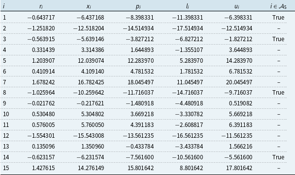
Note: Constructed example scenario data: number of scenarios $N=15$
; loss ordinal of interest
$N=15$
; loss ordinal of interest $k=5$
; risk factor scenario index i; risk factors
$k=5$
; risk factor scenario index i; risk factors $r_i$
are a pseudo-random sample from N(0,1); actual losses
$r_i$
are a pseudo-random sample from N(0,1); actual losses $x_i$
defined as a function of
$x_i$
defined as a function of $r_i$
by (54a); proxy losses
$r_i$
by (54a); proxy losses $p_i$
defined as a function of
$p_i$
defined as a function of $r_i$
by (54b); proxy lower bound
$r_i$
by (54b); proxy lower bound $l_i$
defined by (54c) satisfying
$l_i$
defined by (54c) satisfying $l_i\leq x_i$
by construction; proxy upper bound
$l_i\leq x_i$
by construction; proxy upper bound $l_i$
defined by (54d) satisfying
$l_i$
defined by (54d) satisfying $x_i\leq u_i$
by construction; the set of indices targeted for exact calculation
$x_i\leq u_i$
by construction; the set of indices targeted for exact calculation $\mathcal{A}_5$
defined in (58). The set
$\mathcal{A}_5$
defined in (58). The set $\mathcal{A}_5$
depends on the 5th largest values from each of
$\mathcal{A}_5$
depends on the 5th largest values from each of $\{l_i\}_{i=1}^{15}$
and
$\{l_i\}_{i=1}^{15}$
and $\{u_i\}_{i=1}^{15}$
, denoted
$\{u_i\}_{i=1}^{15}$
, denoted $l_{(5)}$
and
$l_{(5)}$
and $u_{(5),}$
respectively. In application, the loss scenarios
$u_{(5),}$
respectively. In application, the loss scenarios $x_i$
are expensive to compute exactly and so are unknown unless specifically targeted for exact calculation. The proxy values
$x_i$
are expensive to compute exactly and so are unknown unless specifically targeted for exact calculation. The proxy values $l_i,p_i$
and
$l_i,p_i$
and $u_i$
are assumed inexpensive to compute and risk factors
$u_i$
are assumed inexpensive to compute and risk factors $r_i$
inexpensive to generate. Through targeted exact computation, we aim to find the value
$r_i$
inexpensive to generate. Through targeted exact computation, we aim to find the value $x_{(5)}$
without exhaustive calculation of every
$x_{(5)}$
without exhaustive calculation of every $x_i$
, since exhaustive exact calculations are not feasible in practical applications. The data are displayed graphically in Panel A of Figure 1. The pseudo-random generator of Numpy (Harris et al., Reference Harris, Millman, van der Walt, Gommers, Virtanen, Cournapeau, Wieser, Taylor, Berg, Smith, Kern, Picus, Hoyer, van Kerkwijk, Brett, Haldane, del RÍo, Wiebe, Peterson, GÉrard-Marchant, Sheppard, Reddy, Weckesser, Abbasi, Gohlke and Oliphant2020) is used with fixed seed 5,000 to aid reproducibility.
$x_i$
, since exhaustive exact calculations are not feasible in practical applications. The data are displayed graphically in Panel A of Figure 1. The pseudo-random generator of Numpy (Harris et al., Reference Harris, Millman, van der Walt, Gommers, Virtanen, Cournapeau, Wieser, Taylor, Berg, Smith, Kern, Picus, Hoyer, van Kerkwijk, Brett, Haldane, del RÍo, Wiebe, Peterson, GÉrard-Marchant, Sheppard, Reddy, Weckesser, Abbasi, Gohlke and Oliphant2020) is used with fixed seed 5,000 to aid reproducibility.
We then sort the lower and upper bounds independently of each other, denoted $\{l_{(i)}\}_{i=1}^{15}$
and
$\{l_{(i)}\}_{i=1}^{15}$
and $\{u_{(i)}\}_{i=1}^{15}$
. By Lemma 2, we can bound the 5-th loss percentile without doing any exact calculations:
$\{u_{(i)}\}_{i=1}^{15}$
. By Lemma 2, we can bound the 5-th loss percentile without doing any exact calculations:
 \begin{equation}l_{(5)} \leq x_{(5)} \leq u_{(5)}.\end{equation}
This result is shown for the numerical example in Table 2 using the data from Table 1. Table 3 shows the calculation of $\mathcal{A}_5$
, the set of all scenarios whose interval of lower and upper bounds intersects with the bounds on the 5-th ordinal in (57):
$\mathcal{A}_5$
, the set of all scenarios whose interval of lower and upper bounds intersects with the bounds on the 5-th ordinal in (57):
 \begin{equation}\mathcal{A}_5 = \left\{1\leq i \leq 15\,:\, [l_i,u_i]\cap[l_{(5)},u_{(5)}]\neq\emptyset \right\} = \{1,3,8,14\}.\end{equation}
Scenarios in $\mathcal{A}_5$
are highlighted in Figure 1. Theorem 1 implies that one of the scenario indices in
$\mathcal{A}_5$
are highlighted in Figure 1. Theorem 1 implies that one of the scenario indices in $\mathcal{A}_5$
is the scenario index corresponding to the 5th largest loss
$\mathcal{A}_5$
is the scenario index corresponding to the 5th largest loss $x_{(5)}$
. However, we do not know which index without further calculation.
$x_{(5)}$
. However, we do not know which index without further calculation.
Table 2. Example numerical values used to illustrate that loss ordinals fall within proxy bound ordinals.
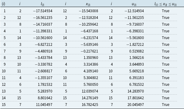
Note: Constructed example scenario data from Table 1: proxy lower loss bound $l_i$
; proxy upper loss bound
$l_i$
; proxy upper loss bound $u_i$
; actual loss
$u_i$
; actual loss $x_i$
; sorted data denoted
$x_i$
; sorted data denoted $l_{(i)},u_{(i)}$
and
$l_{(i)},u_{(i)}$
and $x_{(i)}$
; data satisfies
$x_{(i)}$
; data satisfies $l_i\leq x_i\leq u_i$
. In applications, the bounds
$l_i\leq x_i\leq u_i$
. In applications, the bounds $l_i,u_i$
are inexpensive to calculate and
$l_i,u_i$
are inexpensive to calculate and $x_i$
is expensive,
$x_i$
is expensive, $x_i$
is unknown unless a targeted exact computation is performed. The table demonstrates Lemma 1, namely that
$x_i$
is unknown unless a targeted exact computation is performed. The table demonstrates Lemma 1, namely that $l_{(i)}\leq x_{(i)}\leq u_{(i)}$
. The data are displayed graphically in Panel B of Figure 1.
$l_{(i)}\leq x_{(i)}\leq u_{(i)}$
. The data are displayed graphically in Panel B of Figure 1.
Table 3. Example numerical values used to illustrate how upper and lower bounds are updated after targeted exact computations.
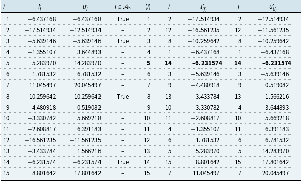
Note: Constructed example scenario data from Table 1: proxy lower loss bound $l^{\prime}_i$
; proxy upper loss bound
$l^{\prime}_i$
; proxy upper loss bound $u^{\prime}_i$
. The data are displayed graphically in Panel C and D of Figure 1. The 5th loss value (bold) is shown to have equal upper and lower bounds, indicating that proxy errors have been eliminated from this loss ordinal.
$u^{\prime}_i$
. The data are displayed graphically in Panel C and D of Figure 1. The 5th loss value (bold) is shown to have equal upper and lower bounds, indicating that proxy errors have been eliminated from this loss ordinal.
We calculate scenarios 1,3,8 and 14 exactly and update the lower and upper proxy bounds with the exact values, denoted $\{l^{\prime}_i\}_{i=1}^{15},\{u^{\prime}_i\}_{i=1}^{15}$
. We then sort the new lower and upper bounds to give
$\{l^{\prime}_i\}_{i=1}^{15},\{u^{\prime}_i\}_{i=1}^{15}$
. We then sort the new lower and upper bounds to give $\{l^{\prime}_{(i)}\}_{i=1}^{15},\{u^{\prime}_{(i)}\}_{i=1}^{15}$
. Then the 5th entry of either list gives the 5th exact loss. Therefore:
$\{l^{\prime}_{(i)}\}_{i=1}^{15},\{u^{\prime}_{(i)}\}_{i=1}^{15}$
. Then the 5th entry of either list gives the 5th exact loss. Therefore:
 \begin{equation}\hat{\xi}_{0.3} = l^{\prime}_{(5)}=u^{\prime}_{(5)}= -6.231574.\end{equation}
and we have recovered the estimate of the loss percentile without proxy error. In this example, we used four exact computations from 15 scenarios.
4. Prototypical Example
Here we show through a numerical study that it may be feasible for certain firms to remove proxy errors from their capital estimates. Even when computational budgets are limited, improvements to error bounds can be made through targeted exact computations. As a foundation, we propose an analytical distribution as a prototypical loss distribution of internal model firms, shown in Figure 4, and approximate the 0.5th percentile of the distribution. Its analytical form allows numerical investigation of computational feasibility in a representative real-life setting. The distribution is chosen to exhibit fat-tails and skew.
4.1 Computational assumptions
The capital requirement is assumed to be of the form $-x_{(k)}$
making the evaluation of
$-x_{(k)}$
making the evaluation of $x_{(k)}$
the primary objective of the study. By Theorem 1, it is sufficient to perform
$x_{(k)}$
the primary objective of the study. By Theorem 1, it is sufficient to perform $|\mathcal{A}_k|$
targeted exact computations to find the kth loss ordinal
$|\mathcal{A}_k|$
targeted exact computations to find the kth loss ordinal $x_{(k)}$
exactly. The secondary objective is to find an approximation to the bootstrap estimate of standard error of
$x_{(k)}$
exactly. The secondary objective is to find an approximation to the bootstrap estimate of standard error of $x_{(k)}$
– the expression
$x_{(k)}$
– the expression $\hat{\sigma}_{k,\varepsilon}^{*}$
is posed as a candidate for this. As discussed in section 2.8, it is sufficient to perform
$\hat{\sigma}_{k,\varepsilon}^{*}$
is posed as a candidate for this. As discussed in section 2.8, it is sufficient to perform $|\mathcal{B}_{k,\varepsilon}|$
targeted exact computations to compute the value
$|\mathcal{B}_{k,\varepsilon}|$
targeted exact computations to compute the value $\hat{\sigma}_{k,\varepsilon}^{*}$
.
$\hat{\sigma}_{k,\varepsilon}^{*}$
.
In what follows, we study the computational feasibility of eliminating proxy errors over a range of N and over a range of proxy error bounds $\Delta$
. In section 2.6, it is established that a plausible value for the number of proxy loss scenarios N is given by
$\Delta$
. In section 2.6, it is established that a plausible value for the number of proxy loss scenarios N is given by $N=1,000,000$
, and a plausible number of feasible exact loss calculations n is given by
$N=1,000,000$
, and a plausible number of feasible exact loss calculations n is given by $n=1,000$
. Therefore, for demonstration purposes, it is assumed that it is feasible to perform targeted exact computations of scenarios in the sets
$n=1,000$
. Therefore, for demonstration purposes, it is assumed that it is feasible to perform targeted exact computations of scenarios in the sets $\mathcal{A}_k$
or
$\mathcal{A}_k$
or $\mathcal{B}_{k,\varepsilon}$
whenever
$\mathcal{B}_{k,\varepsilon}$
whenever $\left|\mathcal{A}_k\right|\leq1,000$
or
$\left|\mathcal{A}_k\right|\leq1,000$
or $\left|\mathcal{B}_{k,\varepsilon}\right|\leq1,000$
, respectively.
$\left|\mathcal{B}_{k,\varepsilon}\right|\leq1,000$
, respectively.
4.2 Conclusions of numerical experiment
Figures 2 and 3 show example calculations based on the model described in section 4.3. We conclude that, in the prototypical setting:
-
It may be possible to eliminate proxy errors from capital estimates for large N if proxy error bounds are sufficiently small.
-
In this example, proxy errors can be eliminated from the capital estimate when
$N=1,000,000$
if the additive error bound is approximately £ 60m. -
The number of calculations required to approximate the bootstrap estimate of the standard error of the basic L-estimator to within
$0.1\%$
is small relative to N. -
For a fixed number of targeted exact computations, there is a choice of N which minimises error bounds (proxy plus statistical) around the true loss.
-
When the number of targeted exact computations n is computationally limited, increasing the Monte Carlo sample size N may not improve total error bounds due to the reintroduction of proxy errors.


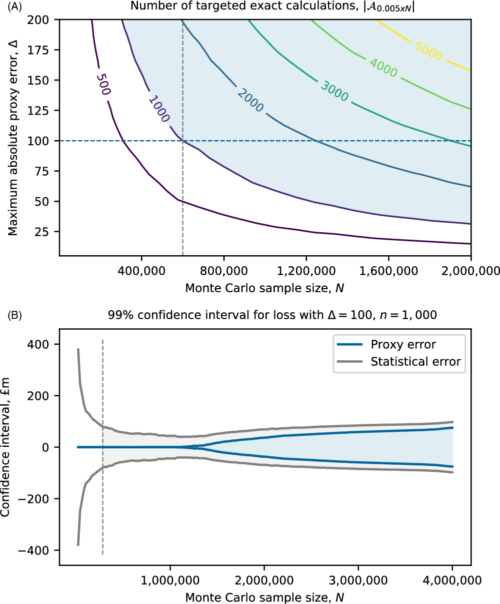
Figure 2 The method of targeted exact computation is applied to a prototypical loss distribution. Panel A: Number of exact calculations sufficient to remove proxy errors from 0.5th percentile basic L-estimator statistics, given by $\left|\mathcal{A}_{0.005\times N}\right|$
, with N proxy scenarios and proxy error bound
$\left|\mathcal{A}_{0.005\times N}\right|$
, with N proxy scenarios and proxy error bound $\Delta$
. The contours indicate feasible combinations of
$\Delta$
. The contours indicate feasible combinations of $\Delta$
and N for a given number of targeted exact computations n. The region of infeasible combinations for
$\Delta$
and N for a given number of targeted exact computations n. The region of infeasible combinations for $n>1,000$
is shaded. Panel B: Confidence interval due to statistical and proxy errors for the true 0.5th percentile loss, plotted for varying N for fixed
$n>1,000$
is shaded. Panel B: Confidence interval due to statistical and proxy errors for the true 0.5th percentile loss, plotted for varying N for fixed $\Delta=100$
and
$\Delta=100$
and $n=1,000$
. Dashed line shows maximum N at which proxy errors are removed after 1,000 targeted exact computations. In both panels, loss is a normal inverse Gaussian (NIG) random variable with parameters
$n=1,000$
. Dashed line shows maximum N at which proxy errors are removed after 1,000 targeted exact computations. In both panels, loss is a normal inverse Gaussian (NIG) random variable with parameters $a=0.6/750$
,
$a=0.6/750$
, $b=-0.2/750$
,
$b=-0.2/750$
, $\delta=750$
, and
$\delta=750$
, and $\mu=200$
.
$\mu=200$
.
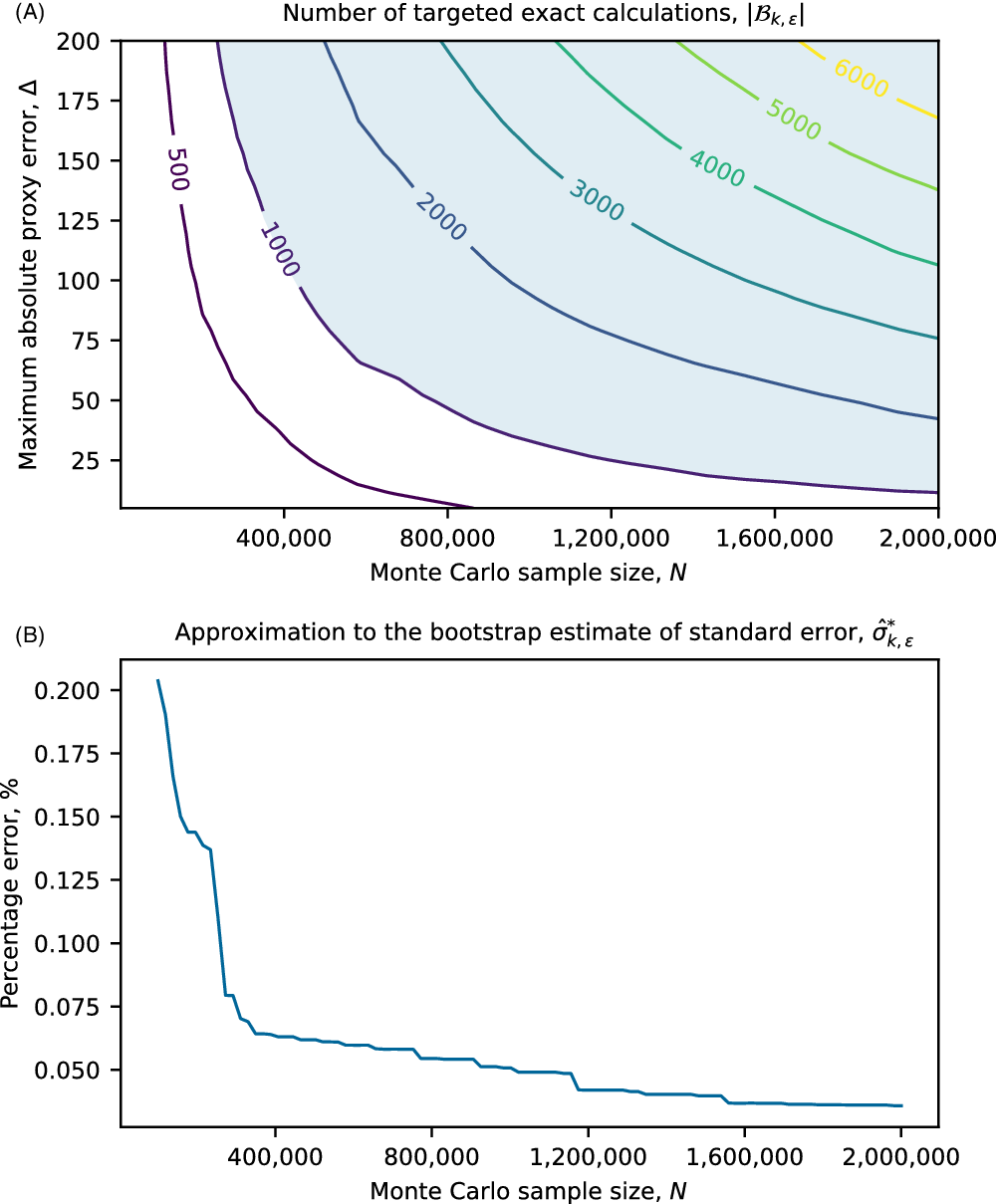
Figure 3 Panel A: Sufficient number of exact calculations, given by $\left|\mathcal{B}_{k,\varepsilon}\right|$
, to eliminate proxy errors from the bootstrap approximation of standard error, when the loss is a normal inverse Gaussian (NIG) random variable with parameters
$\left|\mathcal{B}_{k,\varepsilon}\right|$
, to eliminate proxy errors from the bootstrap approximation of standard error, when the loss is a normal inverse Gaussian (NIG) random variable with parameters $a=0.6/750$
,
$a=0.6/750$
, $b=-0.2/750$
,
$b=-0.2/750$
, $\delta=750$
, and
$\delta=750$
, and $\mu=200$
, and the 0.5th percentile is calculated using the basic L-estimator with N scenarios and proxy error bound
$\mu=200$
, and the 0.5th percentile is calculated using the basic L-estimator with N scenarios and proxy error bound $\Delta$
. For a given N we choose
$\Delta$
. For a given N we choose $\varepsilon=\varepsilon(N)$
such that
$\varepsilon=\varepsilon(N)$
such that $\sum_{j:w_j(k)>\varepsilon(N)}w_j(k)\geq0.999$
. The contours indicate feasible combinations of
$\sum_{j:w_j(k)>\varepsilon(N)}w_j(k)\geq0.999$
. The contours indicate feasible combinations of $\Delta$
and N for a given number of targeted exact computations n. The region of infeasible combinations for
$\Delta$
and N for a given number of targeted exact computations n. The region of infeasible combinations for $n>1,000$
is shaded. Panel B: Percentage error of the approximation of the bootstrap estimate of standard error, (53), relative to the actual bootstrap estimate (21) given by
$n>1,000$
is shaded. Panel B: Percentage error of the approximation of the bootstrap estimate of standard error, (53), relative to the actual bootstrap estimate (21) given by $(\sigma^*_k-\hat{\sigma}_{k,\varepsilon}^*)(\sigma^*_k)^{-1}$
. Parameter
$(\sigma^*_k-\hat{\sigma}_{k,\varepsilon}^*)(\sigma^*_k)^{-1}$
. Parameter $\varepsilon=\varepsilon(N)$
in (53) is chosen as in Panel A.
$\varepsilon=\varepsilon(N)$
in (53) is chosen as in Panel A.
In Figure 2 Panel A and in Figure 3 Panel A, the boundary of feasible and infeasible combinations of N and $\Delta$
are shown, when the feasible number of exact computations n satisfies
$\Delta$
are shown, when the feasible number of exact computations n satisfies $n\leq1,000$
. In both cases, the number of targeted scenarios increases with N and
$n\leq1,000$
. In both cases, the number of targeted scenarios increases with N and $\Delta$
. Smaller error bounds achieve both the elimination of proxy errors from capital estimates, and the possibility of reducing statistical error by increasing the sample size of proxy loss scenarios.
$\Delta$
. Smaller error bounds achieve both the elimination of proxy errors from capital estimates, and the possibility of reducing statistical error by increasing the sample size of proxy loss scenarios.
Figure 2 Panel B shows confidence intervals around the true loss from proxy and statistical errors for a fixed proxy error $\Delta=100$
and fixed number of targeted exact computations
$\Delta=100$
and fixed number of targeted exact computations $n=1,000$
. The dashed vertical line shows that proxy errors are introduced when
$n=1,000$
. The dashed vertical line shows that proxy errors are introduced when $N>600,000$
. As N increases, the proxy error initially grows slower than the statistical error reduces, and so the confidence interval becomes tighter. Past an optimal point of
$N>600,000$
. As N increases, the proxy error initially grows slower than the statistical error reduces, and so the confidence interval becomes tighter. Past an optimal point of $N\approx1,250,000$
, the proxy error grows more quickly and the confidence interval increases. This shows that when the number of possible targeted exact computations is limited (computationally), it may be sub-optimal to increase the number of Monte Carlo runs N past a certain value. On the other hand, for a fixed N, the full number of targeted exact computations
$N\approx1,250,000$
, the proxy error grows more quickly and the confidence interval increases. This shows that when the number of possible targeted exact computations is limited (computationally), it may be sub-optimal to increase the number of Monte Carlo runs N past a certain value. On the other hand, for a fixed N, the full number of targeted exact computations $\left|\mathcal{A}_{0.005\times N}\right|$
may not be required to achieve near-optimal confidence bounds.
$\left|\mathcal{A}_{0.005\times N}\right|$
may not be required to achieve near-optimal confidence bounds.
Figure 3 Panel B plots the percentage error of using $\hat{\sigma}_{k,\varepsilon(N)}^{*}$
, from (53), to approximate the bootstrap estimate of the standard error,
$\hat{\sigma}_{k,\varepsilon(N)}^{*}$
, from (53), to approximate the bootstrap estimate of the standard error, $\sigma_{k,}^{*}$
, given in (21), for varying N. The percentage error is below
$\sigma_{k,}^{*}$
, given in (21), for varying N. The percentage error is below $0.1\%$
with
$0.1\%$
with $N=300,000$
simulations. By comparison with Figure 2 Panel A and Figure 3 Panel A, in this example it is computationally feasible to eliminate proxy errors from capital estimates and approximate the bootstrap estimate of the standard error to within
$N=300,000$
simulations. By comparison with Figure 2 Panel A and Figure 3 Panel A, in this example it is computationally feasible to eliminate proxy errors from capital estimates and approximate the bootstrap estimate of the standard error to within $0.065\%$
with a fixed proxy error
$0.065\%$
with a fixed proxy error $\Delta=100$
and fixed maximum number of targeted exact computations
$\Delta=100$
and fixed maximum number of targeted exact computations $n=1,000$
.
$n=1,000$
.
4.3 Distributional assumptions
Define the prototypical loss random variable X as being a normal inverse Gaussian (NIG) random variable, introduced in Barndorff-Nielsen (Reference Barndorff-Nielsen1997), having a density function given by
 \begin{equation}f(t)=\frac{a}{\pi} \mathrm{exp}\left(\delta\sqrt{a^2-b^2}+b(x-\mu)\right)\frac{K_1\left(a\delta\sqrt{1+\frac{(x-\mu)^2}{\delta^2}}\right)}{ \sqrt{1+\frac{(x-\mu)^2}{\delta^2}}}\end{equation}
for $a,b, \delta, \mu,t\in\mathbb{R}$
, with
$a,b, \delta, \mu,t\in\mathbb{R}$
, with $0\leq|b|<a$
, and
$0\leq|b|<a$
, and $\delta>0$
, where
$\delta>0$
, where $K_1(\cdot)$
is a modified Bessel function defined by
$K_1(\cdot)$
is a modified Bessel function defined by
 \begin{equation}K_1(z) = z \int_1^\infty e^{-zt}\sqrt{t^2-1}\,\mathrm{d}t,\quad z>0.\end{equation}
We choose $a=0.6/750$
,
$a=0.6/750$
, $b=-0.2/750$
,
$b=-0.2/750$
, $\delta=750$
, and
$\delta=750$
, and $\mu=200$
, so that the 0.5th percentile loss is
$\mu=200$
, so that the 0.5th percentile loss is $\xi_{0.005}=-4465.22$
, see Figure 4 for a plot of the distribution.
$\xi_{0.005}=-4465.22$
, see Figure 4 for a plot of the distribution.

Figure 4 Prototypical loss distribution chosen to exhibit large tails and skew taking the form of a normal inverse Gaussian (NIG) distribution. The density and distribution functions are shown in Panels A and B, corresponding to NIG parameters: $a=0.6/750$
,
$a=0.6/750$
, $b=-0.2/750$
,
$b=-0.2/750$
, $\delta=750$
, and
$\delta=750$
, and $\mu=200$
.
$\mu=200$
.
In order to have lower and upper bounds that satisfy Assumption 1, suppose for any given risk factor scenario r,
 \begin{equation}l(r) = x(r) - \Delta, \quad u(r) = x(r) + \Delta,\end{equation}
for some $\Delta>0$
which we choose to vary as part of the numerical investigation. Note, by construction,
$\Delta>0$
which we choose to vary as part of the numerical investigation. Note, by construction, $l(r) \leq x(r) \leq u(r)$
for all r.
$l(r) \leq x(r) \leq u(r)$
for all r.
For a given N, we generate a sample $\{x_i\}_{i=1}^N$
using the pseudo-random NIG generator of Scipy, from which we also calculate
$\{x_i\}_{i=1}^N$
using the pseudo-random NIG generator of Scipy, from which we also calculate $\{l_i\}_{i=1}^N$
,
$\{l_i\}_{i=1}^N$
, $\{u_i\}_{i=1}^N$
,
$\{u_i\}_{i=1}^N$
, $\{l_{(i)}\}_{i=1}^N$
, and
$\{l_{(i)}\}_{i=1}^N$
, and $\{u_{(i)}\}_{i=1}^N$
. The sufficient number of calculations required in Theorem 1,
$\{u_{(i)}\}_{i=1}^N$
. The sufficient number of calculations required in Theorem 1, $\left|\mathcal{A}_{0.005\times N}\right|$
, is then found for different values of
$\left|\mathcal{A}_{0.005\times N}\right|$
, is then found for different values of $\Delta$
.
$\Delta$
.
5. Conclusions
As part of an insurer’s permission to use an internal model, detailed methodology and validation information is disclosed confidentially to the regulator. Where approximations are used, appropriate prudence must be demonstrated. The applicability of our approach to a particular firm’s internal model will depend on many factors, including whether proxy error bounds exist and have been validated, and whether pricing and actuarial systems have available the computing capacity required to perform the exact calculations within times required for business processes.
In this paper, we have focused on simulation-based capital models that utilise proxy functions. Within this setting, if a firm can find proxy error bounds (Assumption 1) and has the computing capacity to run a number of exact calculations (Assumption 2), we have shown how proxy errors can be completely removed from capital estimates, and how an approximation to the bootstrap estimate of standard error may be calculated devoid of proxy errors.
An important limitation of our approach is that it does not remove the requirement to validate proxy models. The approach shifts the validation activity onto posing and validating proxy error bounds. Also, whilst the approach is somewhat forgiving to badly fitting proxies, the number of required targeted exact computations may still be infeasibly high if poorly fitting proxies are used or if error bounds are too large.
Even if the approach is not used as part of the actual derivation of capital, it may have applications in communicating capital uncertainty, or as a validation tool to further investigate capital accuracy with findings fed back in to improving the design of proxies.
In the numerical experiment, we made the potentially surprising observation that, for a fixed computational budget for targeted exact computations, increasing the Monte Carlo sample size may not be an improvement, since doing so may increase the total error bound due to the reintroduction of proxy errors.
For future research, it is interesting to understand different approaches to posing and validating proxy error bounds, including the application of formal methods of error analysis.
Acknowledgments
This work was funded by Rothesay Life Plc where DJC and SMK are full time employees. Opinions expressed here are those of the authors and do not necessarily represent those of Rothesay. We would like to thank Shayanthan Pathmanathan for introducing us to this topic. We are also grateful to Simon Johnson and Oliver Dixon for thoughtful comments on earlier drafts and to Baptiste Grassion for his support to initiate the paper.


 Open access