


Impact Statement
The use of automated data sources in analysing transit journey time performance has gained widespread attention in the academic literature, however, the focus has been limited to the analysis of operational characteristics. Along with operational factors, passenger-specific characteristics can also influence journey times, although to date, analysis has been restricted to the evaluation of group-level demographic characteristics as this information is typically sourced via small-scale manual surveys. In this paper, we use large-scale disaggregate automated data from the London Underground metro system to track individual passengers via pseudonymised card identifiers. We apply flexible data-driven analysis methods to offer new insights regarding the degree to which individual-specific behaviours influence journey times alongside network characteristics. We find that passenger-specific characteristics have a nontrivial impact on journey times in the out-of-vehicle phases of a trip. Passenger effects represent 6% and 19% of variance in access and egress times, respectively, and this could in part be attributed to way-finding complexity within stations. For future applications, the analysis method can be used by operators to assess the relative complexity of station layouts and passenger flow control operations, as well as inform the need for potential interventions to improve passenger journey times.
1. Introduction
In this paper, we seek to quantify passenger journey time variance for trips on the London Underground metro system via a flexible data-driven analysis to identify areas for improvement in the engineering and operation of urban rail systems. Journey time variance can have a significant impact on passenger perceptions of travel. Noland and Small (Reference Noland and Small1995), Bates et al. (Reference Bates, Polak, Jones and Cook2001), and Noland and Polak (Reference Noland and Polak2002) were among the first to suggest that passenger perceptions of unreliable service arising from inconsistent journey times on a route could result in a higher generalised cost of travel. More recent studies suggest that some public transit users value consistency in journey times above reductions in mean journey times on a route (Li et al., Reference Li, Hensher and Rose2010; Kouwenhoven et al., Reference Kouwenhoven, de Jong, Koster, van den Berg, Verhoef, Bates and Warffemius2014), and empirical research on elasticities of passenger demand further indicate that improvements in journey time variance are associated with higher levels of ridership for rail transit (Preston et al., Reference Preston, Wall, Batley, Ibanez and Shires2009; van Loon et al., Reference van Loon, Rietveld and Brons2011). Better quantification of journey time variance and the factors that influence it can lead to the development of targeted interventions to improve perceptions of travel, and can ultimately lead to higher levels of ridership.
Existing research on the drivers of journey time variance for transit systems can be segmented into two distinct areas. The first research area is more network-oriented and focuses on quantifying the impact of physical and operational network characteristics on journey time performance (El-Geneidy et al., Reference El-Geneidy, Horning and Krizek2011; Sun et al., Reference Sun, Lee, Erath and Huang2012; Yetiskul and Senbil, Reference Yetiskul and Senbil2012; Ma et al., Reference Ma, Ferreira, Mesbah and Hojati2015). In this research area, there has been widespread adoption of automated data sources, including automated fare collection (AFC) data on passenger trips and automated vehicle location (AVL) data on train movements. The second area of research relates to the analysis of passenger travel behaviour and focuses on quantifying the impact of group-level sociodemographic characteristics on journey times for application in demand and choice modelling (Krygsman et al., Reference Krygsman, Dijst and Arentze2004; Crane and Takahashi, Reference Crane and Takahashi2009; McQuaid and Chen, Reference McQuaid and Chen2012; Mao et al., Reference Mao, Ettema and Dijst2018). The majority of research in this area relies on small-scale manual surveys of samples of passengers, and as a consequence of the limited scale, the influence of passenger characteristics is typically evaluated at a demographic group level rather than at the individual passenger level.
In our analysis, large-scale AFC data from the Oyster card payment system enable the identification and tracking of trips made by individual passengers via pseudonymised card numbers. Through the use of these data, we are able to quantify individual rather than group-specific effects on journey times. This more granular level of analysis can offer new insights into the influence of individual-specific characteristics on journey times, and this is a key contribution of the paper. Furthermore, the combination of the AFC trip data with AVL train movement data enables operational network characteristics as well as individual passenger-specific characteristics to be quantified. Through the use of this large-scale combined data set, we are therefore able to capture both network and passenger-specific characteristics within a unified framework to provide a more complete and precise characterisation of the drivers of journey time variance compared to previous studies.
The analysis is split into two parts: (i) passenger journey times are decomposed into components to distinguish between in- and out-of-vehicle phases of a passenger journey via a probabilistic assignment algorithm to allocate individual passenger trips to unique train itineraries, and (ii) semiparametric regression is used to quantify the effects of passenger-level heterogeneity and network-related factors within each component of journey time, as well as total journey times. Semiparametric regression is a data-driven analysis technique whereby the relationships between the independent and dependent variables are generated via flexible splines fitted to the data points, thus resulting in a greater degree of fidelity to the data compared to conventional linear regression methods. In the literature on the generalised cost of travel for rail modes, it is well established that the out-of-vehicle phases of a journey are considered to be more onerous for passengers compared to base uncongested in-vehicle travel conditions. Walking and wait time components are typically valued at least twice the value of uncrowded in-vehicle times (Wardman, Reference Wardman2004; Wardman et al., Reference Wardman, Chintakayala and de Jong2016). In this analysis, we therefore consider the in-vehicle and out-of-vehicle components of journey time separately.
The results from the analysis can provide valuable insights for transit operators regarding the management of journey time variance. For total journey times, we find that train speeds and headways represent the majority of variance while passenger heterogeneity represents a minimal proportion, and that static route-specific characteristics are more influential than passenger-specific effects. However, within the typically twice as onerous out-of-vehicle components of access and egress times, passenger characteristics are found to be more influential. Passenger-specific effects are similarly or more influential than static network effects, and on average, passenger-level heterogeneity represents 19% of variance in egress times and 6% of variance in access times. Although quantification of the generalised cost of travel is not within the scope of this analysis, the results indicate that the impact of passenger heterogeneity in the access and egress models would be nontrivial in terms of passenger perceptions of travel.
The estimates of passenger heterogeneity obtained in this analysis have potential applications related to improving the understanding of passenger movements within stations. Across all stations in the analysis, a greater degree of passenger heterogeneity is observed in the egress phase compared to the access phase. A lower degree of heterogeneity in the access models could be a result of the constraint imposed on passenger walking speeds and platform positioning to board the train when it arrives, while no such constraints are present in the egress phase. The result could also reflect a greater degree of way-finding complexity as a result of complex station layouts with poor route information, or less effective pedestrian flow control measures (for example, less availability of dynamically controlled escalators in the exiting direction). Further modelling of disaggregate station elements could disentangle such effects. Furthermore, the analysis could be undertaken at an individual station or route level, and differences in passenger-level heterogeneity could be used to identify differences in way-finding complexity between stations. The second stage modelling of disaggregate station characteristics could then guide operators in identifying station elements that require potential improvements. The estimates of passenger heterogeneity obtained in this analysis could also be used as inputs to improve assumptions of passenger walking characteristics in pedestrian modelling applications used in the assessment of pedestrian dynamics and flows in transit stations.
The remainder of the paper is organised as follows: a literature review is presented in Section 2, and the study area and the properties of the data set are defined in Section 3. The framework for the semiparametric regression models is given in Section 4. The analysis and discussion of the results are presented in Section 5, and conclusions are summarised in Section 6.
2. Literature review
Prior to the introduction of automated data collection systems, the observation of passenger travel patterns relied on data obtained from manual stated preference surveys (SP) and passenger counts. The increasing prevalence of AFC systems has enabled access to greater volumes of passenger trip data and more detailed information on passenger travel patterns in a revealed preference (RP) format. AFC systems capture information on trip transactions as well as card properties, which can represent passenger-specific information, however, the recorded information can vary in level of detail. Trip information can include entry and exit dates, times, and locations. In a number of cases, boarding or alighting locations are not recorded, and so there are a number of approaches in the literature to infer missing timestamps and location information, including the work by Trepanier et al. (Reference Trepanier, Chapleau and Tranchant2007) and Munizaga and Palma (Reference Munizaga and Palma2012). Card-specific information typically includes unique card identification numbers and the card payment category, which captures price differentiation based on user segmentation. In the registration process for AFC cards, additional information may also be recorded including home address, age, gender, occupation, and bank account details.
Research seeking to quantify the impact of passenger characteristics on transit journey times is largely based on analysing group-level characteristics where passengers are aggregated into user groups to represent different population demographics. Research targeted at the level of individual passengers is limited, with only one known study undertaken on analysing the consistency of departure times of individual commuters using SP data in Germany by Kitamura et al. (Reference Kitamura, Yamamoto, Susilo and Axhausen2006). To that end, the following literature review not only covers work on transit journey times, but also includes a review of work in the wider transport literature which focuses on the analysis of passengers at an individual level using RP data from AFC systems. Research areas include the analysis of individual travel patterns in transit networks, and the development of individual-specific route choice models.
2.1. Travel patterns
The majority of research that makes use of passenger-specific information recorded by AFC systems focuses on recovering descriptive information on the travel patterns of individuals. Utsunomiya et al. (Reference Utsunomiya, Attanucci and Wilson2006), Morency et al. (Reference Morency, Trepanier and Agard2007), Trepanier et al. (Reference Trepanier, Habib and Morency2012), and Goulet-Langlois et al. (Reference Goulet-Langlois, Koutsopoulos and Zhao2016) use AFC data with complete tap-in and tap-out information recorded. Utsunomiya et al. (Reference Utsunomiya, Attanucci and Wilson2006) mine individual-level travel behaviour using AFC data from rail, bus, and paratransit in Chicago. Access distances for the first transit trip of the day are analysed, along with the frequency of trips and consistency of routes taken. Another study on individual travel patterns is undertaken by Morency et al. (Reference Morency, Trepanier and Agard2007) using smart card data from the bus network in Gatineau, Canada. Data segmentation and a k-means clustering algorithm are applied to determine spatial and temporal patterns of bus boarding by passenger card type. The analysis for the Gatineau bus network is extended by Trepanier et al. (Reference Trepanier, Habib and Morency2012), where a hazard model is applied to determine the degree of loyalty of individual passengers using the service and the underlying socioeconomic factors affecting loyalty. Goulet-Langlois et al. (Reference Goulet-Langlois, Koutsopoulos and Zhao2016) use data from bus and rail modes in London, UK, and apply principal component analysis and the k-means
 $ ++ $
clustering algorithm to segment passengers into 11 different clusters based on their travel activity patterns. A further analysis is undertaken using odds-ratios to understand the relationship between travel patterns and sociodemographic passenger information collected through household travel surveys.
$ ++ $
clustering algorithm to segment passengers into 11 different clusters based on their travel activity patterns. A further analysis is undertaken using odds-ratios to understand the relationship between travel patterns and sociodemographic passenger information collected through household travel surveys.
In the studies undertaken by Ma et al. (Reference Ma, Wu, Wang, Chen and Liu2013) and Kieu et al. (Reference Kieu, Bhaskar and Chung2015), the AFC data have missing timestamp and location information, so an additional step to infer the missing information is first performed. Ma et al. (Reference Ma, Wu, Wang, Chen and Liu2013) analyse the spatial and temporal travel patterns of individuals for the bus and metro systems in Beijing, China. The data do not record boarding and alighting locations and tap-out timestamps and so a decision tree algorithm is first applied to infer the locations and further clustering algorithms are applied, including the density-based spatial clustering algorithm (DBSCAN), to infer the regular and irregular travel routes and times for individuals. A similar analysis is performed by Kieu et al. (Reference Kieu, Bhaskar and Chung2015) on bus, rail, and ferry data from Brisbane, Australia. Complete origin–destination (OD) trip chains are first constructed for passengers who use more than one mode for a given trip, and then the DBSCAN algorithm is applied to infer regular travel routes and regular travel times of individual passengers.
2.2. Route choice modelling
The broader field of travel behaviour research focuses on analysing the effects of sociodemographic characteristics on travel behaviour, and the majority of these studies use SP survey data and population census data. Within this field, travel utility theory methods are applied to infer travel preferences and decision making at a user-group level; reviews of the more recent advances in travel behaviour analysis at a household level can be found in Bhat and Pendyala (Reference Bhat and Pendyala2005) and Timmermans and Zhang (Reference Timmermans and Zhang2009). Focusing on rail networks in particular, travel behaviour models are used to quantify the route choice of passengers between each origin and destination node of a network, and this has conventionally been undertaken through SP surveys of samples of passengers, e.g., Guo and Wilson (Reference Guo and Wilson2011) and Raveau et al. (Reference Raveau, Guo, Munoz and Wilson2017).
Recent work incorporates the more disaggregate information available from AFC sources to develop improved models of route choice based on the generation of individual utility functions rather than the traditional approach, which estimates utility functions for the average user based on aggregation of individual preferences from a sample of passengers. Arentze (Reference Arentze2013), Nuzzolo et al. (Reference Nuzzolo, Crisalli, Comi and Rosati2015), and Nuzzolo and Comi (Reference Nuzzolo and Comi2016) estimate route choice preferences at an individual level for input into transit trip planner tools. Nuzzolo et al. (Reference Nuzzolo, Crisalli, Comi and Rosati2015) and Nuzzolo and Comi (Reference Nuzzolo and Comi2016) develop route choice utility functions at an individual level for public transit networks in Rome, beginning with a stated preference survey filled out by users to establish their initial preferences, and then preferences are iteratively updated with revealed preference data of recorded trips that the individual has taken. Arentze (Reference Arentze2013) follows a similar approach, however in this case, initial user preferences are designated as the average of aggregated travel preferences of users from SP survey data from a sample of passengers. Aside from these three studies on transit modes, the remaining majority of work on analysing route choice at an individual level focuses more on private road transport with revealed preference data generated from vehicle-mounted GPS trackers, as presented in Li et al. (Reference Li, Miwa, Morikawa and Liu2016), Lima et al. (Reference Lima, Stanojevic, Papagiannaki, Rodriguez and Gonzalez2016), and Amirgholy et al. (Reference Amirgholy, Golshani, Schneider, Gonzales and Gao2017).
2.3. Journey time modelling
Compared to the descriptive work on tracking individual travel patterns, and studies on inferring route choice at an individual level, assessing the impact of individual-level heterogeneity on journey times has received relatively little attention in the literature. Kitamura et al. (Reference Kitamura, Yamamoto, Susilo and Axhausen2006) use stated preference data gathered from 6-week travel diaries of inhabitants in Karlsruhe and Halle in Germany to track the consistency of departure times by individuals for the first morning trip of the day. Linear regression and stochastic frontier models are applied to determine the degree of intra-individual and inter-individual heterogeneity in departure times, including additional explanatory variables to capture sociodemographic characteristics such as gender, income, residential zone, household size, marriage status, and total commuting time.
The remaining majority of the literature involves aggregation of individual passengers into categories and therefore, the interpretation of results can only be applied at a group rather than individual level. For example, in transport sociology literature, a vast stream of research is dedicated to analysing gender-based differences in journey times (Crane, Reference Crane2007; Crane and Takahashi, Reference Crane and Takahashi2009; McQuaid and Chen, Reference McQuaid and Chen2012). Another branch of research involves developing regression models of journey time for travel demand and behaviour applications. The regression models typically include sociodemographic characteristics such as age, occupation, income, ethnicity, household characteristics, and residential zone, among others (Krygsman et al., Reference Krygsman, Dijst and Arentze2004; Fan and Machemehl, Reference Fan and Machemehl2009; Mao et al., Reference Mao, Ettema and Dijst2018).
Thus from our review of the literature, we find that analyses of travel characteristics at an individual level have focused more on the descriptive characterisation of travel patterns and inference of route choice behaviour. Work on quantifying the underlying drivers of transit journey times focuses more on analysing the impact of passenger characteristics at a group rather than individual level. The analysis presented in this paper aims to combine network and passenger-related factors in a unified modelling framework to better inform operators of the drivers of journey time variance. Rather than representing passengers at a group level, we make a new contribution to the literature by exploiting the disaggregate information recorded by the London Underground AFC Oyster card system to analyse the impact of heterogeneity at an individual passenger level along with operational and physical network characteristics.
3. Study area and data
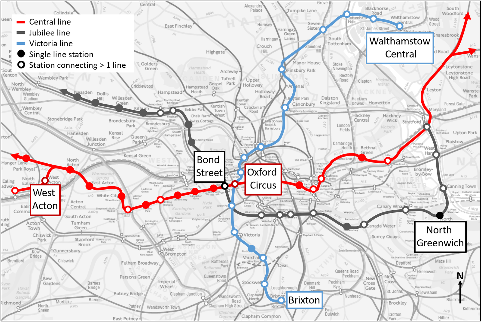
Selected sections of three lines on the London Underground are included in the analysis, and these line sections are located within the Transport for London (TfL) zones 1 and 2 in the Central London area. The line sections are chosen to exclude considerations of route choice and interchange movements. As a result, trips within the study area satisfy the following conditions: (i) trips are single line trips that originate and terminate on the same line and (ii) there are no other probable routes between the OD pair of interest under normal operating conditions. Trips in both directions are analysed over the following topological extents: the entire length of the Victoria line (16 stations), West Acton to Oxford Circus on the Central line (12 stations), and Bond Street to North Greenwich on the Jubilee line (10 stations). The analysis boundaries are illustrated in Figure A1 in Appendix A.
Weekday trips (Monday–Friday) over a 7 week period from October to December 2013 are analysed. The TfL Oyster smart card system records tap-in and tap-out timestamps and locations at the origin and destination stations for each trip. The TfL NetMIS system records train departure timestamps at each station platform in the network. Additional data on the physical and operational characteristics of the network are obtained through TfL infrastructure and operations database sources and station layout drawings.
For the analysis of individual characteristics, multiple observations of an individual passenger completing trips on the same OD route are required. Figure 1 shows the frequency distribution of the number of trips an individual passenger undertakes on the same OD pair within the analysis boundaries. As shown in the figure, the majority of trips are undertaken by passengers who travel infrequently, with over half of trips undertaken by passengers who complete fewer than three repeat trips on the same OD pair.

Figure 1. Distribution of the number of trips undertaken on the same origin–destination (OD) route per individual passenger.
In the selection of the range of trip frequencies, there is a trade-off between ensuring that there are enough observations per passenger for robust estimation of model parameters and the computational time required to successfully generate the regression models. Using the “mgcv” package in R statistical analysis software, the time taken for the semiparametric regression models to converge to a solution is in the order of
 $ O(np) $
where
$ O(np) $
where
 $ n $
is the number of observations in the data set and
$ n $
is the number of observations in the data set and
 $ p $
is the number of model parameters to be estimated (Wood et al., Reference Wood, Goude and Shaw2015). In this analysis, each individual passenger is treated as a unique parameter in the model. Therefore, including more passengers in the data set leads to longer computational times.
$ p $
is the number of model parameters to be estimated (Wood et al., Reference Wood, Goude and Shaw2015). In this analysis, each individual passenger is treated as a unique parameter in the model. Therefore, including more passengers in the data set leads to longer computational times.
Through a number of trials, we select a random sample of 8,000 passengers who complete 10 or more repeat trips on the same OD route as the data set to be used in the analysis. The selection of a minimum number of 10 trips enables enough repeat trips per passenger for regression modelling purposes, as well as being representative of a range of passengers from those who travel less frequently to those who travel on the same route everyday over the 35 day analysis period. The frequency distribution of the selected subset of trips by the time of day is illustrated in Figure 2. The figure shows that the sample represents typical weekday travel patterns where more passenger trips are undertaken during the morning and afternoon peak periods, compared to the midday inter-peak.
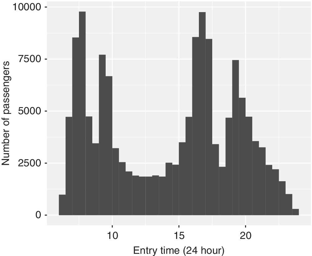
Figure 2. Distribution of sampled passenger trips by time of day.
4. Methods
The AFC data set reports total journey times from tap-in at the origin station to tap-out at the destination station, and to enable the journey times to be split into parts, passengers must first be allocated to trains. This is achieved by merging the AFC trip data with the AVL train movement data and applying a probabilistic train assignment algorithm based on the egress times associated with each feasible train itinerary. Full details of the assignment algorithm are not presented here but are available in Singh et al. (Reference Singh, Hörcher, Graham and Anderson2020).
Through assignment of all trips to unique train itineraries, the total journey times of each trip are decomposed to obtain the access, on-train, and egress time components. Semiparametric regression models are then developed with the components of journey time set as the response variables, as detailed in the following sections.
4.1. General regression model framework
Semiparametric regression enables nonlinear relationships between the independent and dependent variables to be modelled via basis functions in the form of penalised thin-plate regression splines. The basis functions are fitted with a penalty to impose a trade-off between the degree to which the spline functions match the data and the degree of smoothness. Further details of the underlying theory are given in Wood et al. (Reference Wood, Goude and Shaw2015) and Wood (Reference Wood2017). Model fitting is undertaken using penalised iteratively reweighted least squares (PIRLS), and the model parameters are estimated via restricted maximum likelihood (REML) optimisation (Wood et al., Reference Wood, Goude and Shaw2015; Wood, Reference Wood2017).
A generalised additive mixed model (GAMM) framework is used, and a log–log form produces the best performing models in terms of goodness-of-fit. Further discussion and comparisons of different model forms are presented in Section 5.2. The resulting general form of the regression models is given in Equation (1). To facilitate subsequent interpretation of the results, the exponential form of Equation (1) is given in Equation (2).
 $$ \log \left({Y}_{ijt}\right)=\alpha +\sum \limits_{k=1}^K{f}_k\left(\log \left({X}_{ijt}\right)\right)+{u}_i+{c}_j+{\gamma}_t+{\varepsilon}_{ijt} $$
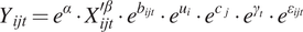 $$ {Y}_{ijt}={e}^{\alpha}\cdot {X}_{ijt}^{\hbox{'}\beta}\cdot {e}^{b_{ijt}}\cdot {e}^{u_i}\cdot {e}^{c_j}\cdot {e}^{\gamma_t}\cdot {e}^{\varepsilon_{ijt}} $$
In Equations (1) and (2),
 $ {Y}_{ijt} $
is the response calculated as
$ {Y}_{ijt} $
is the response calculated as
 $ \left(\frac{y_{ijt}^c}{y_{fj}^c}\right) $
, where
$ \left(\frac{y_{ijt}^c}{y_{fj}^c}\right) $
, where
 $ {y}_{ijt}^c $
is component
$ {y}_{ijt}^c $
is component
 $ c $
of journey time evaluated for passenger
$ c $
of journey time evaluated for passenger
 $ i $
travelling on a given OD route, via given entry and exit stations on a given line and direction. The network group effects specific to each unique OD route are collectively denoted by
$ i $
travelling on a given OD route, via given entry and exit stations on a given line and direction. The network group effects specific to each unique OD route are collectively denoted by
 $ j $
,
$ j $
,
 $ t $
denotes the day of travel, and
$ t $
denotes the day of travel, and
 $ {y}_{fj}^c $
is the free flow time on the route. The model constant is denoted by
$ {y}_{fj}^c $
is the free flow time on the route. The model constant is denoted by
 $ \alpha $
,
$ \alpha $
,
 $ {X}_{ijt} $
are the covariates modelled nonparametrically, and
$ {X}_{ijt} $
are the covariates modelled nonparametrically, and
 $ {f}_k,k=1..K $
are the smooth basis functions based on penalised thin-plate regression splines such that
$ {f}_k,k=1..K $
are the smooth basis functions based on penalised thin-plate regression splines such that
 $ {f}_k\left(\log \left({X}_{ijt}\right)\right)=\beta \log \left({X}_{ijt}^{\prime}\right)+{b}_{ijt},{b}_{ijt}\sim \mathcal{N}\left(0,{\sigma}_b^2\right) $
(Wood, Reference Wood2017). The group-specific fixed effects for the categorical factors of OD routes, stations, and line/directions are collectively represented by
$ {f}_k\left(\log \left({X}_{ijt}\right)\right)=\beta \log \left({X}_{ijt}^{\prime}\right)+{b}_{ijt},{b}_{ijt}\sim \mathcal{N}\left(0,{\sigma}_b^2\right) $
(Wood, Reference Wood2017). The group-specific fixed effects for the categorical factors of OD routes, stations, and line/directions are collectively represented by
 $ {c}_j $
,
$ {c}_j $
,
 $ {u}_i $
are the passenger-specific random effects, such that
$ {u}_i $
are the passenger-specific random effects, such that
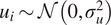 $ {u}_i\sim \mathcal{N}\left(0,{\sigma}_u^2\right) $
,
$ {u}_i\sim \mathcal{N}\left(0,{\sigma}_u^2\right) $
,
 $ {\gamma}_t $
are the fixed effects indexing the different days
$ {\gamma}_t $
are the fixed effects indexing the different days
 $ t $
of travel, and
$ t $
of travel, and
 $ {\varepsilon}_{ijt} $
is the random error term such that
$ {\varepsilon}_{ijt} $
is the random error term such that
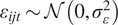 $ {\varepsilon}_{ijt}\sim \mathcal{N}\left(0,{\sigma}_{\varepsilon}^2\right) $
.
$ {\varepsilon}_{ijt}\sim \mathcal{N}\left(0,{\sigma}_{\varepsilon}^2\right) $
.
The systematic component of the regression model comprises continuous covariates which capture observed variation in the model, and categorical factors which capture unobserved variation between groups of categories modelled as fixed and random effects. The continuous covariates are modelled via nonparametric thin-plate regression splines generated from the data points; these smooth basis functions also possess a random effects structure to accommodate uncertainty in the estimation of the smoothing parameters, and this has implications for the interpretation of the model results as discussed further in Section 5.4. In terms of the group-specific effects, the main distinction between the two forms is that fixed effects allow correlation between group effects and other covariates, while random effects do not allow correlation.
Fixed effects can be interpreted as constants specific to each level within a factor. A fixed effects structure is more appropriate if the variable has been drawn from a finite population, where inferences regarding the effect of the variable are confined to the categories of the variable included in the model (Searle et al., Reference Searle, Casella and McCulloch1992). The fixed effects structure is applied for stations, OD routes, line/directions, and days.
Conversely, a random effects structure is more appropriate in cases where the variable has been drawn from a large or infinite population, and the observations used in the model are considered a random sample of the population (Searle et al., Reference Searle, Casella and McCulloch1992). Under a random effects structure, the random effects coefficients are considered to be independently and identically distributed with mean 0 and constant variance. As the individual passengers in the analysis represent a sample of a large population of passengers in London, passenger-specific effects are modelled as random effects. Validation of the fixed and random effects designations is undertaken and documented in the discussion of model results in Section 5.2.
4.2. Dependent variables
The dependent variable in Equations (1) and (2) represents the journey time of each passenger trip at a component level
 $ {y}_{ijt}^c $
normalised by the average free flow time at a component level
$ {y}_{ijt}^c $
normalised by the average free flow time at a component level
 $ {y}_{fj}^c $
. The free flow time represents the time taken to travel from the origin to the destination in uncongested conditions without delays, and it is taken here as the 10th percentile of the aggregate journey time distribution for the OD pair of interest over the 7-week analysis period. The 10th percentile value is chosen as it is not influenced by outlying journey times recorded for the fastest individuals travelling in ideal situations, for example, a passenger running through an empty station to board the train just as it arrives. The rationale behind the choice of the free-flow normalised response variable is that the explanatory variables capture variation in journey times relative to the base uncongested travel conditions on a route.
$ {y}_{fj}^c $
. The free flow time represents the time taken to travel from the origin to the destination in uncongested conditions without delays, and it is taken here as the 10th percentile of the aggregate journey time distribution for the OD pair of interest over the 7-week analysis period. The 10th percentile value is chosen as it is not influenced by outlying journey times recorded for the fastest individuals travelling in ideal situations, for example, a passenger running through an empty station to board the train just as it arrives. The rationale behind the choice of the free-flow normalised response variable is that the explanatory variables capture variation in journey times relative to the base uncongested travel conditions on a route.
Journey times are split into four components and analysed in three distinct time periods and so a total of 12 models are estimated. The components of journey time are defined as follows: (i) Access time is the time between passenger tap-in at the origin station and the departure of the assigned train at the origin station, (ii) On-train time is the time between train departure at the origin station and train departure at the destination station, (iii) Egress time is the time from train departure at the destination station to passenger tap-out at the destination station, and (iv) Total journey time is the total time from passenger tap-in at the origin station to passenger tap-out at the destination station. The time of day is arranged into three subcategories as follows: (i) AM peak—7 am to 10 am, (ii) Inter-peak—10 am to 4 pm, and (iii) PM peak—4 pm to 7 pm.
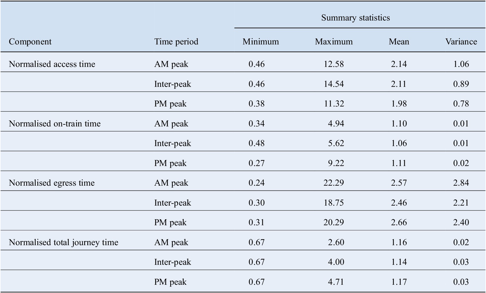
The descriptive statistics for the dependent variables corresponding to the 12 regression models are summarised in Table 1. Across all time periods, on-train times are the least variable component, followed by total journey times, while access and egress times are relatively more dispersed. Across all components, mean journey times tend to be longest during the AM peak and PM peak periods compared to the midday inter-peak. This coincides with the distribution of passenger entries by time of day as shown in Figure 2, which indicates that more trips are undertaken in the peaks compared to the inter-peak.
Table 1. Summary statistics of dependent variables.
To further contextualise the components of journey time, Figure 3 illustrates the shares of access, on-train, and egress times as a proportion of total journey times. On average, on-train times represent the greatest proportion of total journey times (64%), followed by access times (25%), and egress times (11%).

Figure 3. Proportional share of journey time components relative to total journey time.
4.3. Model covariates
4.3.1 Group-specific effects
Individual-level effects - The effects of the passenger characteristics are captured at an individual card level. The pseudonymised unique card identifiers are defined as categorical factors in the models, and are modelled as random effects. The number of individual passengers by time period is summarised in Table 2. Across all time periods, passengers make on average approximately 16 repeat trips on the same OD route over the 35-day analysis period. Analysing the properties of the data set, 84% of trips in the AM peak, 71% in the inter-peak, and 84% in the PM peak are made by adults holding Oyster cards with no additional discounts applied. The remaining trips are associated with a mix of child, student, and senior card holders.
Table 2. Number of passengers per time period.

Stations, OD routes, and line/direction effects - Rather than explicitly including different measures for different physical characteristics, each station, OD route, and line/direction are defined as a fixed effects categorical variable, which represents all physical characteristics and any other residual time-invariant properties associated with the entity.
Days - Fixed effects at the level of days are included to account for changes in travel conditions across the 35-day analysis period.
The number of levels within each fixed effects category by model is given in Table 3.
Table 3. Summary of fixed effects levels.

Abbreviation: OD, origin–destination.
4.3.2 Continuous covariates
Headway - Different service frequencies are in operation at different times of the day on different lines, and this can lead to fluctuations in journey times. The headway for each trip is therefore included in the models and is measured on a minutes scale.
Coefficient of variation (COV) of headway - The coefficient of variation of headway is included to capture the variation in train frequencies which would otherwise skew the model results, particularly at the transition periods between peak and off-peak times. The COV is calculated over the 15 min period corresponding to the time that the trip was undertaken at an OD route level.
Headway normalised by mean headway - The train headway associated with each passenger trip is normalised by the mean value of headway over the corresponding period of 15 min at an OD route level. This covariate is included to specifically capture any potential effects of train bunching. In the train movement data set, approximately 15% of all trips operate at headways shorter than the minimum scheduled headway of approximately 1.67 min, and this may indicate the occurrence of train bunching.
Train speed - Train speed is included as a covariate in the on-train time and total journey time models, and it is calculated by taking the inter-station distance of each trip and dividing by the on-train time of the trip. To maintain consistency in units with the other covariates in the models, speed is measured here in kilometers per minute.
Passenger demand indicators - A set of covariates are included to represent passenger demand levels. Indicators of passenger volumes are evaluated at three points as follows: platform loading at the origin station, line loading, and platform loading at the destination station. Since trips by Oyster card captured an estimated 70% share of all trips made on the network in 2013 (Uniman, Reference Uniman2009; Paul, Reference Paul2010), the indicators of passenger loading are calculated using the TfL Rolling Origin and Destination survey (RODs), which provides count estimates of all trips on the network. The indicator for passenger volumes
 $ {\rho}_{qpt} $
for the quantity of interest
$ {\rho}_{qpt} $
for the quantity of interest
 $ q $
(origin platform loading, line loading, destination platform loading) is defined as the number of trips
$ q $
(origin platform loading, line loading, destination platform loading) is defined as the number of trips
 $ {n}_{qpt} $
during a 15 min time period
$ {n}_{qpt} $
during a 15 min time period
 $ p $
on day
$ p $
on day
 $ t $
, normalised by the average number of trips
$ t $
, normalised by the average number of trips
 $ {\overline{n}}_{qt} $
across all 15 min periods over the day as per Equation (3).
$ {\overline{n}}_{qt} $
across all 15 min periods over the day as per Equation (3).
 $$ {\rho}_{qpt}=\frac{n_{qpt}}{{\overline{n}}_{qt}}. $$
5. Results
5.1. Data properties
Testing of correlations between covariates is performed to determine the degree of linear association via Pearson correlation testing and for the presence of nonparametric monotonic associations through Spearman correlation testing. The correlation matrices show that the highest degree of correlation occurs between the covariates representing headways and normalised headways. The Spearman correlation coefficient has a maximum value of 0.76 and the Pearson correlation coefficient has a maximum value of 0.73. The maximum values of the correlation coefficients do not indicate strong correlations between the covariates. Moreover, given the large volume of data available for model estimation, it is appropriate to initially include all covariates in the models and conduct further model refinement based on covariate significance values as required.
5.2. Model form
The results of alternate model forms are presented in Appendix B to justify the application of the following: the GAMM form with continuous covariates modelled with smooth splines and group-specific effects modelled with mixed fixed and random effects, the log-log transformation, and the random effects structure for the passenger-specific effects. The model goodness-of-fit statistics for four model forms are presented in Tables B1–B4 in Appendix B corresponding to: (i) Final model form—all continuous covariates modelled with nonparametric smooths, fixed network effects, and random passenger effects (Table B1), (ii) All continuous covariates modelled with nonparametric smooths, fixed network effects, and fixed passenger effects (Table B2), (iii) All continuous covariates modelled with nonparametric smooths, fixed network effects, random passenger effects, and with no log transformations applied to any variables (Table B3), and (iv) All continuous covariates modelled with a linear structure, and no group-specific effects (Table B4). It should be noted that as a result of previous trials of model form, the covariates capturing the network effects are modelled as fixed effects in the final model form. The passenger-specific effects are found to be significant at a level of 99.9% in the access, egress, and total journey time models; however, they are not significant in the on-train time models at a lower bound of 90% significance. This result is as expected; the network operational characteristics and physical route characteristics are the primary determinants of the variance in on-train times. Consequently, the results for the on-train time models are not further presented.
The justification for the log-log transformation can be ascertained by comparing the results for the final model form (Table B1) and the equivalent model form with no log transformations applied (Table B3). Although the models with no log transformations perform slightly better in terms of the indicators that reflect how well the models represent variation in the data (
 $ {R}_{adj.}^2 $
and
$ {R}_{adj.}^2 $
and
 $ {D}_{explained} $
), the remaining three indicators for overall model performance (AIC, BIC, REML) perform worse than the log-transformed form. As such, it can be stated that the log-transformed models provide a better overall fit to the data. From a theoretical perspective, the log-transformation applied to the response variable of journey times also corresponds to the literature on transit journey time distributional form, which states that journey times are typically distributed following a right-skewed form (Fosgereau and Fukuda, Reference Fosgereau and Fukuda2012; Taylor and Susilawati, Reference Taylor and Susilawati2012; Rahman et al., Reference Rahman, Wirasinghe and Kattan2018).
$ {D}_{explained} $
), the remaining three indicators for overall model performance (AIC, BIC, REML) perform worse than the log-transformed form. As such, it can be stated that the log-transformed models provide a better overall fit to the data. From a theoretical perspective, the log-transformation applied to the response variable of journey times also corresponds to the literature on transit journey time distributional form, which states that journey times are typically distributed following a right-skewed form (Fosgereau and Fukuda, Reference Fosgereau and Fukuda2012; Taylor and Susilawati, Reference Taylor and Susilawati2012; Rahman et al., Reference Rahman, Wirasinghe and Kattan2018).
The verification of the GAMM structure is assessed by comparing the final form, which consists of continuous covariates modelled with nonparametric smooths and mixed fixed and random group-specific effects (Table B1), with the base pooled linear model form in Table B4, where the continuous covariates are modelled with a linear form and there are no group-specific effects. The base pooled linear model form tends to perform better than the GAMM structure when considering the BIC indicator which penalises more heavily for model complexity. However, across all other goodness-of-fit criteria, the GAMM form outperforms the base linear model form. As such, we adopt the GAMM form as the final form for all models.
Comparing the random and fixed effects structures for the passenger effects, Tables B1 and B2 show that the performance of the two forms is similar. Across all models, the
 $ {R}_{adj.}^2 $
indicator reflects equal performance for the two forms. The
$ {R}_{adj.}^2 $
indicator reflects equal performance for the two forms. The
 $ {D}_{explained} $
indicates that the fixed effects form performs better, while the AIC and BIC indicate that the random effects structure performs better across all models. The REML scores are mixed, indicating that the fixed effects structure is more appropriate for the egress time models and the inter-peak access time model, and that the random effects structure is more appropriate for the remaining models. Overall, the results show that the majority of models perform better with a random effects structure. Coupled with the theoretical basis for the application of a random effects structure for the passenger effects, this form is adopted for the final models.
$ {D}_{explained} $
indicates that the fixed effects form performs better, while the AIC and BIC indicate that the random effects structure performs better across all models. The REML scores are mixed, indicating that the fixed effects structure is more appropriate for the egress time models and the inter-peak access time model, and that the random effects structure is more appropriate for the remaining models. Overall, the results show that the majority of models perform better with a random effects structure. Coupled with the theoretical basis for the application of a random effects structure for the passenger effects, this form is adopted for the final models.
5.3. Covariate significance and mean elasticities
The passenger effects are significant at a level of 99.9% in all access, egress, and total journey time models. The group-specific fixed effects for days, stations, OD routes, and line/direction are also significant in all models; however, the significance levels vary across the groups from a minimum level of significance
 $ \ge $
90% to a maximum level of significance
$ \ge $
90% to a maximum level of significance
 $ \ge $
99.9%. The passenger effects and fixed effects representing network characteristics are discussed further in Section 5.4.
$ \ge $
99.9%. The passenger effects and fixed effects representing network characteristics are discussed further in Section 5.4.
The significance and mean elasticities of the continuous covariates are given in Table 4. Overall, the models generate plausible results in terms of the relative magnitudes and directions of elasticity. For the access time models across all time periods, headways are the most influential covariate, with a positive mean elasticity representing longer platform wait times as headways increase. The covariates representing passenger demand levels are the second most influential set of covariates, while the covariates representing headway regularity have a relatively low degree of impact on access times.
Table 4. Results for continuous covariates.

Abbreviations: COV, Coefficient of variation.
Significance notation: p-values 0 ‘***’ 0.001 ‘**’ 0.01 ‘*’ 0.05 ‘.’ 0.1 ‘’ 1
Compared to the magnitude of elasticities of covariates in the access and total journey time models, the continuous covariates have a relatively lower degree of influence on egress times. In the AM and PM peak egress time models, the passenger loading covariates are the most influential, while the headway covariates have a relatively minimal effect. In the inter-peak egress time model, all covariates with the exception of headway are insignificant at a minimum level of 90%, although the magnitude of elasticity suggests that headways also have a relatively minimal impact on egress times. In the total journey time models, train speed is the most influential covariate, with the plausible result of a negative elasticity. Headway is the second most influential covariate, followed by covariates representing passenger demand levels. The covariates representing headway regularity have a relatively minimal impact.
5.4. Passenger effects
There are two possible interpretations of the passenger-specific random effects. In the first case, we use the variance component structure of the models to quantify the impact of intra-passenger heterogeneity on the variance of normalised journey times. In the second case, we calculate the realised values of the passenger effects and quantify the predicted values of normalised journey time specific to each passenger; this represents heterogeneity across passengers. Each of these interpretations is considered in turn in the following subsections.
5.4.1 As variance components
The first form of interpretation involves considering the random passenger effects as variance components, and quantifying the degree to which intra-passenger heterogeneity influences variance in normalised journey times. The total variance in the dependent variable is simply the sum of the variance components for the smooth covariates
 $ {\sigma}_b^2 $
, the passenger random effects
$ {\sigma}_b^2 $
, the passenger random effects
 $ {\sigma}_u^2 $
, and the random error term
$ {\sigma}_u^2 $
, and the random error term
 $ {\sigma}_{\varepsilon}^2 $
as per Equation (4). The proportion of variance captured by the passenger effects
$ {\sigma}_{\varepsilon}^2 $
as per Equation (4). The proportion of variance captured by the passenger effects
 $ {p}_{\sigma_u^2} $
can be quantified as per Equation (5).
$ {p}_{\sigma_u^2} $
can be quantified as per Equation (5).
 $$ {\sigma}_Y^2={\sigma}_b^2+{\sigma}_u^2+{\sigma}_{\varepsilon}^2 $$
 $$ {p}_{\sigma_u^2}=\frac{\sigma_u^2}{\sigma_b^2+{\sigma}_u^2+{\sigma}_{\varepsilon}^2} $$
The proportion of variance captured by the smooth terms and the proportion of variance attributed to random error can be quantified in a similar manner. The variance components of each model are summarised in Table 5, and the proportion of variance represented by the passenger effects is illustrated in Figure 4. In this interpretation, the continuous covariates with smooth forms represent dynamic operational and demand characteristics of the network. The results are presented in categories of covariates as follows: headway, measures of headway regularity (combination of the COV headway and normalised headway covariates), passenger loading (combination of platform and line loading covariates), and train speed.
Table 5. Summary of variance components as proportion of total model variance.
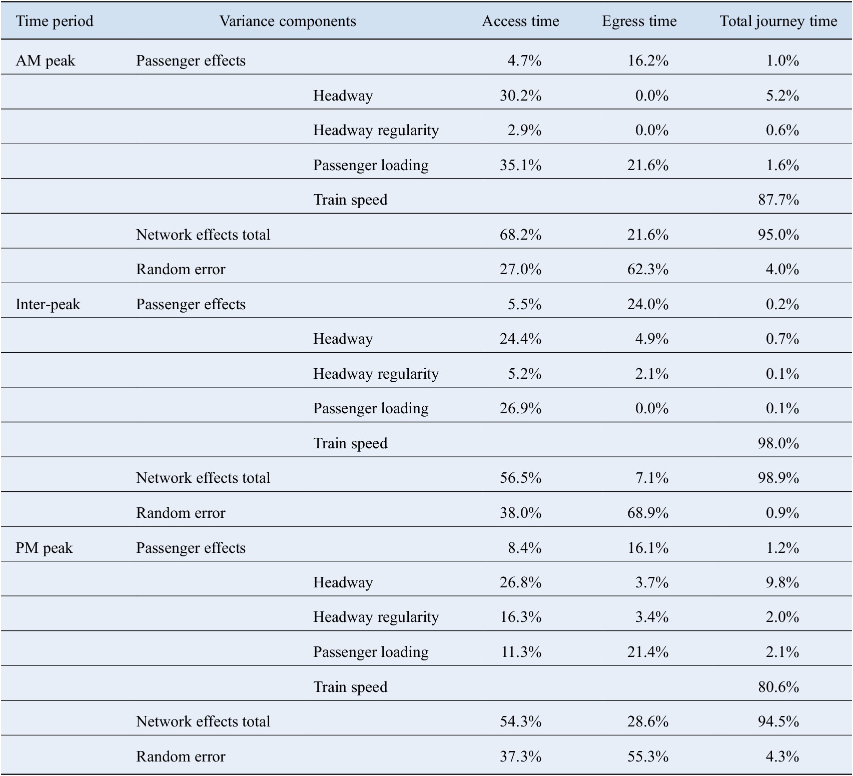

Figure 4. Proportion of variance represented by passenger effects by model.
The passenger effects capture the greatest proportion of variance in the egress time models, ranging from 16.1–24.0% of total variance across the different time periods. For the access time models, variance in passenger effects represents 4.7–8.4% of total variance. Passenger effects capture the least degree of variance in the total journey time models ranging from 0.2–1.2% of total variance.
When assessing the influence of the time of day, the results are mixed. For the egress time models, the passenger effects capture the greatest degree of variance in the inter-peak period at 24.0% of total variance in egress times. In the AM and PM peak, the proportion drops to approximately 16%. For the access time models, passenger effects represent similar proportions of variance in the AM peak (4.7%) and inter-peak periods (5.5%), and a relatively larger proportion of variance (8.4%) is captured in the PM peak. For the total journey time models, passenger effects capture the greatest degree of variance in the PM peak (1.2%), followed by the AM peak (1.0%), and inter-peak (0.2%).
The proportion of variance captured by passenger-level heterogeneity can be compared with the proportion of variance captured by the dynamic network effects. Figure 5 provides graphical illustrations of the comparisons. When considering journey times from tap-in to tap-out as a whole, the network characteristics capture the majority of variance ranging from 94.5–98.9%, while passenger heterogeneity represents a minimal 0.2–1.2%. Within the network effects category, train speeds (80.6–98.0%) capture the majority of variance, followed by train headways (0.7–9.8%), and passenger loading (0.1–2.1%). The results align with the elasticities of journey time previously presented, which indicate that train speed has the greatest influence on the magnitude of journey times with an average elasticity of −0.6, followed by train headways with an average elasticity of 0.07, and passenger loading with a combined average elasticity of 0.04. From the results, we can therefore conclude that operational characteristics represent the majority of variance in total journey times, and train speeds and headways have the greatest influence on the magnitude of journey times.

Figure 5. Comparison of variance components per model as proportion of total model variance.
For the access time models, network characteristics again represent the greatest proportion of variance ranging from 54.3–68.2% across all time periods, while passenger effects represent 4.7–8.4%. Of the network effects, headways (24.4–30.2%) and passenger loading (11.3–35.1%) represent the majority of variance. Unlike the access and total journey time models, the random error component represents the greatest degree of variance in egress times across all time periods, ranging from 55.3–68.9%. Of the systematic components, passenger effects are more influential, and network characteristics represent a lower proportion of variance compared to the access and total journey time models. In the inter-peak egress time model, passenger effects represent the greatest degree of variance at 24.0% while network effects, primarily headway, represent 7.1%. In the AM and PM peak models, network effects represent a greater proportion of variance at 21.6% and 28.6%, respectively, while passenger effects represent approximately 16% of variance. Of the network effects, passenger loading represents the greatest degree of variance (approximately 21%).
We can conclude that when considering variance in total journey times, train speeds and headways represent the majority of variance, while passenger effects represent a minimal proportion of variance, on average 1%. When analysing the access and egress time components in isolation, passenger effects are more influential. In the access time models, passenger effects represent on average 6% of variance in access times compared to an average 60% of variance represented by network characteristics. In the egress time models, passenger effects represent a similar or greater degree of variance as the dynamic network characteristics; averaged across all time periods, passenger effects and network effects equally represent 19% of variance.
5.4.2 As individual-specific realised values
The second interpretation involves treating the passenger effects as random intercepts. The model is interpreted in relation to the prediction of the realised value of the random effect for each individual passenger, which can be expressed as the best linear unbiased predictor:
 $$ {\displaystyle \begin{array}{l}E\left[\log \left({Y}_{ijt}\right)|\log \left({X}_{ijt}^{\prime}\right),{u}_i,{c}_j,{\gamma}_t\right],\\ {}\quad \mathrm{where}\ \log \left({Y}_{ijt}\right)\mid \log \left({X}_{ijt}^{\prime}\right),{u}_i,{c}_j,{\gamma}_t\sim \mathcal{N}\left(\alpha +\beta \log \left({X}_{ijt}^{\prime}\right)+{b}_{ijt}+{u}_i+{c}_j+{\gamma}_t,{\sigma}_{\varepsilon}^2+{\sigma}_b^2\right).\end{array}} $$
The realised values of passenger-specific effects represent inter-passenger effects. As per Equation (2), a passenger effect of magnitude
 $ {u}_i $
log-units represents a multiplicative increase of
$ {u}_i $
log-units represents a multiplicative increase of
 $ {e}^{u_i} $
units, which can be interpreted as an
$ {e}^{u_i} $
units, which can be interpreted as an
 $ \left({e}^{u_i}-1\right)\times 100\% $
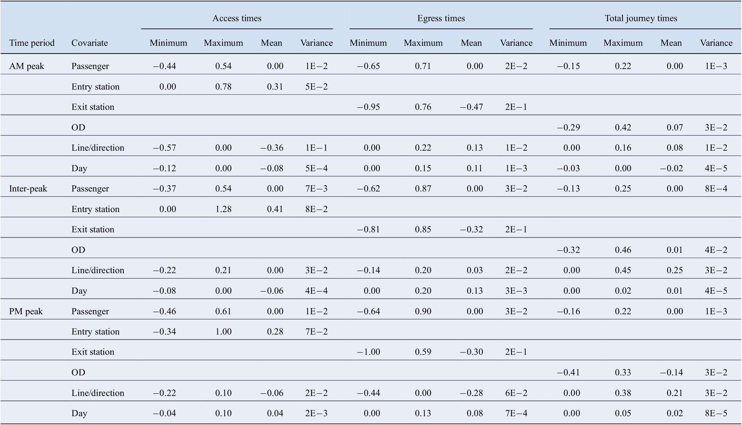
increase (or reduction) in the predicted values of journey times relative to free flow times. The same reasoning applies for the fixed effects, which capture group-specific effects related to days, stations, routes, and lines. The summary statistics for the realised values of the passenger effects and fixed effects are provided in Table 6, and kernel density distributions of the realised values of the passenger effects are illustrated in Figure 6.
$ \left({e}^{u_i}-1\right)\times 100\% $
increase (or reduction) in the predicted values of journey times relative to free flow times. The same reasoning applies for the fixed effects, which capture group-specific effects related to days, stations, routes, and lines. The summary statistics for the realised values of the passenger effects and fixed effects are provided in Table 6, and kernel density distributions of the realised values of the passenger effects are illustrated in Figure 6.
Table 6. Summary of realised values of passenger effects and fixed effects (log-units).
Abbreviation: OD, origin–destination.

Figure 6. Distribution of realized values of passenger effects by model.
Across all time periods, the passenger-specific effects for the egress time models range from a minimum effect of −0.65 log-units for the fastest passenger to a maximum effect of 0.90 log-units for the slowest passenger; this corresponds to a minimum 48% reduction to a maximum 145% increase in predicted egress times relative to free flow times. For the access time models, the individual effects range from a 37% reduction to a 85% increase in predicted access times, and for the total journey time models, the effects range from a 23% reduction to a 43% increase in predicted total journey times.
In terms of the influence of the time of day, the results are mixed. For access times, the range and variance of passenger effects are greatest during the PM peak followed by the AM peak and inter-peak, indicating that passenger effects have a greater influence on predicted access times during peak periods compared to the midday inter-peak. In the egress time models, the variance of passenger effects is similar across the time periods, while the range of passenger effects is greater during the PM peak and inter-peak compared to the AM peak. For the total journey time models, the range and variance of passenger effects are similar across the three time periods; the passenger effects cover the same magnitude of range during the AM peak and inter-peak, and a slightly narrower range during the PM peak.
The fixed effects capturing days and static network characteristics influence journey times at the same scale as the passenger-specific effects, i.e., at the scale of the predicted response. The passenger effects can be compared with the network fixed effects to give a general indication of whether passenger-specific or static network characteristics are more influential on predicted values of journey times (refer to Table 6 and Figure 7). In the total journey time models, the route and line/direction effects are generally more influential than the passenger effects, and day-specific effects are least influential. In the AM peak, when comparing the range of effects from the minimum to maximum outlying values, route-specific effects are the most influential, ranging from a minimum 25% reduction in journey times to a maximum 52% increase, followed by the passenger-specific effects ranging from a 14% reduction to a 24% increase. In the inter-peak and PM peak models, route effects are the most influential, ranging from a 34% reduction to a 59% increase in journey times, followed by line/direction effects ranging from a minimum no effect on journey times to a 57% increase, and passenger effects ranging from a 14% reduction to a 28% increase. When considering the variance and interquartile range of the effects, the route and line/direction effects are more influential compared to the middle 50% range of passenger effects.

Figure 7. Comparison of realized value of passenger effects and other network fixed effects by model.
In the access time models, when considering the range of effects from minimum to maximum values, station effects are the most influential group effect, followed by passenger effects, line/direction effects, and day effects. Station effects range from a minimum 29% reduction to a maximum 259% increase in access times, while passenger effects range from a minimum 37% reduction to a maximum 85% increase in access times. Discounting outliers and considering the interquartile ranges and variance of group effects, the line/direction effects and station effects are more influential when compared to the passenger effects for the middle 50% range of passengers.
When considering the range of effects for the egress time models, passenger effects are more influential, and have a similar or greater degree of influence than the station effects. In the AM and inter-peak, station effects range from a minimum reduction of 61% to a maximum increase of 134% in egress times, and passenger effects range from a minimum reduction of 48% to a maximum increase of 139% in egress times. In the PM peak, outlying passenger effects are more influential, ranging from a minimum reduction of 47% to a maximum increase of 145% while station effects range from a minimum reduction of 63% to a maximum increase of 80% in egress times. Considering variance and the interquartile ranges, the middle 50% of passenger effects are less influential than station effects but have a similar degree of influence to the line/direction effects.
In summary, when assessing the predicted values of journey time at a group-specific level, we can conclude that station and route-specific characteristics tend to have the greatest degree of influence on the magnitude of total journey times, followed by line/direction effects, passenger effects, and day effects. In the access and egress time models, passenger effects are relatively more influential. In the access time models, station effects are most influential, followed by passenger effects, which have a similar degree of influence, line/direction effects, and day effects. In the egress time models, the passenger-specific effects are equally or more influential than the station and line-specific characteristics.
6. Conclusions
In this paper, we seek to derive a more accurate characterisation of the underlying drivers of transit journey time variance, with a specific focus on separating the impact of passenger-specific effects from operational and physical characteristics of the network. Three lines on the London Underground metro system are analysed as a case study, and a random sample of passengers who undertake 10 or more repeat trips on the same OD route are selected. Twelve semiparametric regression models are generated; one for each component of journey time, namely access, on-train, and egress times, and total journey times over the AM peak, inter-peak, and PM peak.
The passenger-specific effects are statistically significant in the access, egress, and total journey time models across all time periods, however, the effects are not significant in the on-train time models. Two forms of interpretation are presented to assess the impact of passenger heterogeneity on journey times as follows: (i) the first interpretation involves using the variance component structure of the models to quantify the proportion of variance in journey times captured by intra-passenger heterogeneity, and (ii) the second interpretation involves extracting the realised values of the effects and treating these as passenger-specific intercepts to quantify inter-passenger effects on predicted journey times. The first interpretation relates to the comparison of passenger-specific effects with dynamic operational and demand characteristics, while the second interpretation relates to comparisons with physical static characteristics of the network.
When considering total passenger journey times from tap-in to tap-out, we find that dynamic operational and demand characteristics capture on average 96% of journey time variance, while passenger-level heterogeneity accounts for approximately 1%. Of the dynamic factors, train speeds and headways have the greatest influence on journey times. Comparing group-specific effects, we find that the fixed effects representing physical OD route characteristics are more influential than the passenger-specific effects. However, when taking into account passenger perceptions of travel, within the typically twice as onerous out-of-vehicle phases, passenger-level heterogeneity is found to be more influential. In terms of variance components, passenger-level heterogeneity represents on average 6% and 19% of variance, and network characteristics represent on average 60% and 19% of variance in the access and egress time models, respectively. As realised values, passenger-specific effects have a similar or greater degree of influence as the static station-specific characteristics. The results therefore show that while network-specific characteristics are the primary drivers of variance in journey times in absolute terms, a nontrivial proportion of passenger-perceived variance would be influenced by passenger-specific travel characteristics.
The estimates of passenger heterogeneity obtained in this analysis have potential applications related to improving the understanding of passenger movements within stations. The lower degree of passenger heterogeneity in the access models could arise from the walking speed and platform positioning constraints imposed on passengers to board the train as it arrives, while no such constraints are present in the egress phase. The result could also reflect a greater degree of way-finding complexity in terms of layout and/or station pedestrian flow control in the exiting direction at the destination stations. Second stage regression modelling of station characteristics could be undertaken to disentangle station complexity from inherent passenger characteristics.
A number of other future research areas could also be explored. The analysis could be applied at a more disaggregate level to quantify passenger heterogeneity at a station or route-specific level. The degree of passenger heterogeneity across the stations or routes could be compared, and those exhibiting a greater degree of heterogeneity could potentially indicate a greater degree of way-finding complexity. Second stage modelling of disaggregate station characteristics could then disentangle inherent passenger characteristics from operational and physical station characteristics, and guide operators in identifying station elements that require potential improvements. In terms of the type of passengers analysed in this study, the models focus on the behaviour of a sample of passengers who undertake 10 or more trips only. A wider range of passengers could be sampled to obtain a more comprehensive set of results across different passenger demographics. Finally, the models could be scaled up to a network level, and with additional data on different networks, comparisons of the impact of passenger heterogeneity across networks could be made.
Acknowledgments
The authors would like to thank Transport for London (TfL) for providing the data used in the analysis. It should be noted that any opinions, findings, and conclusions or recommendations expressed in this material are those of the authors and do not necessarily reflect the views of TfL.
Funding Statement
This research was jointly funded by TfL and the Transport Strategy Centre (TSC) at Imperial College London.
Competing Interests
The authors declare no competing interests exist.
Data Availability Statement
The data used in this study were accessed under a confidentiality agreement with TfL. Restrictions apply to the availability of these data, and permissions must be sought from TfL for access to the data.
Author Contributions
Conceptualisation: D.J.G., R.J.A., and R.S.; Methodology: D.J.G. and R.S.; Formal analysis: R.S. and D.J.G.; Data curation: R.S.; Writing-original draft: R.S. and D.J.G.; Writing-review and editing: R.S. and D.J.G.; Supervision: D.J.G. and R.J.A.; Funding acquisition: D.J.G. and R.J.A.
Appendices
B. Regression Modelling Results
Table B1. Model form 1 goodness-of-fit statistics—final model form with all continuous covariates modelled with nonparametric smooths, fixed network effects, and random passenger effects.
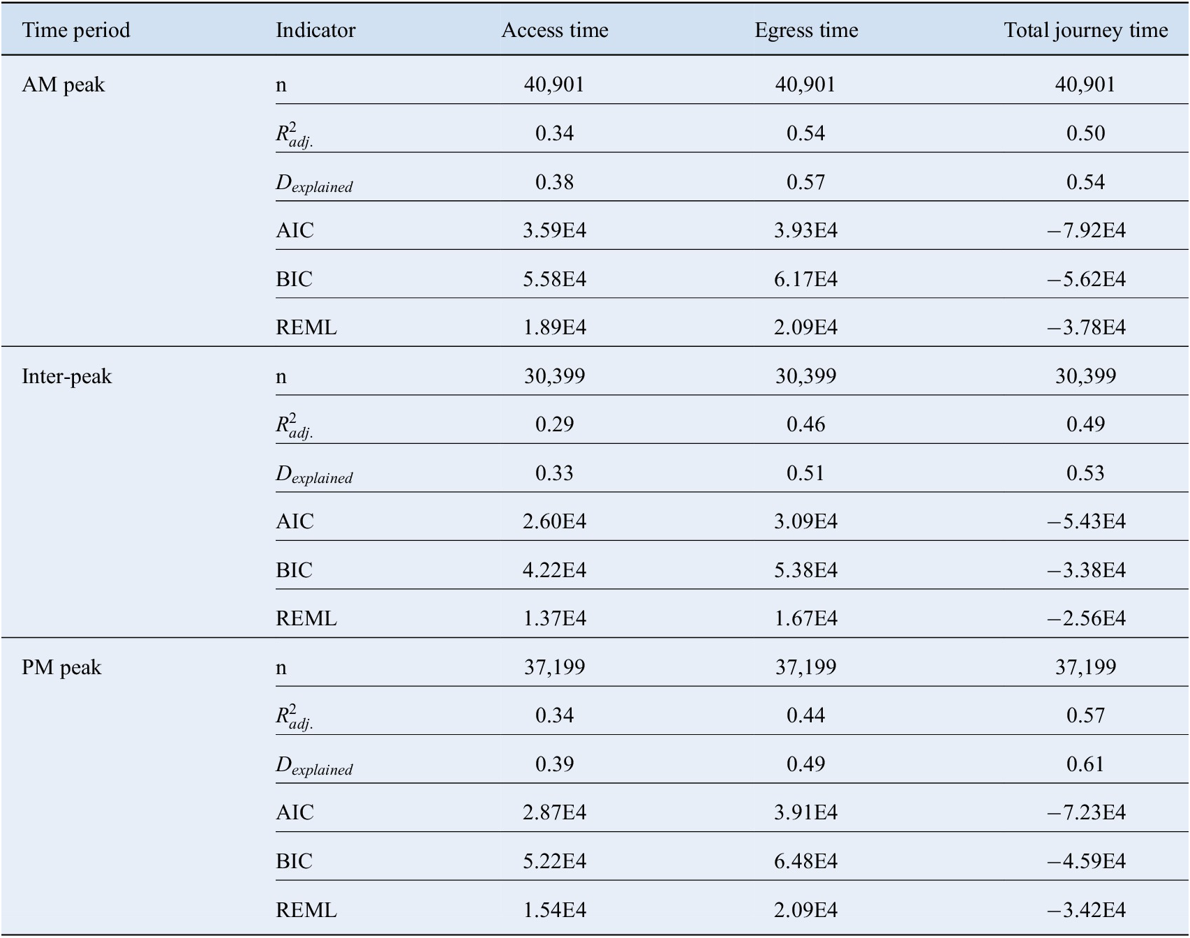
Abbreviations: AIC, Akaike Information Criterion;
 $ {D}_{explained} $
, deviance explained;
$ {D}_{explained} $
, deviance explained;
 $ n $
, number of observations;
$ n $
, number of observations;
 $ {R}_{adj.}^2 $
, adjusted coefficient of determination; REML, restricted maximum likelihood.
$ {R}_{adj.}^2 $
, adjusted coefficient of determination; REML, restricted maximum likelihood.
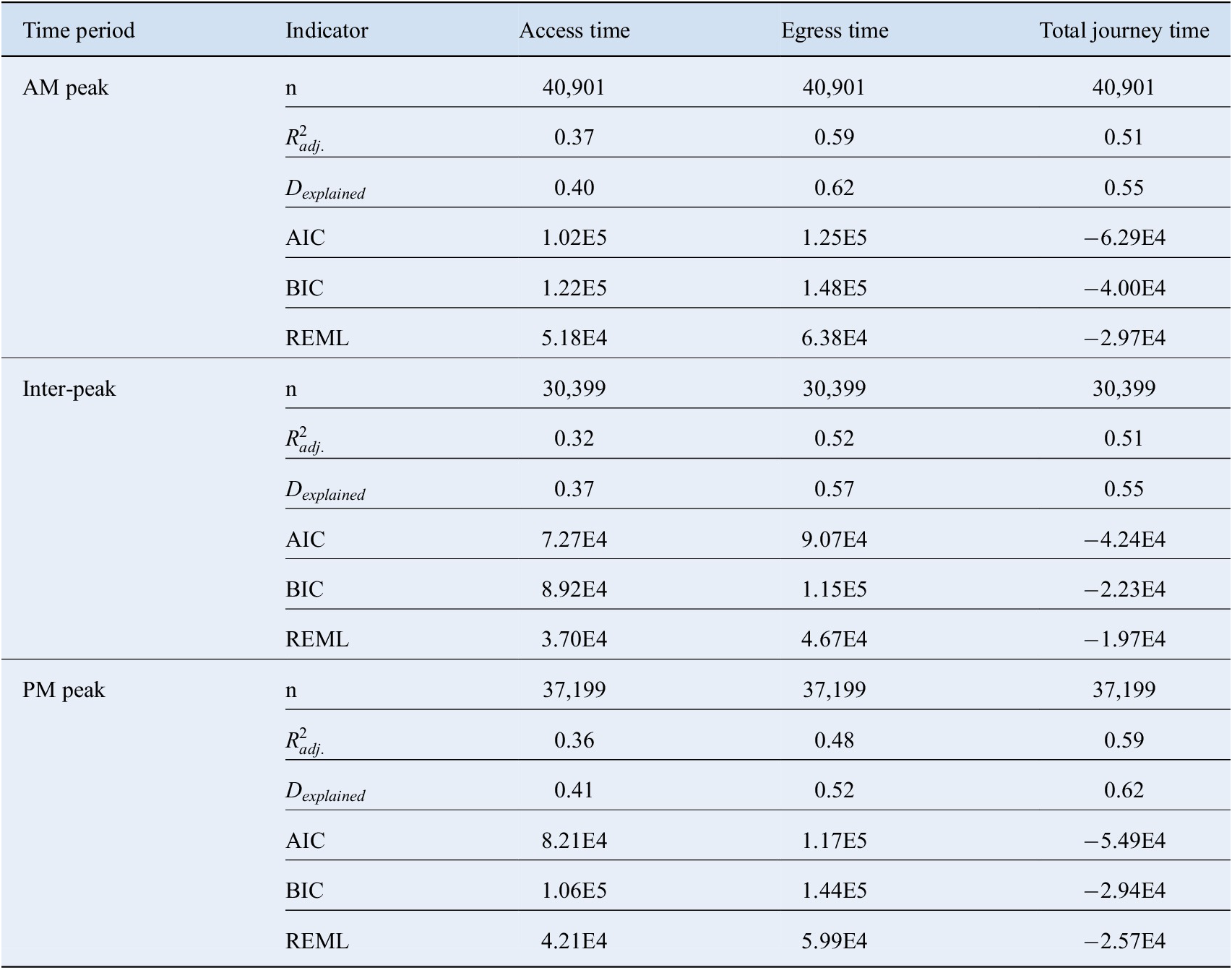
Table B2. Model form 2 goodness-of-fit statistics—all continuous covariates modelled with nonparametric smooths, fixed network effects, and fixed passenger effects.

Abbreviations: AIC, Akaike Information Criterion;
 $ {D}_{explained} $
, deviance explained;
$ {D}_{explained} $
, deviance explained;
 $ n $
, number of observations;
$ n $
, number of observations;
 $ {R}_{adj.}^2 $
, adjusted coefficient of determination; REML, restricted maximum likelihood.
$ {R}_{adj.}^2 $
, adjusted coefficient of determination; REML, restricted maximum likelihood.
Table B3. Model form 3 goodness-of-fit statistics—Equivalent to final model form but no log-transformation.
Abbreviations: AIC, Akaike Information Criterion;
 $ {D}_{explained} $
, deviance explained;
$ {D}_{explained} $
, deviance explained;
 $ n $
, number of observations;
$ n $
, number of observations;
 $ {R}_{adj.}^2 $
, adjusted coefficient of determination; REML, restricted maximum likelihood.
$ {R}_{adj.}^2 $
, adjusted coefficient of determination; REML, restricted maximum likelihood.
Table B4. Model form 4 goodness-of-fit statistics—Linear continuous covariates, no group-specific effects.

Abbreviations: AIC, Akaike Information Criterion;
 $ {D}_{explained} $
, deviance explained;
$ {D}_{explained} $
, deviance explained;
 $ n $
, number of observations;
$ n $
, number of observations;
 $ {R}_{adj.}^2 $
, adjusted coefficient of determination; REML, restricted maximum likelihood.
$ {R}_{adj.}^2 $
, adjusted coefficient of determination; REML, restricted maximum likelihood.


 Open access
Comments
No Comments have been published for this article.