Introduction
In Reference Mayor and Queloz1995, Mayor & Queloz detected the first exoplanet orbiting a Sun-like star. This was just the first of many, and 10 years later more than 150 exoplanets were already known. It was at that time that a planet with a mass lower than 0.10 M ⊕ was found orbiting the low-mass star GJ 876 (Rivera et al. Reference Rivera, Lissauer and Butler2005). This was the first ‘Earth-sized’ planet to be found, also called ‘Super-Earth’.
This new class of planets with mass lower than 10 M ⊕, is believed to have an icy/rocky core surrounded by a dense gaseous envelope (Alibert et al. Reference Alibert, Baraffe and Benz2006). As an example, for a planet with a mass of 8 M ⊕, Rafikov (Reference Rafikov2006) showed that ~87.5% of its mass may be made of rock, whereas ~12.5% may be an H2–He gaseous envelope. We may compare these results with the values of the planet Earth, whose atmosphere represents only 0.0001% of the total mass, and for Venus, whose atmosphere/mass ratio is 0.01%.
There are many differences between the so-called ‘Super-Earths’ and the telluric planets of the Solar System, and also much to be discovered about these new worlds. Still, the use of our knowledge on the telluric planets to study the properties of similar exoplanets is of major interest. In particular, because some of these planets may be orbiting in the habitable zone (HZ) (see, e.g., Udry et al. Reference Udry, Bonfils and Delfosse2007), the study of their spin evolution to infer their possible climate becomes important in the search of life elsewhere in the Universe. Although most of these planets will be quite different from the Earth, in the remaining of the paper, the term Earth-sized planet denotes a planet with mass smaller than 10 M ⊕ orbiting in the vicinity of the HZ or closer to their parent star.
The HZ is defined as a range of distance to the star where the insolation received by an Earth-sized planet is adequate to allow its surface to maintain liquid water (Kasting et al. Reference Kasting, Whitmire and Reynolds1993; Kopparapu et al. Reference Kopparapu, Ramirez and Kasting2013a, Reference Kopparapu, Ramirez and Kastingb). But to say that a planet is in the HZ is not the same as to say a planet is habitable. There are other factors, such as the obliquity, eccentricity, atmosphere composition or tidal effects that should also be considered when assessing habitability.
Several efforts have been made to explore these and other factors that may contribute to the habitability of an exoplanet. As an example, Barnes et al. (Reference Barnes, Mullins and Goldblatt2013) show that tidal heating can induce a runaway greenhouse on explanets orbiting low-mass stars, which may cause all the hydrogen to escape, and so may all the water. On the other hand, modelling by Barnes et al. (Reference Barnes, Raymond, Jackson and Greenberg2008) shows that Earth-sized exoplanets orbiting in the HZ of an M-dwarf can support life. These planets may have strong enough magnetic fields that might protect their atmospheres and surfaces. But to infer about the habitability of a planet, there is an effect that should not be neglected: tidal dissipation. Tidal interactions will contribute to the planetary spin evolution, having an impact on the final obliquity, spin rate and eccentricity (e.g., Heller et al. Reference Heller, Leconte and Barnes2011).
Since Earth-sized exoplanets are believed to have dense atmospheres, when studying their spin evolution, we have to consider two kinds of tidal effects: the traditional bodily tides of gravitational origin (gravitational tides), but also thermal atmospheric tides. The former tends to despin the planet, while the latter may counteract the gravitational tidal effect on the planet's rotation (Gold & Soter Reference Gold and Soter1969). In the Solar System, Venus and the Earth are the only telluric planets having a significant atmosphere. From these two, only Venus is believed to have reached a final equilibrium rotation rate (Dobrovolskis Reference Dobrovolskis1980; Correia & Laskar Reference Correia and Laskar2001, Reference Correia and Laskar2003b). As all known Earth-sized exoplanets are closer to the parent star than Venus is to the Sun, it is expected that they have also reached rotational equilibrium (Laskar & Correia Reference Laskar and Correia2004; Correia et al. Reference Correia, Levrard and Laskar2008). Therefore, their environments are probably more similar to Venus than to the Earth. We can thus use the model developped for the undestanding of the spin evolution of Venus (Correia et al. Reference Correia, Laskar and Néron de Surgy2003; Correia & Laskar Reference Correia and Laskar2003b) for investigating the possible spin evolution of the Earth-sized exoplanets.
In this work, we expect to be able to infer about the present rotation of Earth-sized planets. Unlike Venus, whose orbit is almost circular, most of these exoplanets have non-zero eccentricities. Thus, the above-mentioned model for Venus’ rotation needs to be generalized in order to include the effect of the orbital eccentricity. We also assess if these planets can only evolve to final obliquity of 0° and 180° (Correia et al. Reference Correia, Laskar and Néron de Surgy2003), or if they can present intermediate stable obliquities. In the ‘Equations of motion' section, we present the equations of motion that describe the long-term spin evolution of a terrestrial planet. We also describe the contribution of the main dissipative effects: the gravitational tides, thermal atmospheric tides and core–mantle friction. In the ‘Dynamical analysis’, we present a dynamical analysis for the spin evolution and for the final equilibrium rotation states. In the ‘Numerical simulations’, we present numerical simulations for the spin evolution starting with different initial rotation periods and obliquities. We apply our model to the known Earth-sized planets as well as fictitious Earth-sized planets in the HZ of Sun-like stars. We end this study by presenting our conclusions in the final section.
Equations of motion
Conservative motion
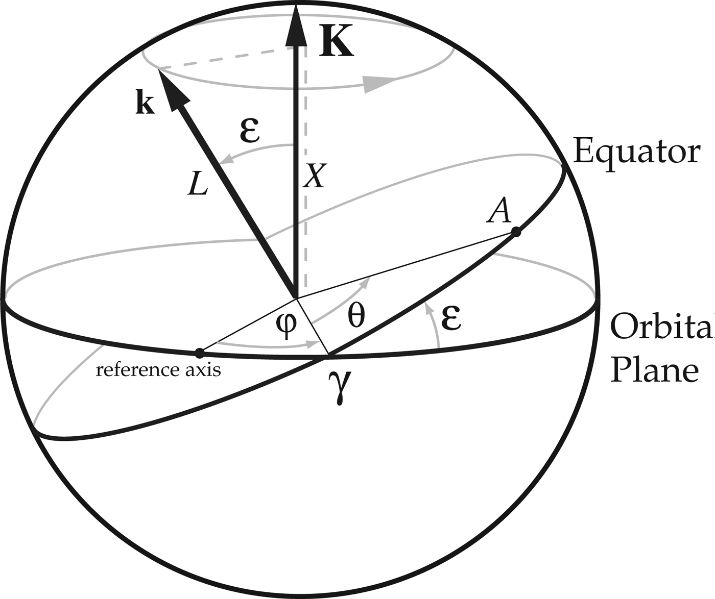
The Hamiltonian of the motion can be written using the classical canonical Andoyer's action and angle variables (Andoyer Reference Andoyer1923; Kinoshita Reference Kinoshita1977), but these variables become degenerate due to a simplifying assumption that is done here: the planet is considered to be a rigid body with moments of inertia A=B<C, and we merge the figure axis with the direction of the angular momentum (gyroscopic approximation)Footnote 1. We are then left with only two action variables (L, X) and their conjugate angles (θ, φ) (Néron de Surgy & Laskar Reference Néron de Surgy and Laskar1997)Footnote 2. The quantity L=Cω, with rotation rate ω, is the the angular momentum along the C-axis, and X=L cos ε, where ε is the obliquity, is its projection on the normal to the quasi-inertial ecliptic plane. The variable θ is the hour angle between the equinox and a fixed point of the equator, and φ is the precession angle (Fig. 1). Averaging the Hamiltonian over the rotation angle and the mean anomaly, we getFootnote 3 (Kinoshita Reference Kinoshita1977; Néron de Surgy & Laskar Reference Néron de Surgy and Laskar1997; Correia & Laskar Reference Correia and Laskar2010b)
 $$\bar H = \displaystyle{{L^2} \over {2C}} - {\rm \alpha} \displaystyle{{X^2} \over {2L}}\;, $$
where
 $${\rm \alpha} = \displaystyle{{3GM_*} \over {2a^3 (1 - e^2 )^{3/2}}} \displaystyle{{E_{\rm d}} \over {\rm \omega}} \simeq \displaystyle{3 \over 2}\displaystyle{{n^2} \over {\rm \omega}} \left( {1 + \displaystyle{3 \over 2}e^2} \right)E_{\rm d} $$
is the ‘precession constant’, while quantities G, M *, a, n and e are the gravitational constant, stellar mass, semi-major axis, mean motion and eccentricity, respectively. Quantity E d is the dynamical ellipticityFootnote 4,
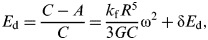 $$E_{\rm d} = \displaystyle{{C - A} \over C} = \displaystyle{{k_{\rm f} R^5} \over {3GC}}{\rm \omega} ^2 + {\rm \delta} E_{\rm d}, $$
where R is the planet radius, and k f is the fluid Love number. The first part of this expression corresponds to the flattening in hydrostatic equilibrium (Lambeck Reference Lambeck1980), and the second corresponds to the departure from this equilibrium.

Fig. 1. Andoyer's canonical variables. L is the projection of the total rotational angular momentum vector L on the principal axis of inertia k, and X the projection of the angular momentum vector on the normal to the orbit K. The angle between the line of nodes γ and a fixed point of the equator A is the hour angle, θ, whereas the angle between a reference point in the orbit and the line of nodes γ is the precession angle, φ.
Since Andoyer's variables are canonical, the spin equations of motion are easily obtained from the mean Hamiltonian (equation (1)) as
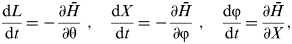 $$\displaystyle{{{\rm d}L} \over {{\rm d}t}} = - \displaystyle{{{\rm \partial} \bar H} \over {\partial {\rm \theta}}} \;, \quad \displaystyle{{{\rm d}X} \over {{\rm d}t}} = - \displaystyle{{\partial \bar H} \over {\partial {\rm \varphi}}} \;, \quad \displaystyle{{{\rm d}{\rm \varphi}} \over {{\rm d}t}} = \displaystyle{{\partial \bar H} \over {\partial X}},$$
which gives
 $$\displaystyle{{{\rm d}L} \over {{\rm d}t}} = \displaystyle{{{\rm d}X} \over {{\rm d}t}} = 0,\quad {\rm and}\quad \displaystyle{{{\rm d}{\rm \varphi}} \over {{\rm d}t}} = - {\rm \alpha} \cos {\rm \varepsilon}, $$
i.e., the rotation rate and the obliquity are constant, and the planet precesses at a constant rate.
Tidal effects
Tidal effects arise from planetary differential and inelastic deformations caused by a perturbing body. There are two types of tidal effects: the gravitational tides and the thermal atmospheric tides. The estimations for both effects are based on a general formulation of the tidal potential, initiated by Darwin (Reference Darwin1880).
Gravitational tides
Gravitational tides are raised on the planet by a perturbing body because of the gravitational gradient across the planet. The force experienced by the side facing the perturbing body is stronger than that experienced by the far side. These tides are mainly important upon the solid (or liquid) part of the planet, and are independent of the existence of an atmosphere.
Since the planets are not perfectly rigid, there is a distortion that gives rise to a tidal bulge. This redistribution of mass modifies the gravitational potential generated by the planet in any point of the space. The additional amount of potential, the tidal potential U g, is responsible for the modifications in the planet's spin (and orbit), and it is given byFootnote 5 (e.g., Lambeck Reference Lambeck1980):
 $$U_{\rm g} = - k_2 \displaystyle{{GM_*^2} \over R}\left( {\displaystyle{R \over {r_*}}} \right)^3 \left( {\displaystyle{R \over r}} \right)^3 P_2 (\cos \,S),$$
where r and r * are the distances from the planet's centre of mass to a generic point and to the star, respectively, S is the angle between these two directions, P 2 are the second-order Legendre polynomials, and k 2 is the second potential Love number.
Expressing the tidal potential given by expression (6) in terms of Andoyer angles (θ, φ), we can obtain the contribution to the spin evolution from expressions (4) using U g at the place of  ${\overline {\cal H}}$. As we are interested here in the study of the secular evolution of the spin, we also average U g over the periods of mean anomaly and longitude of the periapse of the orbit. This work is done with the help of the algebraic manipulator TRIP (Laskar Reference Laskar1989, Reference Laskar1994), which expands the potential in Fourier series, as in Kaula (Reference Kaula1964) and Correia & Laskar (Reference Correia and Laskar2010b). For a planet orbiting its host star, where the star is both the perturbing and interacting body (r=r *), we then find for the averaged equations of motion:
 $$\displaystyle{{{\rm d}L} \over {{\rm d}t}} = K_{\rm g} \mathop \sum \limits_{\rm \sigma} b_{\rm g} ({\rm \sigma} ){\rm \Lambda} _{\rm \sigma} ^{\rm g} (x,e),$$
 $$\displaystyle{{{\rm d}X} \over {{\rm d}t}} = K_{\rm g} \mathop \sum \limits_{\rm \sigma} b_{\rm g} ({\rm \sigma} ){\rm \Upsilon} _{\rm \sigma} ^{\rm g} (x,e),$$
where
 $$K_{\rm g} = - \displaystyle{{GM_*^2 R^5} \over {a^6}}, $$
and x=X/L=cos ε. The coefficients, Λσg and  ${\rm \Upsilon} _{\rm \sigma} ^{\rm g} $, are polynomials in the eccentricity (Kaula Reference Kaula1964). For a planet with moderate eccentricity, we may neglect terms in e 4 and greater, and obtain the following expansion for the previous equations:
$$\eqalign{\displaystyle{1 \over {K_{\rm g}}} \displaystyle{{{\rm d}L} \over {{\rm d}t}} = & b_{\rm g} (2{\rm \omega} + 3n)\displaystyle{{147} \over {128}}e^2 (1 - x)^4 \cr & + b_{\rm g} (2{\rm \omega} + 2n)\displaystyle{3 \over {32}}(1 - 5e^2 )(1 - x)^4 \cr & + b_{\rm g} (2{\rm \omega} + n)\displaystyle{3 \over {128}}e^2 (37 + 70x + 37x^2 )(1 - x)^2 \cr & + b_{\rm g} (2{\rm \omega} )\displaystyle{3 \over 8}(1 + 3e^2 )(1 - x^2 )^2 \cr & + b_{\rm g} (2{\rm \omega} - n)\displaystyle{3 \over {128}}e^2 (37 - 70x + 37x^2 )(1 + x)^2 \cr & + b_{\rm g} (2{\rm \omega} - 2n)\displaystyle{3 \over {32}}(1 - 5e^2 )(1 + x)^4 \cr & + b_{\rm g} (2{\rm \omega} - 3n)\displaystyle{{147} \over {128}}e^2 (1 + x)^4 \cr & + b_{\rm g} ({\rm \omega} + 3n)\displaystyle{{147} \over {64}}e^2 (1 - x^2 )(1 - x)^2 \cr & + b_{\rm g} ({\rm \omega} + 2n)\displaystyle{3 \over {16}}(1 - 5e^2 )(1 - x^2 )(1 - x)^2 \cr & + b_{\rm g} ({\rm \omega} + n)\displaystyle{3 \over {64}}e^2 (1 - 2x + 37x^2 )(1 - x^2 ) \cr & + b_{\rm g} ({\rm \omega} )\displaystyle{3 \over 4}(1 + 3e^2 )(1 - x^2 )x^2 \cr & + b_{\rm g} ({\rm \omega} - n)\displaystyle{3 \over {64}}e^2 (1 + 2x + 37x^2 )(1 - x^2 ) \cr & + b_{\rm g} ({\rm \omega} - 2n)\displaystyle{3 \over {16}}(1 - 5e^2 )(1 - x^2 )(1 + x)^2 \cr & + b_{\rm g} ({\rm \omega} - 3n)\displaystyle{{147} \over {64}}e^2 (1 - x^2 )(1 + x)^2,} $$and
$$\eqalign{\displaystyle{1 \over {K_{\rm g}}} \displaystyle{{{\rm d}X} \over {{\rm d}t}} = & - b_{\rm g} (2{\rm \omega} + 3n)\displaystyle{{147} \over {128}}e^2 (1 - x)^4 \cr & - b_{\rm g} (2{\rm \omega} + 2n)\displaystyle{3 \over {32}}(1 - 5e^2 )(1 - x)^4 \cr & - b_{\rm g} (2{\rm \omega} + n)\displaystyle{3 \over {128}}e^2 (1 - x)^4 \cr & + b_{\rm g} (2{\rm \omega} - n)\displaystyle{3 \over {128}}e^2 (1 + x)^4 \cr & + b_{\rm g} (2{\rm \omega} - 2n)\displaystyle{3 \over {32}}(1 - 5e^2 )(1 + x)^4 \cr & + b_{\rm g} (2{\rm \omega} - 3n)\displaystyle{{147} \over {128}}e^2 (1 + x)^4 \cr & - b_{\rm g} ({\rm \omega} + 3n)\displaystyle{{147} \over {32}}e^2 (1 - x^2 )(1 - x)^2 \cr & - b_{\rm g} ({\rm \omega} + 2n)\displaystyle{3 \over 8}(1 - 5e^2 )(1 - x^2 )(1 - x)^2 \cr & - b_{\rm g} ({\rm \omega} + n)\displaystyle{3 \over {32}}e^2 (1 - x^2 )(1 - x)^2 \cr & + b_{\rm g} ({\rm \omega} - n)\displaystyle{3 \over {32}}e^2 (1 - x^2 )(1 + x)^2 \cr & + b_{\rm g} ({\rm \omega} - 2n)\displaystyle{3 \over 8}(1 - 5e^2 )(1 - x^2 )(1 + x)^2 \cr & + b_{\rm g} ({\rm \omega} - 3n)\displaystyle{{147} \over {32}}e^2 (1 - x^2 )(1 + x)^2 \cr & - b_{\rm g} (3n)\displaystyle{{441} \over {64}}e^2 (1 - x^2 )^2 \cr & - b_{\rm g} (2n)\displaystyle{9 \over {16}}(1 - 5e^2 )(1 - x^2 )^2 \cr & - b_{\rm g} (n)\displaystyle{9 \over {64}}e^2 (1 - x^2 )^2.} $$The coefficients b g(σ) are related to the dissipation of the mechanical energy of tides in the planet's interior, responsible for a time delay Δt g(σ) between the position of ‘maximal tide’ and the sub-stellar point. They are related to the geometric lag δg(σ) as:
 $$b_{\rm g} ({\rm \sigma} ) = k_2 \sin {\rm \;} 2{\rm \delta} _{\rm g} ({\rm \sigma} ) = k_2 \sin ({\rm \sigma} {\rm \Delta} t_{\rm g} ({\rm \sigma} )).$$
Dissipation equations (10) and (11) must be invariant under the transformation (ω, x) by (−ω, −x) which implies that b(σ)=−b(−σ). That is, b(σ) is an odd function of σ (Correia et al. Reference Correia, Laskar and Néron de Surgy2003). Although mathematically equivalent, the couples (ω, x) and (−ω,−x) correspond to two different physical situations (see Correia & Laskar Reference Correia and Laskar2001).
Thermal atmospheric tides
The differential absorption of the Solar heat by the planet's atmosphere gives rise to local variations of temperature and consequently to pressure gradients. The mass of the atmosphere is then permanently redistributed, adjusting for an equilibrium position. More precisely, the particles of the atmosphere move from the high-temperature zone (at the sub-solar point) to the low-temperature areas (e.g., Arras & Socrates Reference Arras and Socrates2010). Observations on Earth show that the pressure redistribution is essentially a superposition of two pressure waves: a diurnal tide of small amplitude and a strong semi-diurnal tide (Bartels Reference Bartels1932; Haurwitz Reference Haurwitz1964; Chapman & Lindzen Reference Chapman and Lindzen1970).
As for gravitational tides, the redistribution of mass in the atmosphere gives rise to an atmospheric bulge that modifies the gravitational potential generated by the atmosphere in any point of the space. The tidal potential U a responsible for the spin changes is given byFootnote 6 (e.g., Correia & Laskar Reference Correia and Laskar2003a):
 $$U_{\rm a} = - \displaystyle{3 \over 5}\displaystyle{{\tilde p_2} \over {{\rm \bar \rho}}} \left( {\displaystyle{R \over r}} \right)^3 P_2 (\cos \,S),$$
where  $\tilde p_2 $ is the second-order surface pressure variations, and ${\rm \bar \rho} $ is the mean density of the planet.
To find the contributions to the spin we use expressions (4) together with the averaging method over fast varying angles (mean anomaly and longitude of the periapse), which gives:
 $$\displaystyle{{{\rm d}L} \over {{\rm d}t}} = K_{\rm a} \mathop \sum \limits_{\rm \sigma} b_{\rm a} ({\rm \sigma} ){\rm \Lambda} _{\rm \sigma} ^{\rm a} (x,e),$$
 $$\displaystyle{{{\rm d}X} \over {{\rm d}t}} = K_{\rm a} \mathop \sum \limits_{\rm \sigma} b_{\rm a} ({\rm \sigma} ){\rm \Upsilon} _{\rm \sigma} ^{\rm a} (x,e),$$
where
 $$K_{\rm a} = - \displaystyle{{3M_* R^3} \over {5{\rm \bar \rho} a^3}}. $$
The b a(σ) factor is now:
 $$\eqalign{b_{\rm a} ({\rm \sigma} )& = \tilde p_2 ({\rm \sigma} )\sin {\rm \;} \left( {{\rm \sigma} {\rm \Delta} t_{\rm a} ({\rm \sigma} )} \right) = \tilde p_2 ({\rm \sigma} )\sin {\rm \;} 2{\rm \delta} _{\rm a} ({\rm \sigma} ) \cr & = |\tilde p_2 |\sin 2({\rm \delta} _{\rm a} ({\rm \sigma} ) + {\rm \pi} /2) = - |\tilde p_2 |\sin 2{\rm \delta} _{\rm a} ({\rm \sigma} ),} $$
where Δt a is the atmosphere's delayed response to the stellar heat excitation, and δa is the corresponding geometric lag. The amplitude of the bulge,  $\tilde p_2 $, is the second-order surface pressure variations (Chapman & Lindzen Reference Chapman and Lindzen1970):
 $$\tilde p_2 ({\rm \sigma} ) = {\rm i}\displaystyle{\gamma \over {\rm \sigma}} \tilde p_0 \left( {\nabla \cdot {\bf \upsilon} _{\rm \sigma} - \displaystyle{{{\rm \gamma} - 1} \over {\rm \gamma}} \displaystyle{{J_{\rm \sigma}} \over {gH_0}}} \right) = {\rm i}\displaystyle{{{\rm {\cal P}}_{\rm \sigma}} \over {\rm \sigma}}, $$
where γ=7/5 for a perfect diatomic gas,  $\tilde p_0 $ is the mean surface pressure, υσ is the tidal winds velocity, J σ is the amount of heat absorbed or emitted by unit of mass of air per unit time, and H 0 is the scale height at the surface. The imaginary number in equation (18) causes the pressure variations to lead the star (i=eiπ/2).
The coefficients Λσa and  ${\rm \Upsilon} _{\rm \sigma} ^{\rm a} $ are also polynomials in the eccentricity, but different from their analogues for gravitational tides (equations (10) and (11)). However, for zero eccentricity they become equal, i.e., Λσa(e=0)=Λσg(e=0), and ${\rm \Upsilon} _{\rm \sigma} ^{\rm a} (e = 0) = {\rm \Upsilon} _{\rm \sigma} ^{\rm g} (e = 0)$. Once more, for a planet with moderate eccentricity, we can neglect terms in e 4 and greater, and obtain the following expansion for equations (14) and (15):
$$\eqalign{\displaystyle{1 \over {K_{\rm a}}} \displaystyle{{{\rm d}L} \over {{\rm d}t}} =\ & b_{\rm a} (2{\rm \omega} + 3n)e^2 \displaystyle{{27} \over {32}}(1 - x)^4 \cr & + b_{\rm a} (2{\rm \omega} + 2n)\displaystyle{3 \over {32}}(1 - 3e^2 )(1 - x)^4 \cr & - b_{\rm a} (2{\rm \omega} + n)e^2 \displaystyle{3 \over {32}}(1 - x)^4 \cr & + b_{\rm a} (2{\rm \omega} )\displaystyle{3 \over 8}(1 + 5e^2 )(1 - x^2 )^2 \cr & - b_{\rm a} (2{\rm \omega} - n)e^2 \displaystyle{3 \over {32}}(1 + x)^4 \cr & + b_{\rm a} (2{\rm \omega} - 2n)\displaystyle{3 \over {32}}(1 - 3e^2 )(1 + x)^4 \cr & + b_{\rm a} (2{\rm \omega} - 3n)e^2 \displaystyle{{27} \over {32}}(1 + x)^4 \cr & + b_{\rm a} ({\rm \omega} + 3n)e^2 \displaystyle{{27} \over {16}}(1 - x^2 )(1 - x)^2 \cr & + b_{\rm a} ({\rm \omega} + 2n)\displaystyle{3 \over {16}}(1 - 3e^2 )(1 - x^2 )(1 - x)^2 \cr & - b_{\rm a} ({\rm \omega} + n)e^2 \displaystyle{3 \over {16}}(1 - x^2 )(1 - x)^2 \cr & + b_{\rm a} ({\rm \omega} )\displaystyle{3 \over 4}(1 + 5e^2 )x^2 (1 - x^2 ) \cr & - b_{\rm a} ({\rm \omega} - n)e^2 \displaystyle{3 \over {16}}(1 - x^2 )(1 + x)^2 \cr & + b_{\rm a} ({\rm \omega} - 2n) \displaystyle{3 \over {16}}(1 - 3e^2 )(1 - x^2 )(1 + x)^2 \cr & + b_{\rm a} ({\rm \omega} - 3n)e^2 \displaystyle{{27} \over {16}}(1 - x^2 )(1 + x)^2,} $$and
$$\eqalign{\displaystyle{1 \over {K_{\rm a}}} \displaystyle{{{\rm d}X} \over {{\rm d}t}} = & - b_{\rm a} (2{\rm \omega} + 3n)e^2 \displaystyle{{27} \over {32}}(1 - x)^4 \cr & - b_{\rm a} (2{\rm \omega} + 2n)\displaystyle{3 \over {32}}(1 - 3e^2 )(1 - x)^4 \cr & + b_{\rm a} (2{\rm \omega} + n)e^2 \displaystyle{3 \over {32}}(1 - x)^4 \cr & - b_{\rm a} (2{\rm \omega} - n)e^2 \displaystyle{3 \over {32}}(1 + x)^4 \cr & + b_{\rm a} (2{\rm \omega} - 2n)\displaystyle{3 \over {32}}(1 - 3e^2 )(1 + x)^4 \cr & + b_{\rm a} (2{\rm \omega} - 3n)e^2 \displaystyle{{27} \over {32}}(1 + x)^4 \cr & - b_{\rm a} ({\rm \omega} + 3n)e^2 \displaystyle{{27} \over 8}(1 - x^2 )(1 - x)^2 \cr & - b_{\rm a} ({\rm \omega} + 2n)\displaystyle{3 \over 8}(1 - 3e^2 )(1 - x^2 )(1 - x)^2 \cr & + b_{\rm a} ({\rm \omega} + n)e^2 \displaystyle{3 \over 8}(1 - x^2 )(1 - x)^2 \cr & - b_{\rm a} ({\rm \omega} - n)e^2 \displaystyle{3 \over 8}(1 - x^2 )(1 + x)^2 \cr & + b_{\rm a} ({\rm \omega} - 2n)\displaystyle{3 \over 8}(1 - 3e^2 )(1 - x^2 )(1 + x)^2 \cr & + b_{\rm a} ({\rm \omega} - 3n)e^2 \displaystyle{{27} \over 8}(1 - x^2 )(1 + x)^2 \cr & - b_{\rm a} (3n)e^2 \displaystyle{{81} \over {16}}(1 - x^2 )^2 \cr & - b_{\rm a} (2n)\displaystyle{9 \over {16}}(1 - 3e^2 )(1 - x^2 )^2 \cr & + b_{\rm a} (n)e^2 \displaystyle{9 \over {16}}(1 - x^2 )^2.} $$Neglecting the tidal winds υσ, from expression (18) we have
 $${\rm {\cal P}}_{\rm \sigma} \propto J_{\rm \sigma} \propto r^{ - 2}. $$
 As a consequence, in the computation of the averaged expressions for Λσa and  ${\rm \Upsilon} _{\rm \sigma} ^{\rm a} $ we used a factor r− 5, corresponding to the r− 2 from ${\rm {\cal P}}_{\rm \sigma} $ together with the contribution in r− 3 from the tidal potential (equation (13)).
Tidal models
The dissipation of the mechanical energy of tides in the planet's interior is responsible for the phase lags δ(σ). A commonly used dimensionless measure of tidal damping is the quality factor Q, defined as the inverse of the ‘specific’ dissipation and related to the phase lags by Efroimsky (Reference Efroimsky2012) (equation (141))
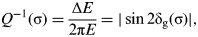 $$Q^{ - 1} ({\rm \sigma} ) = \displaystyle{{\Delta E} \over {2{\rm \pi} E}} = |\sin 2{\rm \delta} _{\rm g} ({\rm \sigma} )|,$$
where E is the total tidal energy stored in the planet, and ΔE is the energy dissipated per cycle. We can rewrite expression (12) as:
 $$b_{\rm g} ({\rm \sigma} ) = {\rm sign}({\rm \sigma} )\displaystyle{{k_2} \over {Q({\rm \sigma} )}}.$$
The present Q value for the planets in the Solar System can be estimated from orbital measurements, but as rheology of the planets is badly known, the exact dependence of b g(σ) on the tidal frequency σ is unknown. Many different authors have studied the problem and several models for b g(σ) have been developed so far, from the simplest ones to the more complex (for a review see Efroimsky & Williams Reference Efroimsky and Williams2009). The huge problem in validating one model better than the others is the difficulty to compare the theoretical results with the observations, as the effect of tides are very small and can only be detected efficiently after long periods of time. Therefore, here we only describe the most commonly models that are used (Fig. 2).
The visco-elastic model: In this model, Darwin (Reference Darwin1908) assumed that the planet behaves like a Maxwell solidFootnote 7 of constant density ρ, and found:
 $$b_{\rm g} ({\rm \sigma} ) = k_{\rm f} \displaystyle{{{\rm \tau} _{\rm b} - {\rm \tau} _{\rm a}} \over {1 + ({\rm \tau} _{\rm b} {\rm \sigma} )^2}} {\rm \sigma}, $$
where τa=υe/μe and τb are the time constants for damping of the body tides,
 $${\rm \tau} _{\rm b} = {\rm \tau} _{\rm a} (1 + 19{\rm \mu} _{\rm e} R/2Gm{\rm \rho} ).$$
The Maxwell solid model is usually accepted as a good approximation of the planet's response to tidal perturbations, although more complete visco-elastic models exist (for a review see Henning et al. Reference Henning, O'Connell and Sasselov2009). However, it depends on many uncertain parameters and it is not of practical use when we aim to do simple approximations and considerations on the tidal evolution. In addition, while it can be appropriate to simultaneously describe the elastic and viscous response of the solid body, it is questionable whether it is still valid for the atmospheric deformation is response to thermal gradients.
The viscous or linear model: in this model, it is assumed that the response time delay to the perturbation is independent of the tidal frequency, i.e., the position of the ‘maximal tide’ is shifted from the sub-stellar point by a constant time-lag Δt g (e.g, Mignard Reference Mignard1979). As usual we have σΔt g≪1, the viscous model becomes linear:
 $$b_{\rm g} ({\rm \sigma} ) = k_2 \sin \,({\rm \sigma} {\rm \Delta} t_{\rm g} ) \approx k_2 \,{\rm \sigma} {\rm \Delta} t_{\rm g}. $$
The viscous model is a particular case of the visco-elastic model and is specially adapted to describe the behaviour of planets in slow rotating regimes (ω~n).
The constant-Q model: for the Earth, Q changes by slightly more than an order of magnitude between the Chandler wobble period (about 440 days) and seismic periods of a few seconds (e.g., Anderson & Minster Reference Anderson and Minster1979; Karato & Spetzler Reference Karato and Spetzler1990). Thus, it is also common to treat the specific dissipation as independent of frequency:
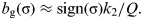 $$b_{\rm g} ({\rm \sigma} ) \approx {\rm sign}({\rm \sigma} )k_2 /Q.$$
The constant-Q model can be used for long periods of time where the tidal dissipation does not change much, as is the case for moderately rotating planets. However, for slow rotating planets, the constant-Q model is not appropriate as it gives rise to discontinuities for σ=0.
Core–mantle friction
We assume that the Earth-sized planets have internal structures similar to that of our planet, that is, these planets are composed of a solid mantle and a liquid core. We suppose that the liquid core is inviscid, incompressible and homogenous. We also suppose that the internal structure of the planets is unchanged in time, since the core formation time (or condensation velocity) is poorly known.
If there is slippage between the liquid core and the mantle, an additional source of dissipation of rotational energy results from friction occurring at the core–mantle boundary. Indeed, because of their different shapes and densities, the core and the mantle do not have the same dynamical ellipticity and the two parts tend to precess at different rates (Poincaré Reference Poincaré1910). This tendency is more or less counteracted by different interactions produced at their interface: the torque N of non-radial inertial pressure forces of the mantle over the core provoked by the non-spherical shape of the interface; the torque of the viscous (or turbulent) friction between the core and the mantle; and the torque of the electromagnetic friction, caused by the interaction between electrical currents of the core and the bottom of the magnetized mantle.
Poincaré's (Reference Poincaré1910) classic study shows that the core responds to the precession with a rotation velocity ωc, whose vector is inclined by a small angle χ with respect to the mantle velocity vector ω=ωk (Rochester Reference Rochester1976; Correia Reference Correia2006):
 $${\bf \delta} = {\bf \omega} - {\rm \omega} _{\rm c}, $$
and
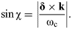 $$\sin {\rm \chi} = \left| {\displaystyle{{{\bf \delta} \times {\bf k}} \over {{\rm \omega} _{\rm c}}}} \right|.$$
Sasao et al. (Reference Sasao, Okubo and Saito1980) demonstrated that the pressure inertial torque may be expressed in a general way by:
 $${\bi N} = {\rm \omega} _{\rm c} \times {\bi L}_{\rm c} - {\bi P}_{\rm c}, $$
where Pc is the precession torque over the core and Lc its angular moment:
 $${\bi L}_{\rm c} = {{\bf \tilde { {\hskip2\cal I}}}}_{\rm c} \cdot {\bf \omega} _{\rm c}, $$
with
 $${{ \bf\tilde {{\hskip3 \cal I}}}}_{\rm c} = \left( {\matrix{ {A_{\rm c}} & 0 & 0 \cr 0 & {A_{\rm c}} & 0 \cr 0 & 0 & {C_{\rm c}} \cr}} \right).$$
C c and A c are the principal inertial moments of the core. The core's dynamical ellipticity is then given by E c=(C c−A c)/C c. The lower part of the mantle has irregularities that prevent the border between the two layers from being a perfect ellipsoid. According to Hide (Reference Hide1969) the height of these bumps may reach a few kilometres. Thus, for the dynamical ellipticity of the mantle, we establish that E c=E ch+δE c, that is, E c has a hydrostatic component and a non-hydrostatic component. For Earth, Herring et al. (Reference Herring, Gwinn and Shapiro1986) provide the value δE c=1.2×10⁻⁴.
The two types of friction torques (viscous and electromagnetic) depend on the differential rotation between the core and the mantle and can be expressed by a single effective friction torque, Φ. As a general expression for this torque, we adopt (Rochester Reference Rochester1976; Mathews & Guo Reference Mathews and Guo2005)
 $${\bf \Phi} = - ({\rm \kappa} + {\rm \kappa '}\,{\bf k} \times )\,{\bf \delta}, $$
where κ and κ′ are effective coupling parameters. Both parameters account for viscous and electromagnetic stresses at the core–mantle interface that can be written as: κ=κvis+κem and κ′=κ′vis+κ′em. Estimations for these coefficients can be found in the works of Mathews & Guo (Reference Mathews and Guo2005) and Deleplace & Cardin (Reference Deleplace and Cardin2006). In the simplified case of no magnetic field, the coupling parameters are only given by the viscous friction contributions, which can be simplified as (Noir et al. Reference Noir, Cardin, Jault and Masson2003; Mathews & Guo Reference Mathews and Guo2005):
 $${\rm \kappa} _{{\rm vis}} = 2.62\sqrt {{\rm \nu} |{\rm \omega} |} /R_{\rm c} \quad {\rm and}\quad {\rm \kappa '}_{{\rm vis}} = 0.259\sqrt {{\rm \nu} |{\rm \omega} |} /R_{\rm c}, $$
where R c is the core radius and ν the kinematic viscosity, which is poorly known. Even in the case of the Earth, the uncertainty in ν covers about 13 orders of magnitude (Lumb & Aldridge Reference Lumb and Aldridge1991), the best estimate so far being ν≃10−6 m2 s−1 (Gans Reference Gans1972; Poirier Reference Poirier1988; Wijs et al. Reference Wijs, Kresse and Vočadlo1998).
The contributions for spin variations of a planet may be obtained writing the equations of angular momentum conservation for the core and mantle:
 $$\displaystyle{{{\rm d}{\bi L}_{\rm m}} \over {{\rm d}t}} = {\bi P}_{\rm m} - {\bi N} - {\bf \Phi}, $$
 $$\displaystyle{{{\rm d}{\bi L}_{\rm c}} \over {{\rm d}t}} = {\bi P}_{\rm c} + {\bi N} + {\bf \Phi}, $$
where the Pm is the precession torque over the mantle and Lm is its angular momentum.
A general formulation for the equations of motion, valid for the both fast and slow rotation regimes of the planet, can be written as (Correia Reference Correia2006):
 $$\displaystyle{{{\rm d}L} \over {{\rm d}t}} \simeq - \displaystyle{{{\rm \kappa} A_{\rm c} C_{\rm c} {\rm \omega \alpha} ^2 \cos ^2 {\rm \varepsilon} \sin ^2 {\rm \varepsilon}} \over {(C_{\rm c} E_{\rm c} {\rm \omega} )^2 + {\rm \kappa} ^2}}, $$
 $$\hskip-98pt \displaystyle{{{\rm d}X} \over {{\rm d}t}} \simeq 0.$$
Dynamical analysis
Obliquity evolution
Until now, we have been expressing the variations of the spin in Andoyer's variables. Despite their practical use, these variables do not give a clear view of the obliquity variation. Since x=cos ε=X/L, one obtains:
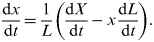 $$\displaystyle{{{\rm d}x} \over {{\rm d}t}} = \displaystyle{1 \over L}\left( {\displaystyle{{{\rm d}X} \over {{\rm d}t}} - x\displaystyle{{{\rm d}L} \over {{\rm d}t}}} \right).$$
For tidal effects (τ=g or τ=a), we express dx/dt using the eccentricity series for dL/dt and dX/dt (equations (10, 11) and (19, 20)):
 $$\eqalign{\displaystyle{{{\rm d}x} \over {{\rm d}t}} = & - \displaystyle{{K_{\rm \tau}} \over {\rm \omega}} \mathop \sum \limits_{\rm \sigma} b_{\rm \tau} ({\rm \sigma} )({\rm \Upsilon} _{\rm \sigma} - x{\rm \Lambda} _{\rm \sigma} ) \cr = & K_{\rm \tau} \displaystyle{{1 - x^2} \over {\rm \omega}} \mathop \sum \limits_{\rm \sigma} b_{\rm \tau} ({\rm \sigma} ){\rm \Theta} _{\rm \sigma} (x,e).} $$
We thus have
 $$\displaystyle{{{\rm d}x} \over {{\rm d}t}} \propto \displaystyle{{1 - x^2} \over {\rm \omega}} \displaystyle{{{\rm d}{\rm \omega}} \over {{\rm d}t}},$$
meaning that the obliquity variations are smaller than the rotation rate variations for initially fast rotating planets, and that  ${\rm \dot \varepsilon} \propto - \sin {\rm \varepsilon} $.
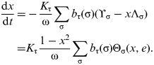
For the core–mantle friction effect, the variation of ε is easily computed from expression (39), since dX/dt≃0 (equation (38)).
 $$\displaystyle{{{\rm d}x} \over {{\rm d}t}} \simeq - \displaystyle{x \over L}\displaystyle{{{\rm d}L} \over {{\rm d}t}} = - \displaystyle{x \over {\rm \omega}} \displaystyle{{{\rm d}{\rm \omega}} \over {{\rm d}t}}$$
It also follows that
 $$X = cte.\quad \Rightarrow \quad x\,{\rm \omega} = cte.$$
Gravitational tides alone
From expression (18), we notice that for the initial stages of the evolution (σ≫n) atmospheric tides are weak. The same is true for core–mantle friction (equation (37)). As a consequence, gravitational tides dominate the spin evolution for fast rotating rates, thermal tides and core–mantle friction only playing a role for slow rotations (Correia et al. Reference Correia, Laskar and Néron de Surgy2003). Therefore, most studies on the spin evolution only consider gravitational tides. For a better comparison with our study, we recall here the main consequences of this effect alone.
If we assume a fast initial rotation, planets spend most of their evolution in the ω≫n regime. In this case, dω/dt evolves independently of the dissipative model, because all the terms in expression (10) have the same sign. Thus, in this regime gravitational tides always decrease the rotation rate, since K g<0 (equation (9)).
When the planet arrives in the slow rotation regime (ω~n), some of the terms in equation (10) become negative and we can no longer generalize our conclusions to all dissipative models. However, in the vicinity of tidal frequencies near zero (σ≈0), except for the constant – Q model, all dissipative models can be made linear (Fig. 2). Then, adopting the linear dissipation model described in the ‘Tidal models’ subsection, we can write
 $$b_{\rm g} ({\rm \sigma} ) \simeq k_2 {\rm \sigma} {\rm \Delta} t_{\rm g} = \displaystyle{{k_2} \over {Q_n}} \displaystyle{{\rm \sigma} \over {2n}},$$
where Q n−1=2nΔt g is the specific dissipation factor for small frequencies. For small eccentricity, the highest tidal frequency is σ=2ω+3n (equation (19)), so this approximation is validFootnote 8 for Q n≳5.
In the limit of slow rotation rates, we can then simplify expression (10):
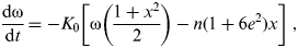 $$\displaystyle{{{\rm d}{\rm \omega}} \over {{\rm d}t}} = - K_0 \left[ {{\rm \omega} \left( {\displaystyle{{1 + x^2} \over 2}} \right) - n(1 + 6e^2 )x} \right]\;, $$
where
 $$K_0 = - \displaystyle{{3K_{\rm g} k_2 \Delta t_{\rm g}} \over C}\left( {1 + \displaystyle{{15} \over 2}e^2} \right)\;. $$
Thus, for each obliquity there is an equilibrium value for the rotation rate ωe, obtained when dω/dt=0:
 $$\displaystyle{{{\rm \omega} _{\rm e}} \over n} = (1 + 6e^2 )\displaystyle{{2x} \over {1 + x^2}}. $$
For ω>ωe the rotation rate decreases, whereas for ω<ωe it increases.
Equilibrium damping time
In order to check if the spin of a given planet is still evolving or if it can be found at its equilibrium rotation, we can compute an evolutionary characteristic time and then compare it to the age of the host star. Since gravitational tides are the dominant effect for the most part of the evolution, we can use this effect alone to estimate the characteristic time τeq needed to reach the equilibrium rotation. Thus, from expression (45) we get:
 $${\rm \tau} _{{\rm eq}} \sim \displaystyle{1 \over {K_0}} = \displaystyle{{GC} \over {3k_2 \Delta t_{\rm g} R^5}} \displaystyle{1 \over {n^4}} = \displaystyle{{ma^6} \over {9GM_*^2 k_2 \Delta t_{\rm g} R^3}}, $$
with C≈m R 2/3 and n 4=G 2M *2/a 6. In Table 1, we computed the characteristic times for existing Earth-sized exoplanets. We notice that, except for GJ 667C g, all known planets have a τeq lower than the age of the system, and so it is believed that they have already reached an equilibrium rotation state.
Table 1. Characteristics and equilibrium rotation rates of Earth-sized planets with masses lower than 10 M ⊕ (see text for notations)
a Using Equation (48) with k 2=1/3 and Δt g=640 s (Earth's values). References: 1) Rappaport et al. (Reference Rappaport, Sanchis-Ojeda, Rogers, Levine and Winn2013b); 2) Charpinet et al. (Reference Charpinet2011); 3) Rappaport et al. (Reference Rappaport, Barclay and DeVore2013a); 4) Muirhead et al. (Reference Muirhead, Johnson and Apps2012); 5) Callegari & Rodríguez (Reference Callegari and Rodríguez2013); 6) Dumusque et al. (Reference Dumusque, Pepe and Lovis2012); 7) Xie (Reference Xie2013); 8) Hadden & Lithwick (Reference Hadden and Lithwick2013); 9) Chaplin et al. (Reference Chaplin, Sanchis-Ojeda and Campante2013); 10) Sanchis-Ojeda et al. (Reference Sanchis-Ojeda, Rappaport and Winn2013); 11) Pepe et al. (Reference Pepe, Cameron and Latham2013); 12) Lopez & Fortney (Reference Lopez and Fortney2013); 13) Lissauer et al. (Reference Lissauer, Fabrycky and Ford2011); 14) Forveille et al. (Reference Forveille, Bonfils and Delfosse2011); 15) Pepe et al. (Reference Pepe, Lovis and Ségransan2011); 16) Anglada-Escudé et al. (Reference Anglada-Escudé, Tuomi and Gerlach2013); 17) Fressin et al. (Reference Fressin, Torres and Rowe2012); 18) Tuomi et al. (Reference Tuomi, Anglada-Escudé and Gerlach2013); 19) Borucki et al. (Reference Borucki, Agol and Fressin2013); 20) Jontof-Hutter et al. (Reference Jontof-Hutter, Lissauer, Rowe and Fabrycky2013); 21) Howard et al. (Reference Howard, Johnson and Marcy2011); 22) Carter et al. (Reference Carter, Agol and Chaplin2012); 23) Anglada-Escudé & Tuomi (Reference Anglada-Escudé and Tuomi2012); 24) Batalha et al. (Reference Batalha, Borucki and Bryson2011); 25) Gilliland et al. (Reference Gilliland2013); 26) Vogt et al. (Reference Vogt, Wittenmyer and Butler2010) 27) Steffen et al. (Reference Steffen, Fabrycky and Agol2013); 28) Delfosse et al. (Reference Delfosse, Bonfils and Forveille2013); 29) Rivera et al. (Reference Rivera, Butler and Vogt2010a); 30) Harpsøe et al. (Reference Harpsøe, Hardis and Hinse2013); 31) Ofir et al. (Reference Ofir, Dreizler, Zechmeister and Husser2013); 32) Lo Curto et al. (Reference Lo Curto, Mayor and Benz2010); 33) Rivera et al. (Reference Rivera, Laughlin and Butler2010b); 34) Cochran et al. (Reference Cochran2011); 35) Bonfils et al. (Reference Bonfils, Gillon and Forveille2011); 36) Holman et al. (Reference Holman, Fabrycky and Ragozzine2010); 37) Torres et al. (Reference Torres, Fressin and Batalha2011); 38) Léger et al. (Reference Léger, Rouan and Schneider2009); 39) Bouchy et al. (Reference Bouchy, Mayor and Lovis2009); 40) Henry et al. (Reference Henry, Howard, Marcy, Fischer and Johnson2011); 41) Endl et al. (Reference Endl, Robertson and Cochran2012); 42) Queloz et al. (Reference Queloz, Bouchy and Moutou2009); 43) Forveille et al. (Reference Forveille, Bonfils and Delfosse2009); 44) Lo Curto et al. (Reference Lo Curto, Mayor and Benz2013); 45) Gautier et al. (Reference Gautier, Charbonneau and Rowe2012); 46) Jenkins et al. (Reference Jenkins, Tuomi, Brasser, Ivanyuk and Murgas2013); 47) Howard et al. (Reference Howard, Johnson and Marcy2009); 48) Lovis et al. (Reference Lovis, Mayor and Pepe2006); 49) Howell et al. (Reference Howell, Rowe and Bryson2012); 50) Weiss & Marcy (Reference Weiss and Marcy2013); 51) Pepe et al. (Reference Pepe, Correia and Mayor2007).
Thermal tides effect
We now include in our analysis the effect from thermal atmospheric tides to the spin evolution (subsection ‘Thermal atmospheric tides’). As shown earlier, the averaged variation of the spin can be expressed by equation (10) for gravitational tides and by equation (19) for atmospheric tides. Considering that the planet's obliquity is small (ε~0), we can neglect terms of order ε2 or higher in equations (10) and (19). In this case, the variation of the spin caused by gravitational tides is then (Correia et al. Reference Correia, Levrard and Laskar2008):
 $$\eqalign{ T_{\rm g} =\ &\left. {\displaystyle{{{\rm d}L} \over {{\rm d}t}}} \right]_{\rm g} = \displaystyle{3 \over 2}K_{\rm g} \left[ {(1 - 5e^2 )b_{\rm g} (2{\rm \omega} - 2n)} \right. \cr & \left. { + \displaystyle{1 \over 4}e^2 b_{\rm g} (2{\rm \omega} - n) + \displaystyle{{49} \over 4}e^2 b_{\rm g}\right. \left. (2{\rm \omega} - 3n)} \big].} $$
In the same way, for thermal atmospheric tides we obtain
 $$\eqalign{ T_{\rm a} =\ &\left. {\displaystyle{{{\rm d}L} \over {{\rm d}t}}} \right]_{\rm a} = \displaystyle{3 \over 2}K_{\rm a} \left[ {(1 - 3e^2 )b_{\rm a} (2{\rm \omega} - 2n)} \right. \cr & \left. { - e^2 b_{\rm a} (2{\rm \omega} - n) + 9e^2 b_{\rm a} (2{\rm \omega} - 3n)} \right]\;.} $$
As the time-lag from gravitational and atmospheric tides is poorly known, in this section we use again the viscous model. Since σΔt is usually small, then:
 $$b_{\rm g} ({\rm \sigma} ) \simeq k_2 {\rm \sigma} {\rm \Delta} t_{\rm g} \quad {\rm and}\quad b_{\rm a} ({\rm \sigma} ) \simeq - |\tilde p_2 |{\rm \sigma} {\rm \Delta} t_{\rm a}. $$
 For atmospheric tides it is also necessary to consider the response of the surface pressure variations to tidal frequency (equation (18)). We use the ‘heating at the ground’ model, described by Dobrovolskis & Ingersoll (Reference Dobrovolskis and Ingersoll1980). It is supposed that all the stellar flux absorbed by the ground, F s, is immediately deposited in a thin layer of atmosphere at the surface. The heating distribution is then written as a delta-function just above the ground ( $J_{\rm \sigma} = gF_{\rm s} /\tilde p_0 $). Besides the good agreement with the observations, this approximation is justified because tides in the upper atmosphere are decoupled from the ground by the disparity between their rotation rates. Neglecting υσ over the thin heated layer, equation (18) becomes:
 $${\rm {\cal P}}_{\rm \sigma} = F_{\rm s} /(8H_0 ) \propto L_* /a^2, $$
where L * is the star luminosity and a the semi-major axis.
The average evolution of the rotation rate can then be obtained adding the effects of both tidal torques acting on the planet:
 $$\displaystyle{{{\rm d}L} \over {{\rm d}t}} = C{\rm \dot \omega} = (T_{\rm g} + T_{\rm a} ).$$
Substituting in previous expression T g and T a given by equations (49) and (50) together with the viscous dissipative model (equation (51)), we haveFootnote 9:
 $$\eqalign{ \displaystyle{{{\rm \dot \omega}} \over { - K_0}} =\ & {\rm \omega} - (1 + 6e^2 )n - {\rm \omega} _{\rm s} \left[ {\left( {1 - \displaystyle{{21} \over 2}e^2} \right){\rm sign}({\rm \omega} - n)} \right. \cr & \left. { - e^2 {\rm sign}(2{\rm \omega} - n) + 9e^2 {\rm sign}(2{\rm \omega} - 3n)} \bigg]} $$
with
 $${\rm \omega} _{\rm s} = \displaystyle{{K_{\rm a} F_{\rm s} \Delta t_{\rm a}} \over {16H_0 K_{\rm g} k_2 \Delta t_{\rm g}}} \propto \displaystyle{{L_* R} \over {M_* m}}a.$$
Equilibrium final states for the rotation rate
An equilibrium final state occurs when  ${\rm \dot \omega} = 0$. From equation (53) this happens when T g=−T a. When e=0 (see Correia & Laskar Reference Correia and Laskar2001),
 $$f\,({\rm \omega} - n) = - \displaystyle{{T_{\rm g}} \over {T_{\rm a}}} = - \displaystyle{{K_{\rm g} b_{\rm g} (2{\rm \omega} - 2n)} \over {K_{\rm a} b_{\rm a} (2{\rm \omega} - 2n)}} = 1\;, $$
where f(x) is an even function of x. For the dissipative model in use, we can assume that f(x) is monotonic close to equilibrium, and so we haveFootnote 10:
 $$|{\rm \omega} - n| = f^{ - 1} (1) = {\rm \omega} _{\rm s}. $$
This means that there are two final possibilities for the equilibrium rotation of the planet:
 $${\rm \omega} ^ \pm = n \pm {\rm \omega} _{\rm s}. $$
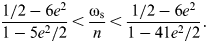
If ωs<n, all final states correspond to prograde final rotation rates (Fig. 3(a) and (b)). Retrograde rotation appears only if the planet evolves to the ω− state together with ωs>n. As we can see in Table 1, this is the case of planet Venus (Fig. 3(c)).
Fig. 3. Variation of  ${\rm \dot \omega} $ with ω/n (equation (54)) for (a) ωs/n=0.05, (b) ωs/n=0.55 and (c) ωs/n=1.92, using different eccentricities (e=0.0, 0.1, 0.2). The equilibrium rotation rates are given by ${\rm \dot \omega} $=0 and the arrows indicate whether it is a stable or unstable equilibrium position.
For moderate values of the eccentricity and using equations (49) and (50), equation (56) can be rewritten as:
 $$f\,({\rm \omega} - n) = 1 - e^2 \left( {2 + \displaystyle{{g({\rm \omega} )} \over {b_{\rm a} (2{\rm \omega} - 2n)}}} \right),$$
where
 $$\eqalign{g({\rm \omega} ) = & \displaystyle{{K_{\rm g}} \over {4K_{\rm a}}} [b_{\rm g} (2{\rm \omega} - n) + 49b_{\rm g} (2{\rm \omega} - 3n)] \cr & - b_{\rm a} (2{\rm \omega} - n) + 9b_{\rm a} (2{\rm \omega} - 3n).} $$
When we compute the inverse function of previous equation and use ωs from expression (57) we get:
 $$|{\rm \omega} - n| = f^{ - 1} (1) - e^2 \left( {2 + \displaystyle{{g({\rm \omega} )} \over {b_{\rm a} (2{\rm \omega} - 2n)}}} \right)\left. {\displaystyle{{\partial f^{ - 1}} \over {\partial x}}} \right|_{x = 1}, $$
which means that we now have four final possibilities for the equilibrium rotation of the planet:
 $${\rm \omega} _{1,2}^ \pm = n \pm {\rm \omega} _{\rm s} + e^2 {\rm \delta} _{1,2}^ \pm, $$
with
 $${\rm \delta} _{1,2}^ \pm = \left( {2 + \displaystyle{{g({\rm \omega} )} \over {|b_{\rm a} (2{\rm \omega} - 2n)|}}} \right)\left. {\displaystyle{{\partial f^{ - 1}} \over {\partial x}}} \right|_{x = 1} \;. $$
Adopting the dissipation model from equation (51) and using expression (54), we find that ω2+ occurs when ω>3n/2 and
 $$\eqalign{{\rm \omega} _2^ + =\ & (1 + 6e^2 )n + {\rm \omega} _{\rm s} \left[ {1 + e^2 \left( {9 - \displaystyle{{21} \over 2} - 1} \right)} \right] \cr =\ & n + {\rm \omega} _{\rm s} + e^2 \left( {6n - \displaystyle{5 \over 2}{\rm \omega} _{\rm s}} \right).} $$
Similarly, we find the ω1+ state when n<ω<3n/2
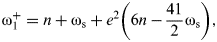 $${\rm \omega} _1^ + = n + {\rm \omega} _{\rm s} + e^2 \left( {6n - \displaystyle{{41} \over 2}{\rm \omega} _{\rm s}} \right),$$
when n/2<ω<n we have the ω1− state
 $${\rm \omega} _1^ - = n - {\rm \omega} _{\rm s} + e^2 \left( {6n + \displaystyle{1 \over 2}{\rm \omega} _{\rm s}} \right),$$
and finally for ω<n/2 we have
 $${\rm \omega} _2^ - = n - {\rm \omega} _{\rm s} + e^2 \left( {6n + \displaystyle{5 \over 2}{\rm \omega} _{\rm s}} \right).$$
Then, expression (63) can be rewritten as:
 $${\rm \delta} _{1,2}^ - = 6n + \left( {\displaystyle{3 \over 2} \pm 1} \right){\rm \omega} _{\rm s} $$
and
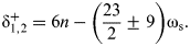 $${\rm \delta} _{1,2}^ + = 6n - \left( {\displaystyle{{23} \over 2} \pm 9} \right){\rm \omega} _{\rm s}. $$
As the set of final states ω1,2± must also verify
 $${\rm \omega} _2^ - \lt n/2 \lt {\rm \omega} _1^ - \lt n \lt {\rm \omega} _1^ + \lt 3n/2 \lt {\rm \omega} _2^ +, $$
in general, and depending on the values of ωs and e, these four equilibrium rotation states cannot coexist all simultaneously. In particular, when we adopt the viscous tidal model (equation (51)), the final states ω1− and ω1+ never coexist with ω2−. At most three different equilibrium states are therefore possible, obtained when ωs/n is close to 1/2, or more precisely, when
 $$\displaystyle{{1/2 - 6e^2} \over {1 - 5e^2 /2}} \lt \displaystyle{{{\rm \omega} _{\rm s}} \over n} \lt \displaystyle{{1/2 - 6e^2} \over {1 - 41e^2 /2}}.$$
Conversely, we have that ω1+ is the single final state that exists whenever ωs/n<6e 2(1+e 2/2).
In Fig. 3, we plot some examples for the rotation rate evolution for some ωs and eccentricity values. We see that when ωs/n is close to zero only the final equilibrium state ω1+ is possible (Fig. 3(a)). For ωs/n=1.92, the Venus value, two final equilibrium states are possible: the ω2− and the ω2+ (Fig. 3(c)). However, when ωs/n=0.55 we still have two possible states for e=0.0 (ω1− and ω1+), but there are three possible final states for e>0.1 (ω1−,ω1+ and ω2+) (Fig. 3(b)).
In Fig. 4, we plot the possible equilibrium rotation states as a function of ωs/n for eccentricities of e=0.0, 0.1 and 0.2. Depending on ωs/n and the eccentricity values, the planet may have one, two or three possibilities to evolve. If ωs/n is close to 0.5 the planet has more possible final states (equation (71)): if the eccentricity is zero, the planet has two possible final states, but if the eccentricity of the planet is 0.1 or 0.2 there are three possibilities. We can also note that for e=0, retrogade states appear when ωs/n⩾1, but for e=0.1 and e=0.2 the rotation rate must be slightly higher. More exactly, it is needed that ωs/n⩾(1+17e 2/2), i.e., ωs/n⩾1.09 for e=0.1, and ωs/n⩾1.34 for e=0.2.
Fig. 4. Equilibrium positions of the rotation rate as a function of the ratio ωs/n for three different values of the eccentricity: (a) e=0.0, (b) e=0.1 and (c) e=0.2. The solid red line corresponds to the ω1+ state, the dotted red to the ω1− state, the solid blue line to the ω2+ state, and the dotted blue line to the ω2− state.
Application to already known exoplanets
Although we have witnessed in the last few years an increase in the discovery of Earth-sized exoplanets, the physical data for these planets are still scarce. Hence, we can only do some assumptions that allow us to infer some constraints on their final spin evolution. We assume here that these planets are rocky with a dense atmosphere like Venus (Alibert et al. Reference Alibert, Baraffe and Benz2006; Rafikov Reference Rafikov2006). We can call these Earth-sized exoplanets as V-type planets. Using the empirical mass–luminosity relation L *∝M *4 (Cester et al. Reference Cester, Ferluga and Boehm1983) and the mass–radius relation for terrestrial planetsFootnote 11R ∝ m 0.274 (Sotin et al. Reference Sotin, Grasset and Mocquet2007), we get from equation (55):
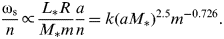 $$\displaystyle{{{\rm \omega} _{\rm s}} \over n} \propto \displaystyle{{L_* R} \over {M_* m}}\displaystyle{a \over n} = k(aM_* )^{2.5} m^{ - 0.726}. $$
k is a coefficient of proportionality containing the parameters that we cannot constrain for these planets (H 0, F s, k 2, Δt g and Δt a). Assuming that all unknown properties of the Earth-sized planets are the same as for Venus (2π/ωs=116.1 day, and so ωs/n=1.9255), we computeFootnote 12:
 $$k = \displaystyle{{{\rm \omega} _{\rm s}} \over n}(aM_* )^{ - 2.5} m^{0.726} = 3.73({\rm AU}\;M_ \odot )^{ - 2.5} \,m_ \oplus ^{0.726} $$
Using the previous equation, we can estimate the ωs/n ratio for all known Earth-sized planets (Table 1).
As shown in equation (72), ωs/n is a function of the product aM *. To see how the equilibrium rotation rate states depend on these parameters, in Fig. 5 we plot the number of values of the equilibrium rotation states as a function of aM *, for eccentricities e=0.0, 0.1 and 0.2. We can compare Fig. 5 with Table 1, where the planet's parameters and the possible final equilibrium states are presented. The actual rotation state of the planet Venus corresponds to the ω2− equilibrium state. For the remaining exoplanets here studied, only one equilibrium rotation state is possible, the ω1+ state. There is only one exception, planet HD 40307 f, which has two possible equilibrium states (ω1+ and ω1−), but their values are too close to be distinguished in a future direct observation of the planet.
Fig. 5. Equilibrium positions of the rotation rate as a function of the product aM * for three different values of the eccentricity: (a) e=0.0, (b) e=0.1 and (c) e=0.2. The solid red line corresponds to the ω1+ state, the dotted red line to the ω1− state, the solid blue line to the ω2+ state, and the dotted blue line to the ω2− state.
The aM * value for all planets listed in Table 1 is small as a consequence of the present limitations of the detection techniques: at present we are only able to detect Earth-sized planets orbiting very close to low-mass stars, for which gravitational tides dominate.
Generalization to Earth-sized planets
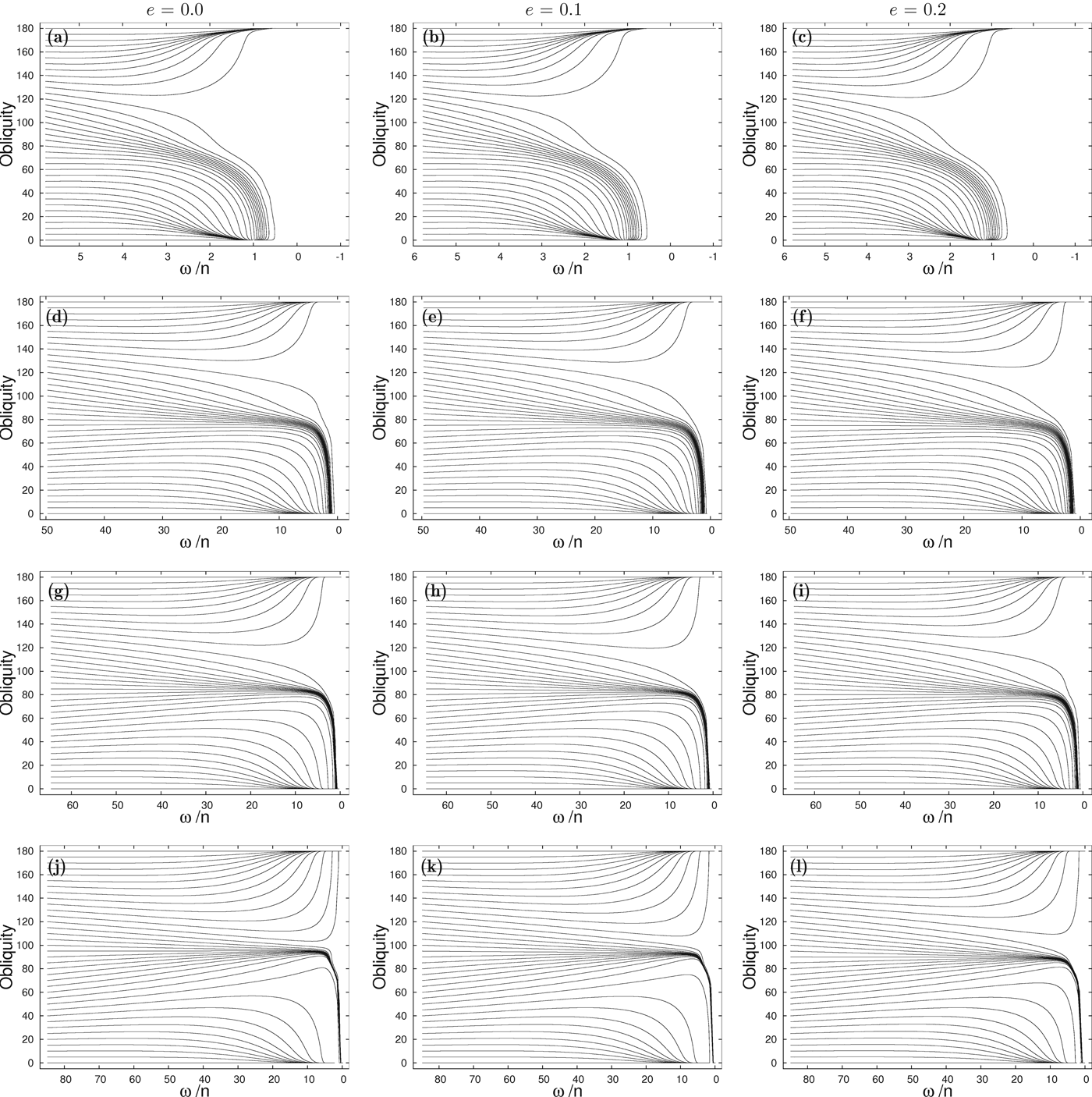
With the continuous increase in the precision of detection methods, we expect to soon find planets orbiting Sun-like stars as distant from them as the Earth or Venus are from the Sun (e.g., D'Odorico & CODEX/ESPRESSO Team Reference D'Odorico2007). Foreseeing this situation, we applied the previous calculations to long-period Earth-sized planets that may eventually be found in the HZ of these systems.
Assuming that the planet's mass and radius are the same of Venus and a host star with the mass of the Sun, we made calculations for three different values of the eccentricity (e=0.0, 0.1 and 0.2), varying for each one the value of the semi-major axis a. As expected, more possible equilibrium rotation states appear (Table 2). For the same eccentricity we note that the difference in the rotation period of the several equilibrium states is enlarged by the distance to the star. We can also see that for higher values of aM * retrograde states may be possible. Setting ω2−<0 (equation (67)) and substituting ωs/n by equation (72), we may find the value of rotation rate needed for a retrograde state:
 $$aM_* \geqslant \left[ {\displaystyle{1 \over {3.73}}\left( {1 + \displaystyle{{17} \over 2}e^2} \right)} \right]^{0.4}. $$
Table 2. Characteristics and equilibrium rotation rates of Venus-like planets orbiting a Sun-like star (M*=M⊙)
Thus, for zero eccentricity a retrograde state is possible when aM *≳0.59, for e=0.1 a possible retrograde states appears when aM *≳0.61, whereas for an eccentricity of e=0.2, we need aM *≳0.66 for retrograde rotation. This is also confirmed in Fig. 5, where we can see that planets with eccentricities of e=0.1 and 0.2 have a retrograde equilibrium state for an aM * product higher than 0.6. Table 2 and Fig. 5 are also in agreement on the number of states when aM * is around 0.45 AU M ⊙. Although only two states can be found when the eccentricity is zero, for eccentricities of 0.1 and 0.2 we find three equilibrium states.
Numerical simulations
An interpolated dissipative model
During the spin evolution of the planets, the tidal frequency varies and so does the dissipation factors b(σ) (equations (12) and (17)). Because the rheology of the planets is poorly known, the exact dependence of the dissipation on the tidal frequency is unknown. In the ‘Tidal models’ subsection, we described the most commonly used dissipation models (Fig. 2). However, the visco-elastic model seems inappropriate for atmospheric tides, whereas the viscous one is not realistic for σ≫n, and the constant – Q for σ=n. More complex models exist (e.g., Efroimsky & Williams Reference Efroimsky and Williams2009), but for simplicity we adopt here an interpolated model that behaves like the linear model for small values of σ and like the constant – Q model when σ increases (e.g., Ćuk & Stewart Reference Ćuk and Stewart2012). This model is also in agreement with the analytical simplifications from the ‘Dynamical analysis’ section. It is also very close to the models obtained by Remus et al. (Reference Remus, Mathis and Zahn2012) in their construction of a tidal model for small and moderate spin rates based on hydrodynamical equations (see Fig. 4 in Remus et al. Reference Remus, Mathis and Zahn2012).
For gravitational tides the time-lag is then given by
 $$b_{\rm g} ({\rm \sigma} ) = k_2 {\rm \sigma} {\rm \Delta} t_{\rm g} ({\rm \sigma} ) = \displaystyle{{k_2} \over {2Q_n}} \left[ {\displaystyle{{\rm \sigma} \over n} + \left( {2\,{\rm sign}({\rm \sigma} ) - \displaystyle{{\rm \sigma} \over n}} \right){\rm \xi} ({\rm \sigma} )} \right]\;, $$
where ξ(σ) is a function varying between 0 and 1, used to make a smooth passage between the two regimes:
 $${\rm \xi} ({\rm \sigma} ) = \displaystyle{1 \over 2} + \displaystyle{1 \over 2}\tanh {\rm \;} \left( {\displaystyle{{|{\rm \sigma} |} \over n} - 2} \right).$$
In Fig. 6, we plot the above expressions as a function of the tidal frequency. The transition of regime occurs for σc=2n, and Q n corresponds to the dissipation Q – factor during the constant phase.
Fig. 6. (a) ξ(σ) versus σ with σc/n=2; (b) behaviour of b g(σ) using the interpolated model smoothed by ξ(σ).
For thermal atmospheric tidesFootnote 13, the time-lag Δt a(σ) is simply obtained from expression (55):
 $${\rm \Delta} t_{\rm a} ({\rm \sigma} ) = {\rm \Delta} t_{\rm g} ({\rm \sigma} )\displaystyle{{16H_0 K_{\rm g} k_2} \over {K_{\rm a} F_{\rm s}}} {\rm \omega} _{\rm s}. $$
Choice of parameters
Since much is unknown about exoplanets, we need to make some assumptions in our simulations. As we already stated, we consider here V-type planets. We assume that these planets with masses lower than 10 M ⊕ have a structure similar to the terrestrial planets of the Solar System, and a dense atmosphere capable of influencing their spin evolution. Thus, for a given exoplanet, we adopt for the unknown parameters the corresponding value from VenusFootnote 14. Therefore, in our simulations we take the potential Love number k 2=0.28, Q n=50, the mean density,  $\bar {{ \rm \rho}} = 5.24 \times 10^3 \;{\rm kg}\;{\rm m} ^{- 3} $, and the stellar energy that reaches the planet surface F s=100 W m−2. For the mantle dynamic ellipticity we adopt δE d=1.3×10⁻⁵ and for the kinematic viscosity ν=10−6 m2 s−1. For the core radius R c=3.1×10⁶ m, the planet structure coefficient C/mR 2=0.336, and the ratio between the core moment of inertia and moment of inertia C c/C=0.084 (Yoder Reference Yoder1995, Reference Yoder1997).
In our simulations we start with P in=1 or 2 days, a rotation period that is faster than the predicted present rotation. Since some of these planets orbit very close to the star, and hence end up with fast equilibrium rotations (e.g., planet 55 Cnc e, whose final rotation is estimated to be 0.733 day), we also tested the possibility of planets evolved from a slower rotation to a faster one, with P in=25 days. The results of these simulations are presented in the next two sections.
Application to already known exoplanets
In Fig. 7, we show the spin evolution for the planets HD 40307 b and g with time. We adopted P in=1 day and initial obliquities ranging from 0° to 180°, with a step of 5°. Although the initial rotation rate is the same for planets b and g, the initial ratio ω/n is much higher for planet g, because the mean motion n is smaller. As a consequence, the characteristic evolution timescale is about 100 yr for planet b, while it is 1 Gyr for planet g. Those values are in agreement with the ones computed using equation (48) (Table 1). After that time all trajectories reach a final equilibrium for the spin, but depending on the initial value of the obliquity, the exact time can be different. Contrary to what we could expect, initial obliquities close to 180°, usually take less time to reach the equilibrium than lower initial values. This can be understood, since for high obliquities there are more harmonics with significant value that contribute to the spin evolution (equations (10, 11)).
Fig. 7. Spin evolution with time for the planets HD 40307 b (left) and HD 40307 g (right), with P in=1 day and initial obliquities ranging from ε=0° to 180°. We plot the obliquity (top) and ω/n (bottom) evolution. Each line represents a different initial obliquity value. The lower lines in the ω/n plot correspond to the initial obliquities closer to 180°.
At first glance it may seem that there are two final equilibrium rotation states: one for final obliquities equal to 0°, and another for 180°. However, all initial obliquities evolve into the 2π/ω1+ final rotation state, the only possibility for these two planets (Table 1). For the initial obliquities close 0°, the rotation rate is always positive and the obliquity is decreased to zero degrees. For initial obliquities close 180° the obliquity evolves into this value, while the rotation rate slows down until zero and then increases in the other way, until it stabilizes at a negative value −2π/|ω1+|. This is the same as having a planet with zero obliquity rotating prograde, that is, the couple (−ω, π−ε) is mathematically equivalent to (ω, ε). Therefore, there are two different paths, but they lead to the same final equilibrium. This has also been described for Venus (Correia & Laskar Reference Correia and Laskar2001, Reference Correia and Laskar2003b).
It is also interesting to note that for initial obliquities around 90°, the rotation rate decreases to a value lower than that of equilibrium, and then it increases again until equilibrium is reached. This behaviour is in agreement with expression (47).
Comparing the rotation rate and the obliquity evolutions shown in Fig. 7 we also note that the obliquity is initially slightly constant and takes more time to reach the equilibrium than the rotation rate. The explanation for this behaviour is given in the ‘Obliquity evolution’ subsection. As we can see from expression (41), the obliquity variation is inversely proportional to the rotation rate. Thus, for a fast initial rotation, the obliquity does not change much. This is particularly visible for HD 40307 g, since the initial rotation ω≫n. However, as the rotation rate decreases we observe a strong variation in the obliquity. Finally, the obliquity slowly decreases into zero, since dx/dt∝(1−x 2)⇔dε/dt∝−sinε (equation (40)).
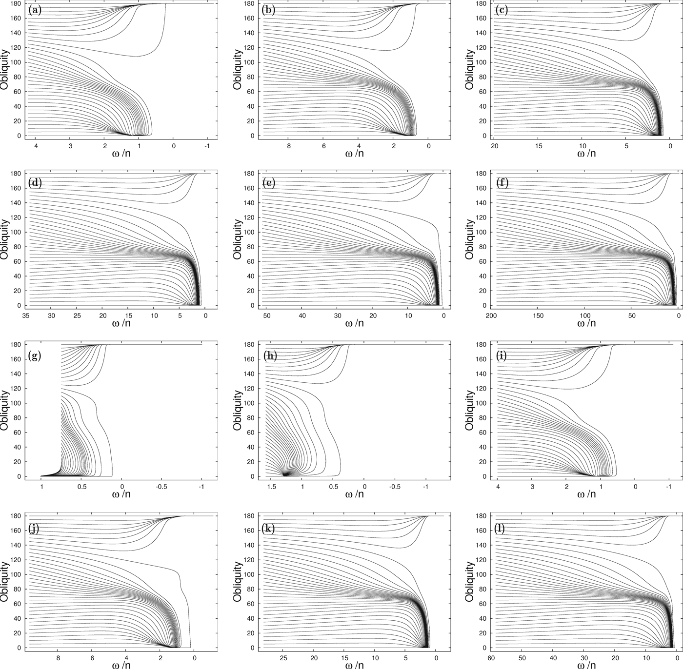
In Fig. 8, we show the obliquity evolution with the rotation rate ω/n for many systems listed in Table 1 (including HD 40307 b and g), always starting with an initial rotational period P=1 day. We observe again the dichotomy in the obliquity evolution: it can only end up in 0° or 180°. This result was demonstrated in Correia et al. (Reference Correia, Laskar and Néron de Surgy2003) for Venus’ parameters, but it seems to remain valid for all Earth-sized planets, even for those in eccentric orbits. This is in agreement with the assumption ε≃0° that we made when looking for final states (subsection ‘Equilibrium final states for the rotation rate’).
Fig. 8. Obliquity evolution with the rotation rate for several Earth-sized planets taken from Table 1 with an initial rotation period of P in=1 day: (a) to (f) HD 40307 b to g; (g) 55 Cnc e; (h) GJ 1214 b; (i) HD 215497 b; (j) μ Arae c; (k) GJ 667C c; (l) HD 85512 b.
As a result of the obliquity's dichotomy, it appears that all planets have two possible final states, one prograde and another retrograde. For most of them only one final rotation state is possible, we are just observing the equivalent couples (ω, ε) and (−ω, π−ε). However, in one case for HD 40307 f (Fig. 8(e)), we can indeed observe two final rotation possibilities, the states ω1+ and ω1− (Table 1). As these two states are so close to each other, it is nonetheless very difficult to distinguish them in the figure.
For all planets shown in Fig. 8, we also observe that the obliquity evolves into its final position at 0° or 180° always before ω/n=0. The reason is that for very slow rotation rates, core–mantle friction becomes dominating over tidal effects (equation (42)), quickly driving the obliquity to its final position. Therefore, the transition from positive into negative rotation rates only occurs at obliquities very close to 0° or 180°.
In the case of 55 Cnc e (Fig. 8(g)), we initially have ω/n≈0.76, that is, the initial rotation period of the planet is slower than the orbital period. As a consequence, contrarily to the remaining examples in Fig. 8, the rotation rate needs to increase its value to reach the equilibrium value near the synchronous rotation. We indeed observe this behaviour for initial obliquities close to 0°. However, for initial obliquities higher than 30°, the rotation rate still decreases to a lower ratio ω/n<0.76, before evolving into to the final equilibrium rotation. The explanation for this behaviour can be found in equation (47): for non-zero obliquities, the equilibrium rotation rate is below the synchronous rotation, so as long as the obliquity remains high we have 0<ω/n<1.
In Fig. 9, we show again the obliquity evolution with the rotation rate ω/n for the same systems in Fig. 8, but now starting with a slower rotation period P in=25 days. Since most planets discovered so far are close-in planets with orbital periods smaller than 25 days, we now have an initial rotation rates ω<n for these planets. As a consequence, we observe an identical behaviour as the one described for 55 Cnc e with P in=1 day (Fig. 8(g)).
Fig. 9. Obliquity evolution with the rotation rate for several Earth-sized planets taken from Table 1 with an initial rotation period of P in=25 days: (a) to (f) HD 40307 b to g; (g) 55 Cnc e; (h) GJ 1214 b; (i) HD 215497 b; (j) μArae c; (k) GJ 667C c; (l) HD 85512 b.
Although the spin evolution with ω<n (Fig. 9) is completely different from the situation with ω>n (Fig. 8), the final rotation states are exactly the same. Different initial conditions lead to alternative evolutionary paths, but the final picture is the same. However, when ω<n we observe that there are much more trajectories increasing its obliquity to 180°. This behaviour is related to the onset of core–mantle friction. From equation (43) we have that (1) this effect is stronger for slow rotation rates; (2) when this effect becomes dominating, the obliquity evolves into 180° if ε>90° (x f=x 0ω0/ωf). Indeed, in Fig. 9 we clearly observe that when ω/n~0 there is a sudden inversion of the obliquity trend, whose final evolution is dictated by the 90° threshold.
We conclude that gravitational tides control the initial stages of the evolution, and that thermal atmospheric tides are only important in the definition of the final equilibrium rotation. Core–mantle friction only becomes important in the slow rotation regime (ω~n), but for very slow rotations it rules over both tidal effects.
Earth-sized planets in the habitable zone
Since most existing terrestrial planets are very close to their parent stars and/or orbit low-mass stars, usually there is only one final equilibrium rotation rate, given by state ω1+ (Fig. 5, Table 1). In the examples from Figs. 8 and 9, only for HD 40703 f two final states are possible, but yet they are very close to each other and hardly distinguishable. As a consequence, in the simulations from the previous section, we were unable to observe evolutionary paths leading to very different configurations, such as retrograde rotation.
In the ‘Generalization to Earth-sized planets’ subsection, we investigated the most favourable orbital parameters that lead to multi-final states configurations. We saw that this correspond to planets not very close to the star (equation (74)), which may coincide with the HZ of their systems. Therefore, in order to observe more interesting evolutionary behaviours, we have also performed simulations for hypothetical Earth-sized planets around a Sun-like star, starting with an orbital period of 2 days. The final results from the simulations are in agreement with the equilibria states listed in Table 2.
In Fig. 10, we plotted some representative examples for different eccentricity and semi-major axis values. Although the initial rotation period is the same in all simulations, the initial ratio ω/n increases with the semi-major axis (since the mean motion decreases as the planet is moved away from the star). We still observe that the only possible final obliquities are ε=0° and 180°.
Fig. 10. Obliquity evolution with the rotation rate for several hypothetical Earth-sized planets taken from Table 2 with an initial rotation period of P in=2 days. The eccentricities are e=0.0 (left), e=0.1 (middle), and e=0.2 (right). The products semi-amjor axis times mass of the parent star are (from top to bottom) aM *=0.10, aM *=0.42, aM *=0.50 and aM *=0.60 (units in [AU M ⊙]).
For different semi-major axis the main feature is the number of trajectories with increasing or decreasing obliquity. For close-in planets (a<0.1 AU) the picture is very similar to the real Earth-sized planets studied in the ‘Application to already known exoplanets’ subsection, but as the planet moves away from the star (or the stellar mass increase), more obliquities evolve into 180°. This is a direct consequence of thermal atmospheric tides, that push the obliquity towards 180°, and whose relative strength with respect to the gravitational tides increases for distant planets around Sun-like stars.
For a specific semi-major axis value, the global picture does not vary much for different eccentricities. However, the final evolution can be quite different, since the number of final states and their specific values can change completely (Table 2). For planets in circular orbits (e=0.0) only two final states are possible, symmetrical around synchronous rotation (ω=n±ωs) (Figs. 4 and 5). However, the rotation periods only become substantially different from the synchronous rotation when planets are sufficiently distant from the star, since the effect from thermal atmospheric tides is more significant there. In particular, one of these states becomes retrograde for aM *>0.59 AU M ⊙ (equation (74)). Indeed, when aM *=0.6 AU M ⊙ (Fig. 10(j)), we can already observe a retrograde rotation state, 2π/ω2−=−821 days, obtained whenever the initial obliquity is higher than 60°. The detailed final evolution near ε≃0° is shown in Fig. 11(a). Note, however, that while for initial 60°⩽ε<120° the obliquity is reduced to zero and the final state is reached through negative rotation, for ε⩾120° the obliquity evolves into 180° and the rotation rate is stabilized at positive rotation of 821 days. These final evolution scenarios are very similar to the case of Venus (a=0.72 AU), for which the presently observed rotation is also retrograde (Correia & Laskar Reference Correia and Laskar2001, Reference Correia and Laskar2003b).
Fig. 11. Detail of the final obliquity evolution with the rotation rate for (a) a=0.60 AU, e=0.0 and (b) a=0.42 AU, e=0.2. Two and three final equilibrium rotation states can be distinguished, respectively.
For non-circular orbits, the final evolution of the planets becomes more interesting. For instance, when e=0.1, the simulation with a=0.42 AU (Fig. 10(e)) shows three final possibilities for the spin (all prograde): for initial obliquities ε⩽40° trajectories go to the final state 2π/ω2+=64 days; for 40°<ε<100° they go to the final state 2π/ω1+=68 days, and for ε⩾100° they go to the final state 2π/ω1−=176 days.
Similarly, for e=0.2 and the same semi-major axis a=0.42 AU (Fig. 10(f)), we still have the same three final states, but with slightly different periods. In Fig. 11(b), we show the detailed final evolution near ε=0° in this case, where the three distinct equilibria can be observed. For e=0.2 with slightly higher semi-major axis or stellar mass (aM *=0.5 AU M ⊙) (Fig. 10(i)), we still observe three final states, but the final state ω1− is replaced by ω2−, while for aM *=0.6 AU M ⊙ (Fig. 10(l)) we are back to two final states (the ω1+ final state disappears).
When we look at hypothetical Earth-sized planets with three possible final states, we observe that their sequence is always the same: lower values of initial obliquities correspond to the ω2+ state, intermediate initial values correspond to the ω1+ state, and higher initial obliquities to the ω1− or ω2− final states. The final equilibrium of the planet depends on the value of the rotation rate ω/n when the obliquity reaches 0°. Indeed, in the final evolution zooms shown in Fig. 11 we observe that the rotation of the planet evolves into to the equilibrium state that is closer to the rotation rate when it reaches ε=0°.
Discussion and conclusion
In this paper, we have studied the long-term spin evolution of Earth-sized exoplanets. Our study includes not only the commonly used gravitational tides, but also thermal atmospheric tides and core–mantle friction. In addition to previous works, we also considered the effect of the obliquity, and the effect of non-circular orbits with moderate eccentricity (e<0.3).
Our model contains some uncertain parameters related to the dissipation within the planets, but we can gather all this information in a single parameter, ωs, which is a measurement of the relative strength between gravitational and thermal tides. Therefore, by varying this parameter, we can cover all possibilities for the rotation of Earth-sized planets. For a planet with moderate eccentricity and low obliquity, at most four final equilibrium positions are possible. For eccentricities higher than e~0.5, terms of higher degree in e should be considered that may generate additional equilibrium positions, not included in the present study.
We have shown that gravitational tides control much of the evolution, in particular for initially fast rotating rates (ω≫n). However, when the planet enters in a slow rotating regime (ω~n), core–mantle friction drives the final evolution of the obliquity, that can only be stabilized at 0° or 180°. Thermal tides can then play an important role in determining the final equilibrium rotation rate, depending on ωs/n. This ratio increases rapidly with the semi-major axis and mass of the star because ωs/n∝(aM *)2.5. Thus, the effect of the atmosphere on the spin is more pronounced for planets that orbit Sun-like stars at not very close distances.
The already discovered Earth-sized planets (Table 1) are mainly close-in planets around low-mass stars, since the radial velocity technique and transits are more sensitive to the detection of short-period planets. As a consequence, for these planets, the effect of atmospheric tides is extremely small with respect to the gravitational tides (ωs/n~0). Indeed, the amplitude of the thermal tides varies as (1/a 5) (equations (14–18), (52)), whereas the gravitational tides amplitude varies as (1/a 6) (equations (7–9)). For close-in planets, the equilibrium rotation is thus essentially driven by the gravitational tidal torque. Only a few of these planets can be stabilized with a rotation rate ω<n, because for e>0.1 these final states only exist if aM *>0.2 AU M ⊙ (Fig. 5).
As the detection techniques improve, we expect that in the near future many Earth-sized planets will be found further away from the central star. These planets are more interesting for habitability studies, since the surface temperature may sustain liquid water as on the Earth. However, thermal atmospheric tides also become more important for this special category of planets, so they cannot be neglected when we inspect their habitability. They prevent the planet to evolve into synchronous rotation, which can help to redistribute the stellar flux over the surface, but on the other hand they can also develop life-unfriendly environments such as the retrograde rotation observed for Venus.
In future works, more complete tidal models should be tested (e.g., Efroimsky & Williams Reference Efroimsky and Williams2009; Remus et al. Reference Remus, Mathis and Zahn2012; Ferraz-Mello Reference Ferraz-Mello2013), as well as the effect from collisions (e.g., Correia & Laskar Reference Correia and Laskar2012) and spin–orbit resonances (e.g., Correia& Laskar Reference Correia and Laskar2010a).
Acknowledgements
The authors wish to thank Anthony Dobrovolskis and the referees Michael Efroimsky and Nader Haghighipour, who made very valuable suggestions. We acknowledge support by PNP-CNRS, CS of Paris Observatory, PICS05998 France-Portugal programme, and Fundação para a Ciência e a Tecnologia, Portugal (PEst-C/CTM/LA0025/2011).