


Introduction
A focused ion beam (FIB) when combined with a scanning electron microscope (SEM) is a powerful tool that can be utilized to reveal the internal microstructure of materials. The ion beam can remove the material with high spatial precision, below 10 nm, to create a planar cross section. The electron beam is used to image the revealed cross-section surface with high spatial resolution, down to 1 nm. The FIB with a liquid-metal ion source was introduced in 1978 and was initially used as a tool for specimen preparation (Seliger et al., Reference Seliger, Ward, Wang and Kubena1979). Further development of the instrument resulted in a wide variety of applications and one of them was FIB tomography (Kirk et al., Reference Kirk, Williamns and Ahmed1987). In an FIB, both the milling and the imaging are performed using the ion beam. However, it was quickly noted that the ion beam damaged the surface even during imaging. The next generation of instruments introduced the combination of FIB and SEM, which provided the possibility to image without sample damage using the electron beam (Inkson et al., Reference Inkson, Steer, Mobus and Wagner2001). The FIB–SEM can also be used for three-dimensional (3D) data acquisition using the ion beam for high-precision serial sectioning and the electron beam for imaging with high spatial resolution (Goldstein et al., Reference Goldstein, Newbury, Joy, Lyman, Echlin, Lifshin, Sawyer and Michael2003; Holzer et al., Reference Holzer, Indutnyi, Gasser, Much and Wegmann2004; Michael, Reference Michael2011; Cantoni & Holzer, Reference Cantoni and Holzer2014).
The importance of 3D reconstruction of material microstructures has increased during the last decade. The method is nowadays routinely applied to highly conducting metals and ceramics (Holzer et al., Reference Holzer, Indutnyi, Gasser, Much and Wegmann2004; Bassim et al., Reference Bassim, Scott and Giannuzi2014; Cantoni & Holzer, Reference Cantoni and Holzer2014). However, for soft materials, such as biological specimens, 3D FIB–SEM data acquisition remains challenging. The problems are charging and damage induced by the ion and electron beams as well as the low contrast in images of soft materials (Deng et al., Reference Deng, Barki, Ghatak, Roy, McComb and Sen2015; Wolff et al., Reference Wolff, Zhou, Lin, Peng, Ramshaw and Xiao2018). From previous findings, several examples of specimen preparations have resulted in successful imaging of poorly conductive materials (Brostow et al., Reference Brostow, Gorman and Olea-Mejia2007; Kim et al., Reference Kim, Park, Balsara, Liu and Minor2011). In addition, it has been reported that temperature-sensitive samples, such as food and cosmetics, can benefit from cryogenic temperatures in order to improve their resistance toward beam damage (Hayles et al., Reference Hayles, Stokes, Phifer and Findlay2007; Parmenter et al., Reference Parmenter, Fay, Hartfield and Eltaher2016). If a soft material contains water, examination under cryo-conditions can be preferable (Dubochet et al., Reference Dubochet, Adrian, Chang, Omo, Lepault, Mcdowall and Schultz1988; Villinger et al., Reference Villinger, Gregorius, Kranz, Höhn, Münzberg, von Wichert, Mizaikoff, Wanner and Walther2012; Kizilyaprak et al., Reference Kizilyaprak, Stierhof and Humbel2019). The specimen is frozen prior to the imaging to reduce, for example, damage caused by the beams (Knapek & Dubochet, Reference Knapek and Dubochet1980; Marko et al., Reference Marko, Hsieh, Moberlychan, Mannella and Frank2006). One common factor for biological specimens is that they all require specimen preparation that involves several steps in order to withstand the vacuum in FIB–SEMs (Heymann et al., Reference Heymann, Hayles, Gestmann, Giannuzi, Lich and Subramaniam2006; De Winter et al., Reference De Winter, Schneijdenberg, Lebbink, Lich, Verkleij, Druru and Humbel2009; Narayan & Subramaniam, Reference Narayan and Subramaniam2015), as well as staining to enhance contrast (Seligman et al., Reference Seligman, Wasserkrug and Hanker1966; Tanaka & Mitsushima, Reference Tanaka and Mitsushima1984). Another challenge for specimen preparation is to reduce cross-sectioning artifacts such as curtaining and redeposition introduced during milling with the ion beam. Additionally, the reduction of shadowing effects in the cross section surface, the enhancement of contrast while imaging with the electron beam, and charging are other challenges that need to be addressed during the imaging in order to obtain high-quality structural information (Young et al., Reference Young, Dingle, Robinson and Pugh1993; Ballerini et al., Reference Ballerini, Milani, Batani and Squadrini2001; Drobne et al., Reference Drobne, Milani, Zrimec, Zrimec, Tatti and Draslar2005).
We have developed a generic protocol for optimization of FIB–SEM tomography of porous and poorly conductive soft materials. No specimen preparation prior to FIB–SEM is required other than surface coating with palladium. The protocol describes how optimized parameters for the ion and the electron beams are identified. Cross-sectioning artifacts are avoided by optimized ion-beam parameters. Charging is reduced by deposition of a protective platinum layer, optimized electron-beam parameters, as well as a method for charge neutralization. The effect of the remaining charge is reduced by the choice of detector. Image processing and segmentation of the specimens studied are performed using an algorithm based on machine learning. There are many types of interesting materials that can be investigated using this approach: In this paper, we have studied porous phase-separated polymer films, that are used for controlled release of a drug from solid dosage forms in the gastrointestinal tract, in order to demonstrate the optimization of FIB–SEM tomography parameters and 3D image reconstruction (Siepmann et al., Reference Siepmann, Hoffmann, Leclercq, Carling and Siepmann2007; Fager & Olsson, Reference Fager, Olsson, Uskokovic and Uskokovic2018). In-depth knowledge of the 3D microstructure of these films is a key for achieving desired rates of drug release.
Experimental Methods
Porous polymer films used for controlled drug release coatings, consisting of one water-soluble polymer, hydroxypropyl cellulose (HPC), and one water-insoluble polymer, ethyl cellulose (EC), were prepared as described by Marucci et al. (Reference Marucci, Hjärtstam, Ragnarsson, Iselau and Axelsson2009). Films with different ratios of EC and HPC were manufactured with the weight percent of HPC being 22, 30, and 45%. The specimens are denoted by the fraction of HPC: HPC22, HPC30, and HPC45. The water-soluble polymer, HPC, was removed by leaching in water. This results in films consisting of a porous EC matrix, which was later reconstructed in 3D.
The FIB–SEM instrument used throughout this work was a Tescan GAIA3 (Tescan, Brno, Czech Republic). The FIB–SEM tomography software from TESCAN was used to perform the slice-and-image procedure where the ion beam is used to perform thin slices and the electron beam is used to image the cross section surface. The coincidence point of the ion and electron beams was 55° and 5 mm working distance. Figure 1 shows the FIB–SEM tomography setup.
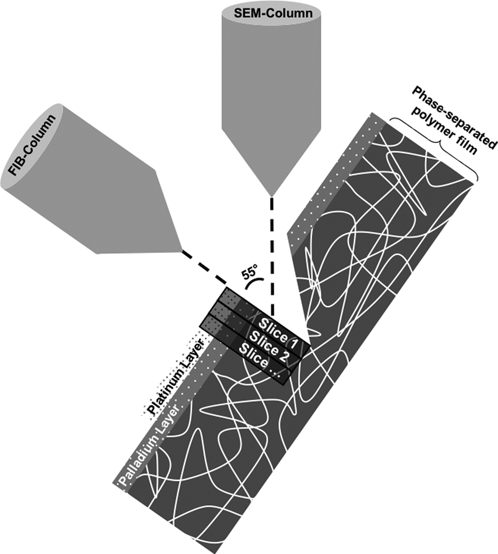
Fig. 1. The focused ion beam combined with a scanning electron microscope tomography setup. The palladium and platinum layers as well as the slicing direction are marked.
Preparation of Soft Materials
The first step toward 3D reconstructions of soft, porous, and poorly conducting materials is to prepare the specimen. Conventional specimen preparation techniques for soft materials to be imaged by SEM are, for example, staining of the specimen and/or using a variable-pressure scanning electron microscope (VP-SEM). The purpose of staining is to enhance the contrast and reduce charging. However, there is always a risk of introducing artifacts while staining the specimen. The VP-SEM also reduces charging. The disadvantage with the VP-SEM for the slice and imaging procedure is that the ion-beam milling is not possible in a gaseous specimen environment. We have, therefore, adopted a procedure that avoids staining and the use of VP-SEM. The specimen is mounted onto an aluminum stub with an adhesive carbon tape. If needed, silver glue can also be added to the stub to ensure the adhesion as well as increasing the conductivity. Deposition of a thin palladium layer onto the specimen surface is used to reduce the charging effects. In this work, an Emitech K550X Palladium Sputter (Quorum Technologies Ltd, Ashford, UK) was used with a coating current of 25 mA for 3 min while rotating the specimen holder. Other metals such as gold or tungsten can also be used.
Results and Discussion
Curtaining
Ion-beam milling can cause cross-sectioning artifacts such as curtaining (Giannuzi & Stevie, Reference Giannuzi and Stevie2005). Curtains are vertical lines visible in the cross section surface that are caused by the ion beam and can be seen in Figure 2a. Different hardness within a material or thickness can cause different ion milling rates which results in the curtaining.
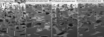
Fig. 2. SEM Mid-Angle BSE images showing cross sections of a soft porous polymer with different protective layers: (a) Charge-reducing palladium layer has been deposited, curtaining effect is highlighted by arrows. The top edge is also smeared. (b) Palladium layer and protective carbon layer, (c) palladium layer and protective tungsten layer, and d) palladium layer and protective platinum layer. Arrows in (b)–(d) point to the interface between the protective layers and the top surface. The smearing observed in (a) is absent in (b)–(d).
Reduce Curtaining by Optimization of Ion-Beam Parameters
Curtaining can be minimized, for example, by reduced milling rates (Giannuzi & Stevie, Reference Giannuzi and Stevie2005), where parameters that affect the milling rates are ion beam energy and current. We chose to operate at 30 keV and optimize the ion beam current to reduce curtaining. The results show that the cross-sectioning artifacts can all be avoided at 30 keV. The current is optimized by the following experimental approach. When milling the largest trench in the formation of the U shape, a current as high as possible without causing cross-sectioning artifacts is required in order to achieve time-efficient milling. The tuning of the highest beam current starts at 20 nA followed by a stepwise increase to find the optimized current, in our case 40 nA. Cross-sectioning artifacts are present here. However, these are removed in subsequent polishing of the cross section where lower beam currents are used. The other milling operations are optimized using the same approach, but starting at lower currents. The surface morphology is examined after each milling to find the highest current that does not cause cross-sectioning artifacts. In this study, the ion-beam parameters used for slicing are 1 nA and 30 keV.
Reduce Curtaining by Deposition of Protective Layer
The previous work has shown that the deposition of a protective platinum layer onto the specimen can be used to reduce the curtaining effect (Walley et al., Reference Walley, Wineberg and Burden1971; Suzuki, Reference Suzuki2002; Drobne et al., Reference Drobne, Milani, Leser and Tatti2007; Mayer et al., Reference Mayer, Giannuzzi, Kamino and Michael2007). A platinum gas precursor is injected into the chamber. The precursor is cleaved by the ion beam, which results in deposition of platinum. The platinum layer provides a dense, smooth surface that gives rise to a more uniform milling rate. In addition to platinum precursors, other gas precursors are available such as tungsten or carbon. Figure 2a shows a cross section where a few nanometer thin palladium layer has been deposited to reduce the charging effects. The arrow in Figure 2a points to curtains caused by the ion beam. It can also be seen that the top edge of the specimen is smeared. Figure 2b shows a cross section with the palladium layer, and carbon as a protective layer. The arrow points to the interface between the protective layer and the top surface of the specimen. Figure 2c shows a cross section with the palladium layer, and tungsten as a protective layer; and in Figure 2d, the protective platinum layer deposited on top of the palladium layer is visualized. The smearing observed in Figure 2a is absent in Figures 2b–2d. As can be seen, the different protective layers give different contrast. One advantage of the distinct contrast difference between the specimen and the protective layer is that it simplifies the image alignment procedure. The optimal protective layer to deposit depends on the material that is to be analyzed.
Charging
The accumulation of charge at the specimen surface is a common problem when imaging or milling soft materials. We have developed a protocol for imaging by optimizing the electron-beam parameters to reduce charging without staining or using a VP-SEM (Stokes, Reference Stokes2008).
Reduce Charging by Optimization of Electron-Beam Parameters
It is known that no charging of poorly conducting materials occurs when the number of primary electrons impinging on the surface is roughly equal to the number of electrons emitted from the specimen surface, that is, the total number of backscattered electrons (BSE) and secondary electrons (SE) (Goldstein et al., Reference Goldstein, Newbury, Joy, Lyman, Echlin, Lifshin, Sawyer and Michael2003). The beam energy influences the ratio between the number of incoming electrons and emitted electrons and, therefore, must be tuned to achieve the no-charging condition. There are two cross-over points, E 1 and E 2, where the primary beam energy gives an electron yield equal to 1. For soft materials, the low-energy cross-over point occurs in the energy range of 0.5–2 keV and the high-energy cross-over point occurs at 2–5 keV (Goldstein et al., Reference Goldstein, Newbury, Joy, Lyman, Echlin, Lifshin, Sawyer and Michael2003).
Specimen charging is reduced by fine-tuning the electron-beam parameters. This was carried out by varying the energy until as little charging as possible was noticed while sustaining sufficient detector signal. The initial electron beam energy was chosen to be 2 keV, based upon the rule of thumb that the primary beam energy for no charging of poorly conducting materials lies within 0.5–2 keV, depending on the material (Goldstein et al., Reference Goldstein, Newbury, Joy, Lyman, Echlin, Lifshin, Sawyer and Michael2003). Using this experimental approach, the optimized electron beam energy was found to be 700 eV (see Fig. 3b). Different electron beam energies were applied to find the optimized electron beam energy for imaging soft poorly conducting materials (see Fig. 3). If the electron beam energy was below 700 eV, less charging was observed. However, too poor signal was received (see Fig. 3a). If the electron beam energy was selected above 700 eV, the signal was improved (see Figs. 3c–3h). However, the accumulation of local charges was observed. This increased with decreasing scan rate and progression of time for the slice-and-image session. The next step was to optimize the electron beam current, which was achieved with the same approach as for the electron beam energy. The optimized current corresponded to the minimum available current in the instrument settings, which was 10 pA. Figure 4 shows results for the different applied currents that were used to find the optimal value.
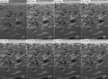
Fig. 3. Procedure used for selecting the optimised electron beam energy. Images recorded at energies ranging from (a) 0.5 keV to (h) 2 keV. The electron beam current was kept constant below 10 pA. The optimal electron beam energy was found to be 700 eV based both on the individual images and accumulation of charge during the slice-and-image session.
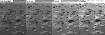
Fig. 4. Procedure for selecting electron beam current, ranging from (a) below 10 pA to (d) 265 pA. The electron beam energy was kept constant on 700 eV. The optimal current corresponded to the minimum beam current that could be used, which was 10 pA.
Reduce Charging by Charge Neutralization
The previous work has shown that localized charge neutralization can be achieved by the injection of nitrogen gas using a gas injection system (Schulz et al., Reference Schulz, Zeile, Stodolka and Kaft2009). This approach limits the volume of lower vacuum to that associated with a small specimen area of interest that can be imaged with reduced charging.
In this work, charge neutralization using carbon gas from the gas injection system was used to further reduce charging. Figure 5a shows where charging can be observed and Figure 5b shows when charge neutralization using carbon gas has been used and where no charging is observed. Cross-sectioning artifacts were present when carbon gas was injected during milling. Hence, the gas was only injected prior to the electron-beam imaging. The charge neutralization procedure was carried out as follows: Carbon gas was injected into the chamber for 5 sec by opening the carbon gas valve. The valve was closed after 5 sec where upon imaging with reduced charging could be performed. This procedure was incorporated in the automatic slice-and-imaging procedure by pausing after each slicing. Therefore, the slice-and-imaging procedure resulted in a semi-automatic procedure. It was found that the distance between the specimen and the valve opening played an important role. When the gas opening was too close to the specimen, carbon deposition occurred. The effect of the carbon deposition was evident through curtaining during subsequent milling. The curtaining appeared due to uneven carbon deposition caused by the sample orientation in the FIB–SEM chamber which was not optimal for the electron beam or ion beam deposition. Instead, the charge neutralization was achieved due to ionization of the gas molecules which in turn neutralized the charge accumulation at the cross-section surface. When the valve opening was too far away from the specimen, no charge neutralization occurred. The optimized distance was experimentally tried and found by retracting the valve for 10 sec from its inserted end position.
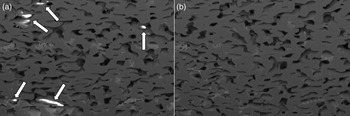
Fig. 5. (a) Cross section with charging where arrows indicate on the locally charged areas. (b) Cross section where charge neutralisation using carbon gas has been used. No charging observed.
Reduce Charging by Selection of Detector
A secondary electron detector is often selected when imaging conducting materials with low electron beam energy (Goldstein et al., Reference Goldstein, Newbury, Joy, Lyman, Echlin, Lifshin, Sawyer and Michael2003). However, when charging occurs, the SE are much more affected because of their low kinetic energy, less than 50 eV, compared to BSE. Thus, BSE are preferred when imaging poorly conducting materials. Figure 6a shows a cross section imaged using In-Beam SE where the arrows point to local charged areas. The same areas can be seen in Figure 6b without charging when imaged with the Mid-Angle BSE detector. It can be seen that the pore edges can more clearly be distinguished in the BSE image.
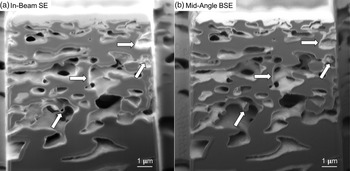
Fig. 6. (a) Cross section imaged using the In-Beam SE detector where the arrows are pointing to locally charged areas. (b) Cross section imaged using the Mid-Angle BSE detector where the arrows are pointing to the same areas as in (a) but without charging.
Redeposition and Shadowing Effects
Shadowing effects are caused by material surrounding the cross section, as shown in Figure 7a. Redeposition is caused by sputtered material that is deposited onto the specimen surface, often near or on top of the cross section, as illustrated in Figure 7b. In order to minimize these shadowing effects and redeposition, trenches on each side and in front of the cross section, in the form of a U shape was milled (Holzer et al., Reference Holzer, Indutnyi, Gasser, Much and Wegmann2004). Figure 7c shows a schematic overview of the steps involved to establish the U shape. The initial step is to deposit a protective platinum layer on the specimen surface to reduce the curtaining effect (see number 1 in Fig. 7c). A cross section is milled in order to reveal the internal porous microstructure followed by milling narrow trenches on each side of the cross section (see numbers 2 and 3 in Fig. 7c). In order to reveal the full cross-section surface, a bigger trench in front of the cross section is milled (see number 4 in Fig. 7c). Platinum is then deposited as two squares where fiducial markers (used to prevent drifting) are etched (see number 5 in Fig. 7c). The last step was to polish the cross section from curtaining and redeposition (see number 6 in Fig. 7c). This is also the starting point of the slice-and-image procedure.
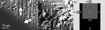
Fig. 7. (a) SEM Mid-Angle BSE image of a cross section where curtaining (arrow 1) and shadowing effects (arrow 2) are shown. (b) Redeposition on the cross section surface. (c) Schematic overview that shows the different steps required to establish a U shape. Number 1 represents deposition of a protective platinum layer, number 2 shows the location of the first cross section, number 3 represents the narrow trenches of the U shape, number 4 shows the big trench that reveals the full cross section surface, number 5 shows the location of the fiducial markers for the FIB and the SEM, and number 6 is the starting point of the slice-and-image procedure.
Beam Damage
Radiation damage is a factor limiting spatial resolution when imaging soft materials using electron microscopy (Egerton et al., Reference Egerton, Li and Malac2004; Egerton, Reference Egerton2013). When too high electron beam energy is used to image a soft porous and poorly conductive polymer, the material can be damaged. Figure 8 illustrates the image quality as a function of acceleration voltage in the range of 1–30 keV (see Figs. 8a–8g). The electron beam current is kept fixed at a higher value of 265 pA and the images are acquired using the Mid-Angle BSE. The effect of acceleration voltage is clearly visible when comparing the arrowed (1) pore in Figures 8a–8c. A charging artifact can be seen inside the arrowed (1) pore when the acceleration voltage is increased to 3 and 5 keV. It is also evident that the subsurface signal is increasing with increased acceleration voltage. It is difficult to distinguish the outline of the arrowed (1) pore at 30 keV (see Fig. 8g). The shape of the pore has changed after exposure to the high beam energy (see Fig. 8h). The beam damage causes a deformation that is observed all over the cross section (see arrows (2)). By comparing Figure 8a with Figure 8h, it can be seen that the soft material has been damaged by the electron beam as a result of the increased electron beam energy causing an inclination of the top surface. Figure 8h is recorded at the lower beam energy of 1 keV and it appears as though the inclination has been partially recovered from the state imaged at 30 keV. This implies that the deformation is partially reversible.
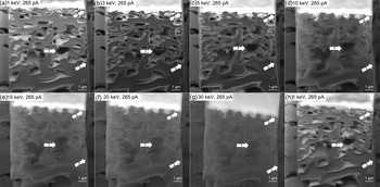
Fig. 8. Difference in surface sensitivity, and the effect of electron beam damage, when increasing the electron-beam energy from (a) 1 keV to (g) 30 keV with fixed current of 256 pA. (h) Cross section after the electron beam energy was increased. The arrowed (1) pore shows a charging artefact and the arrows (2) shows deformation caused by the effect of increased acceleration voltage.
Reconstruction
The 3D reconstruction of materials using FIB–SEM tomography is done by reconstructing binary 2D image stacks. After aligning and cropping the 2D image stacks, segmentation, that is, generating a binary map indicating solid (1) and pore (0), is performed (Joergensen et al., Reference Joergensen, Hansen, Larsen and Bowen2010). Conventional segmentation techniques, for example, global thresholding (Efford, Reference Efford2000), and more advanced segmentation algorithms, such as local thresholding, do not fully resolve this complex segmentation problem (Blayvas et al., Reference Blayvas, Bruckstein and Kimmel2006; Joergensen et al., Reference Joergensen, Hansen, Larsen and Bowen2010; Thiedmann et al., Reference Thiedmann, Hassfeld, Stenzel, Koster, Oosterhout, Van Bavel, Wienk, Loos, Janssen and Schmidt2011). The local threshold backpropagation method (Salzer et al., Reference Salzer, Spettl, Stenzel, Smått, Lindén, Manke and Schmidt2012), which is based on the detection of structures that disappear and subsequent thresholding, has been suggested in the case of overlapping intensities.
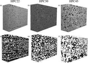
In this work, a method based on machine learning is presented. The 200 sequential 2D images obtained by FIB–SEM tomography were aligned and cropped to 3000 × 2000 pixels using the software ImageJ (Schneider et al., Reference Schneider, Rasband and Eliceriri2012), with the StackReg plugin and the Rigid Body method (which aligns images using translation and rotation operations). The 3D reconstruction of the specimen requires segmentation of the solid and pore phases in the 2D images. However, each 2D image contains subsurface information, that is, information about the structure in subsequent slices. This fact makes segmentation particularly challenging, for example, by introducing intensity overlaps. The first attempt used global thresholding (Efford, Reference Efford2000) for segmentation, but the results were found to be unsatisfactory with no clear distinction between the two phases. Instead, a method based on machine learning was used. First, manual segmentation was performed in 100 randomly placed square regions of size 256 × 256 pixels in each data set. This corresponds to approximately 0.5% of the full data set, but nevertheless took about 2 days to manually segment. Second, so-called linear scale-space features, that is, a set of Gaussian smoothed images at different scales, were extracted. Practically, this means that each slice was convolved with Gaussian filters, with standard deviations sigma = 1, 2, 4, 8, 16, 32, 64, and 128 pixels. This was performed for the slice to be segmented and for five adjacent slices in each direction. For the slice of interest, also the raw image intensity (unfiltered, corresponding to sigma = 0) was used. Hence, for each pixel to be classified, 89 features were extracted. The rationale for taking information from adjacent slices into account is that, because of the subsurface information, it is difficult to discriminate the pore and the matrix only using information from the slice of interest. A so-called random forest classifier was trained to perform classification into one of two possible classes, matrix or pore (Breiman, Reference Breiman2001). The random forest classifier combines the output of (in this case) 101 decision tree classifiers, producing a probability map that can be interpreted as the likelihood of the pixel of interest to belong to a pore or to the matrix. This probability map is smoothed and thresholded to yield a binary segmentation. After training on the available manually segmented data, the classifier was subsequently used for segmentation of the full data set. The 3D reconstructions were done by importing the binary 2D image stacks into the software ORS Visual (Object Research Systems (ORS), 2018, Montreal, Canada). Figures 9a–9c show SEM Mid-Angle BSE image stacks of three specimens with different porosities, and Figures 9d–9f show the corresponding 3D reconstructions of the porous network in white.

Fig. 9. SEM Mid-Angle BSE image stacks of three specimens with different porosities with the width (x): 30 µm, height (y): 20 µm and depth (z): 10 µm where (a) HPC22 with the lowest porosity, (b) HPC30 with intermediate porosity and (c) HPC45 with the highest porosity. The corresponding 3D porous network in each specimen is shown reconstructed in white in (d) HPC22, (e) HPC30 and (f) HPC45.
Conclusion
A general protocol for optimization of FIB–SEM tomography parameters for porous and poorly conducting soft materials has been described. The protocol includes the reduction of curtaining, redeposition, shadowing effects, and charging. In addition, it handles the subsurface and grayscale intensity overlap problems in the image segmentation for 3D reconstruction.
The curtaining is reduced by optimization of the ion beam current as well as deposition of a protective platinum layer. The shadowing effects and redeposition are removed by milling a U shape. The charging problem is solved by optimizing of the electron beam energy and current, coating the specimen with palladium, deposition of a protective platinum layer, charge reduction using a carbon gas, as well as choosing the most appropriate detector. The subsurface information and intensity overlap in the images give rise to complications during segmentation of the data. It was found that a machine learning-based random forest approach is able to automatically segment the data and differentiate between the solid material and pores.
We evaluated the protocol by optimizing FIB–SEM tomography parameters for phase-separated and leached ethyl cellulose/hydroxypropyl cellulose films having both poor conductivity and pores. 3D reconstructions of three films with different porosities were successfully obtained.
Acknowledgments
The authors gratefully acknowledge the Swedish Foundation for Strategic Research (SSF) project “Material structures seen through microscopes and statistics” and the Area of Advance Materials Science at the Chalmers University of Technology for funding this work, AstraZeneca for providing the material and Chalmers Material Analysis Laboratory for their support of microscopes. Furthermore, we gratefully acknowledge Sandra Barman and Holger Rootzén for valuable discussions.


 Open access