


1. Introduction
The motion of a particle in a dilute suspension depends primarily on its interaction with a background flow rather than on interactions with other particles. As one application, understanding the dynamics of small particles in various flows is necessary to understand the dispersion of suspensions. For example, a particle's shape can cause cross-streamline migration in Poiseuille flows (Chan & Leal Reference Chan and Leal1979; Leal Reference Leal1980; Nitsche & Hinch Reference Nitsche and Hinch1997; Jendrejack et al. Reference Jendrejack, Schwartz, de Pablo and Graham2004; Słowicka, Wajnryb & Ekiel-Jeżewska Reference Słowicka, Wajnryb and Ekiel-Jeżewska2013; Farutin et al. Reference Farutin, Piasecki, Słowicka, Misbah, Wajnryb and Ekiel-Jeżewska2016) or aid in separation of particles, either through chirality (Kim & Rae Reference Kim and Rae1991; Marcos, Powers & Stocker Reference Marcos, Powers and Stocker2009; Ro, Yi & Kim Reference Ro, Yi and Kim2016; Witten & Diamant Reference Witten and Diamant2020) or asymmetry of shape (Lopez & Graham Reference Lopez and Graham2007; Masaeli et al. Reference Masaeli, Sollier, Amini, Mao, Camacho, Doshi, Mitragotri, Alexeev and Di Carlo2012; Berthet, Fermigier & Lindner Reference Berthet, Fermigier and Lindner2013; Uspal, Eral & Doyle Reference Uspal, Eral and Doyle2013; Bet et al. Reference Bet, Samin, Georgiev, Eral and van Roij2018). Shape can also affect the dispersion of particles in flows of suspensions, either by altering diffusive properties (Han et al. Reference Han, Alsayed, Nobili, Zhang, Lubensky and Yodh2006; Chakrabarty et al. Reference Chakrabarty, Konya, Wang, Selinger, Sun and Wei2013; Koens, Lisicki & Lauga Reference Koens, Lisicki and Lauga2017) or affecting Taylor dispersion in pipe flows (Taylor Reference Taylor1954; Kumar et al. Reference Kumar, Thomson, Powers and Harris2021). Many relevant flows in microfluidic and other applications, such as Poiseuille or Couette flows, are approximately a shear flow at sufficiently small scales. Therefore, it is useful to understand the behaviour of different classes of small particles in a simple shear flow at low Reynolds numbers in order to understand the behaviour of suspensions of these particles in various engineering applications.
Slender particles or shapes are found in a range of examples in nature and industry, for example as flagella used for biological propulsion (Keller & Rubinow Reference Keller and Rubinow1976b; Lighthill Reference Lighthill1976; Lauga & Powers Reference Lauga and Powers2009; De Canio, Lauga & Goldstein Reference De Canio, Lauga and Goldstein2017), biological (Kantsler & Goldstein Reference Kantsler and Goldstein2012) and artificial filaments (Pawłowska et al. Reference Pawłowska, Nakielski, Pierini, Piechocka, Zembrzycki and Kowalewski2017; Nunes et al. Reference Nunes, Li, Griffiths, Rallabandi, Man and Stone2021), and polymers (Smith, Babcock & Chu Reference Smith, Babcock and Chu1999). By definition, these objects have a small aspect ratio, defined as the ratio of the particle's characteristic cross-sectional radius to its length. This feature allows their dynamics to be well-approximated by either slender-body theory (Batchelor Reference Batchelor1970; Cox Reference Cox1970; Johnson Reference Johnson1980) or the similar resistive force theory (Gray & Hancock Reference Gray and Hancock1955; Keller & Rubinow Reference Keller and Rubinow1976a). Slender particles in a pipe flow have been shown to have increased axial dispersion (Kumar et al. Reference Kumar, Thomson, Powers and Harris2021) as well as a tendency to migrate across streamlines (Nitsche & Hinch Reference Nitsche and Hinch1997; Słowicka et al. Reference Słowicka, Ekiel-Jeżewska, Sadlej and Wajnryb2012, Reference Słowicka, Wajnryb and Ekiel-Jeżewska2013; Farutin et al. Reference Farutin, Piasecki, Słowicka, Misbah, Wajnryb and Ekiel-Jeżewska2016) driven by the interaction of their narrow shape with a given flow and the confining boundaries.
Shapes with high symmetry tend to have relatively simple dynamics in low-Reynolds-number flow. For example, a general axisymmetric ellipsoid placed in a simple shear flow tumbles periodically (Jeffery Reference Jeffery1922). This tumbling motion is characterized by unique orbits, called Jeffery orbits, which are parameterized solely by the particle's initial orientation relative to the flow. The period with which the particle completes an orbit is a function of the particle's aspect ratio. Straight slender objects undergo Jeffery orbits with very long periods (Cox Reference Cox1971) and any axisymmetric object in a shear flow will follow a Jeffery orbit, which may be classified in terms of an ‘equivalent’ ellipsoid (Bretherton Reference Bretherton1962).
Brenner (Reference Brenner1963) demonstrated that it is possible to construct objects that will adopt stable orientations with respect to a three-dimensional shear flow, and can be accompanied by persistent drift across streamlines. Shapes with these dynamics may be constructed that are either asymmetric or bodies of revolution. The defining characteristic of such shapes is that their aspect ratio is very small. This allows the body to experience two very different regions of the flow, which can lead to such stable equilibrium dynamics. Bretherton (Reference Bretherton1962) considers shapes that are either arrays of spheres and ellipsoids or more complex bodies of revolution. Borker, Stroock & Koch (Reference Borker, Stroock and Koch2018) extended this work to consider the equilibrium dynamics of the bodies of revolution, illustrating the dependence of the equilibrium dynamics on the body's cross-section.
As the constraint of axisymmetry on a particle's shape is relaxed, more complicated dynamics become possible. For example, a triaxial ellipsoid will experience chaotic Jeffery orbits in which the orbital constant is no longer fixed by the initial orientation (Hinch & Leal Reference Hinch and Leal1979; Yarin, Gottlieb & Roisman Reference Yarin, Gottlieb and Roisman1997). Also, when slender filaments deform elastically in shear flow they experience tumbling motions similar to a Jeffery orbit but with orbital constants that decay or grow exponentially with time (Słowicka, Stone & Ekiel-Jeżewska Reference Słowicka, Stone and Ekiel-Jeżewska2020) as well as experiencing other bending, curling and rotational dynamics (du Roure et al. Reference du Roure, Lindner, Nazockdast and Shelley2019; Zuk et al. Reference Zuk, Słowicka, Ekiel-Jeżewska and Stone2021).
As many slender particles in nature and engineering processes are curved, due in part to the prevalence of elastic slender particles, the previous results suggest that they may have more complex dynamics than a Jeffery orbit. Recent work has shown that, in a simple shear flow, rigid, curved slender bodies that possess a plane of reflectional symmetry undergo chaotic orbits (Thorp & Lister Reference Thorp and Lister2019) and persistent cross-streamline drift (Wang et al. Reference Wang, Tozzi, Graham and Klingenberg2012) depending on the particle's shape and initial orientation. This behaviour is due to a lack of symmetry in the particle's orientation as it rotates in three dimensions (Thorp & Lister Reference Thorp and Lister2019). A consequence of the cross-streamline drift is enhanced dispersion of the particles (Wang, Graham & Klingenberg Reference Wang, Graham and Klingenberg2014).
We continue the exploration of slender particle motion in shear flow by considering asymmetrically bent, rigid slender bodies. In particular, we study an asymmetric boomerang shape, consisting of two rods of varying length joined end-to-end with a variable angular offset. Composite bodies of straight slender rods qualitatively capture the dynamics of more complex curvatures (De Canio et al. Reference De Canio, Lauga and Goldstein2017) and so this shape is analogous to a curved body. We choose to focus on this shape as most curved particles in nature do not possess reflectional symmetry, such that they are not simply sections of a circle. As previous studies have shown, even minor reductions in a particle's symmetry can have major effects on the dynamics.
We consider the asymmetric boomerang confined to a plane perpendicular to the flow's vorticity. Recent papers examine similarly restricted particle motion in microfluidic channels (Georgiev et al. Reference Georgiev, Toscano, Uspal, Bet, Samin, van Roij and Eral2020) or for flexible fibres (Słowicka, Wajnryb & Ekiel-Jeżewska Reference Słowicka, Wajnryb and Ekiel-Jeżewska2015) while others have studied the two-dimensional diffusivity of symmetric boomerangs (Chakrabarty et al. Reference Chakrabarty, Konya, Wang, Selinger, Sun and Wei2013; Koens et al. Reference Koens, Lisicki and Lauga2017). Others have studied the gravitaxis (ten Hagen et al. Reference ten Hagen, Kümmel, Wittkowski, Takagi, Löwen and Bechinger2014) and self-propulsion (ten Hagen et al. Reference ten Hagen, Wittkowski, Takagi, Kümmel, Bechinger and Löwen2015) of similar asymmetric boomerangs as well as the Brownian motion of asymmetric, complex shapes (Cichocki, Ekiel-Jezewska & Wajnryb Reference Cichocki, Ekiel-Jezewska and Wajnryb2012; Kraft et al. Reference Kraft, Wittkowski, Hagen, Edmond, Pine and Löwen2013; Cichocki, Ekiel-Jezewska & Wajnryb Reference Cichocki, Ekiel-Jezewska and Wajnryb2017). We expect that such a particle would have interesting dynamics, as the boomerang becomes a two-dimensional analogue of the ellipsoidal array proposed in figure 5 of Bretherton (Reference Bretherton1962) for high degrees of asymmetry. However, the shape we consider is much simpler and more likely to be seen in a natural setting than the arrays discussed by Bretherton (Reference Bretherton1962). By focusing on the particle's behaviour in a plane we may proceed analytically using first-order slender-body theory and find new features of the dynamics due to the shape of the particle without the complications of chaotic orbital dynamics. Thus, we are able to show that particle drift transverse to the streamlines can result from shape alone instead of requiring asymmetry in tumbling motions.
We first present in § 2 a theoretical discussion of the motion of a general body confined to a two-dimensional shear flow. We show that particles will either undergo tumbling motion with periodic cross-streamline motion of the centre of mass, consistent with the ‘scooping’ observed by Wang et al. (Reference Wang, Tozzi, Graham and Klingenberg2012), or will adopt a fixed orientation and drift across streamlines. We provide the geometric condition that determines the dynamics of the particle. We next consider in § 3 the asymmetric boomerang shape and compute which variations of the shape enable persistent drifting motion. We analyse the characteristics of the drift and show that while it results from a different mechanism than previously identified in the literature, it is consistent in magnitude with the cross-streamline drift previously observed for symmetric shapes. Finally, we discuss some features of the particle's motion in both the fixed (§ 3.2) and periodically rotating regimes (§ 3.3).
2. Motion of particles in shear flow
The Reynolds number  $Re$ characterizes the motion of a fluid with viscosity $\mu$, density $\rho$ and characteristic velocity $U$ around an immersed body of characteristic length $L$, and is defined as $Re = \rho U L /\mu$. For $Re\ll 1$, and an incompressible flow of a Newtonian fluid, the fluid stress $\boldsymbol {\sigma }$, pressure $p$ and velocity $\boldsymbol {u}$ of the flow are well-approximated by the Stokes equations,
 $$\begin{gather} \boldsymbol{\nabla}\boldsymbol{\cdot}\boldsymbol{\sigma} ={-} \boldsymbol{\nabla}p + \mu \nabla^2 \boldsymbol{u} = {\boldsymbol 0}, \end{gather}$$
 $$\begin{gather}\boldsymbol{\nabla}\boldsymbol{\cdot}\boldsymbol{u} = 0. \end{gather}$$
An arbitrary flow linear in position  $\boldsymbol {x}$ can be decomposed into a constant component $\boldsymbol {U}^\infty$, a rotational component due to the vorticity of the flow $\boldsymbol {\omega }^\infty$ and a rate-of-strain component ${\boldsymbol{\mathsf{E}}}^\infty$ as
 \begin{equation} \boldsymbol{u}^\infty (\boldsymbol{x})= \boldsymbol{U}^\infty + \tfrac{1}{2}\boldsymbol{\omega}^\infty \wedge \boldsymbol{x} + {\boldsymbol{\mathsf{E}}}^\infty\boldsymbol{\cdot}\boldsymbol{x}.\end{equation}
Note that this decomposition satisfies (2.1) and (2.2). The decomposition of a shear flow with shear rate  $\dot {\gamma }$, $\boldsymbol {u}^\infty (\boldsymbol {x}) = \dot {\gamma }y \boldsymbol {e}_1'$, is depicted in figure 1. In a shear flow, vorticity and the rate-of-strain balance to cancel out vertical motion and produce horizontal velocity that varies linearly with the vertical coordinate $y$.
$y$.

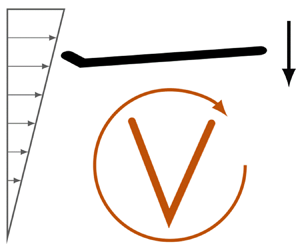
Figure 1. Decomposition of a linear shear flow into a rotational component and a rate-of-strain component. The shear flow  $\boldsymbol {u}^\infty (\boldsymbol {x}) = \dot {\gamma }y\boldsymbol {e}_1'$ may be written as $\boldsymbol {u}^\infty (\boldsymbol {x}) = \frac {1}{2}\boldsymbol {\omega }^\infty \wedge \boldsymbol {x} + {\boldsymbol{\mathsf{E}}}^\infty \boldsymbol {\cdot } \boldsymbol {x}$, where the values of $\boldsymbol {\omega }^\infty$ and ${\boldsymbol{\mathsf{E}}}^\infty$ are given in the figure relative to the $\boldsymbol {e}_1'-\boldsymbol {e}_2'-\boldsymbol {e}_3'$ laboratory reference frame. The dynamics of the particle in the shear flow is a linear combination of the particle's dynamics in each component flow. The flow decomposition for particles whose centre does not fall on $y=0$ will also include a constant velocity translation, $\boldsymbol {U}^\infty$, in the direction of the shear, as the decomposition into rotational and extensional components assumes that the particle's centre is located at $\boldsymbol {x}=\boldsymbol {0}$. However, for force and torque-free particles, $\boldsymbol {U}^\infty$ will serve only to advect the particle downstream.
A rigid particle, with domain  $V$ and surface $S$, immersed in a flow will undergo a rigid body translational $( \boldsymbol {U} )$ and rotational $( \boldsymbol {\varOmega } )$ motion described by
 \begin{equation} \boldsymbol{u}_{body}(\boldsymbol{x}\in V) = \boldsymbol{U} + \boldsymbol{\varOmega}\wedge \boldsymbol{x}, \end{equation}
where  $\boldsymbol {\varOmega }$ changes the particle's orientation. The solution to the flow problem is a velocity field that produces hydrodynamic stresses that exactly balance any external forces or torques acting on the particle.
2.1. Resistance and mobility tensors
The resistance problem deals with determining the hydrodynamic force  $\boldsymbol {F}$, torque $\boldsymbol {T}$ and stresslet ${\boldsymbol{\mathsf{S}}}$ exerted by a fluid on a particle as a function of the particle's motion. These quantities may be determined by integrating the fluid stress $\boldsymbol {\sigma }$ over the surface of the particle.
As a result of the linearity of the governing equations, (2.1) and (2.2), and the external flow, (2.3), the contributions of the flow's constant, rotational and straining components may be calculated individually. Dimensional analysis then sets the relationship between the motion and the hydrodynamics as (Brenner Reference Brenner1963; Happel & Brenner Reference Happel and Brenner1983; Kim & Karrila Reference Kim and Karrila1991, chapter 5)
 \begin{equation} \begin{bmatrix} \boldsymbol{F}\\ \boldsymbol{T}\\ {\boldsymbol{\mathsf{S}}} \end{bmatrix} = \mu \begin{bmatrix} {\boldsymbol{\mathsf{A}}} & \tilde{{\boldsymbol{\mathsf{B}}}} & \tilde{{\boldsymbol{\mathsf{G}}}} \\ {\boldsymbol{\mathsf{B}}} & {\boldsymbol{\mathsf{C}}} & \tilde{{\boldsymbol{\mathsf{H}}}} \\ {\boldsymbol{\mathsf{G}}} & {\boldsymbol{\mathsf{H}}} & {\boldsymbol{\mathsf{M}}} \\ \end{bmatrix} \boldsymbol{\cdot} \begin{bmatrix} \boldsymbol{U}^\infty - \boldsymbol{U} \\ \tfrac{1}{2}\boldsymbol{\omega}^\infty - \boldsymbol{\varOmega} \\ {\boldsymbol{\mathsf{E}}}^\infty \\ \end{bmatrix},\end{equation}
where  ${\boldsymbol{\mathsf{A}}}$, ${\boldsymbol{\mathsf{B}}}$ and ${\boldsymbol{\mathsf{C}}}$ are second-order tensors, ${\boldsymbol{\mathsf{G}}}$ and ${\boldsymbol{\mathsf{H}}}$ are third-order tensors and ${\boldsymbol{\mathsf{M}}}$ is a fourth-order tensor, which collectively are known as the grand resistance tensor. The tilde notation follows that defined by Kim & Karrila (Reference Kim and Karrila1991, chapter 5); e.g. for second-rank tensors $\textsf{{B}}_{ij}=\tilde {\textsf{{B}}}_{ji}$ while for third-rank tensors $\textsf{{G}}_{ijk} = \tilde {\textsf{{G}}}_{kij}$. The grand resistance tensor is usually written in a reference frame fixed to the particle, so that the values of the resistance coefficients remain constant even as the particle's orientation changes. The grand resistance tensor is symmetric and positive definite; this fact was proved for the force and torque relationships by Happel & Brenner (Reference Happel and Brenner1983) and then more generally for the entire grand resistance tensor by Hinch (Reference Hinch1972) (see also Kim & Karrila (Reference Kim and Karrila1991), chapter 5).
The inverse to the resistance problem is known as the mobility problem. One may similarly define a grand mobility tensor as
 \begin{equation} \begin{bmatrix} \boldsymbol{U}-\boldsymbol{U}^\infty \\ \boldsymbol{\varOmega}-\tfrac{1}{2}\boldsymbol{\omega}^\infty \\ -\mu^{{-}1}{\boldsymbol{\mathsf{S}}} \\ \end{bmatrix} = \begin{bmatrix} {\boldsymbol{\mathsf{a}}} & \tilde{{\boldsymbol{\mathsf{b}}}} & \tilde{{\boldsymbol{\mathsf{g}}}} \\ {\boldsymbol{\mathsf{b}}} & {\boldsymbol{\mathsf{c}}} & \tilde{{\boldsymbol{\mathsf{h}}}} \\ {\boldsymbol{\mathsf{g}}} & {\boldsymbol{\mathsf{h}}} & {\boldsymbol{\mathsf{m}}} \\ \end{bmatrix} \boldsymbol{\cdot} \begin{bmatrix} \mu^{{-}1}\boldsymbol{F}\\ \mu^{{-}1}\boldsymbol{T}\\ {\boldsymbol{\mathsf{E}}}^\infty \end{bmatrix}.\end{equation}
For convenience in subsequent work, we have adopted the opposite sign convention for the mobility tensor to that used by Kim & Karrila (Reference Kim and Karrila1991, chapter 5). The choice of sign is arbitrary and only effects the relationships between the resistance and mobility coefficients. In practice, it is usually easier to calculate resistance coefficients for a given body and then use these to calculate the mobility coefficients rather than directly determining the mobility coefficients from the shape. Using our sign convention, the components of the grand mobility tensor relevant to this work are related to the components of the grand resistance tensor by
 \begin{equation} \begin{bmatrix} \tilde{{\boldsymbol{\mathsf{g}}}} \\ \tilde{{\boldsymbol{\mathsf{h}}}} \\ \end{bmatrix} = \begin{bmatrix} {\boldsymbol{\mathsf{A}}} & \tilde{{\boldsymbol{\mathsf{B}}}} \\ {\boldsymbol{\mathsf{B}}} & {\boldsymbol{\mathsf{C}}} \\ \end{bmatrix}^{{-}1} \boldsymbol{\cdot} \begin{bmatrix} \tilde{{\boldsymbol{\mathsf{G}}}} \\ \tilde{{\boldsymbol{\mathsf{H}}}} \\ \end{bmatrix}.\end{equation}
Additional relationships for the remaining mobility coefficients in terms of the resistance coefficients may be found in Kim & Karrila (Reference Kim and Karrila1991, chapter 5) with the opposite sign than that used here.
2.1.1. Extensional flow
A general rate-of-strain  ${\boldsymbol{\mathsf{E}}}^\infty$ is a second-order tensor with nine components, but only five are independent due to the constraints of symmetry, $\textsf{{E}}^\infty _{ij}= \textsf{{E}}^\infty _{ji}$, and incompressibility, $\textsf{{E}}^\infty _{ii} = 0$. Therefore, one possible basis for a general straining flow is
 \begin{align} \left.\begin{array}{c@{}} {\boldsymbol{\mathsf{E}}}^{(1)} = \begin{bmatrix} 1 & 0 & 0 \\ 0 & -1 & 0 \\ 0 & 0 & 0 \\ \end{bmatrix} , \quad {\boldsymbol{\mathsf{E}}}^{(2)} = \begin{bmatrix} 0 & 1 & 0 \\ 1 & 0 & 0 \\ 0 & 0 & 0 \\ \end{bmatrix} , \quad {\boldsymbol{\mathsf{E}}}^{(3)} = \begin{bmatrix} -1 & 0 & 0 \\ 0 & -1 & 0 \\ 0 & 0 & 2 \\ \end{bmatrix},\\ {\boldsymbol{\mathsf{E}}}^{(4)} = \begin{bmatrix} 0 & 0 & 1 \\ 0 & 0 & 0 \\ 1 & 0 & 0 \\ \end{bmatrix}, \quad {\boldsymbol{\mathsf{E}}}^{(5)} = \begin{bmatrix} 0 & 0 & 0 \\ 0 & 0 & 1 \\ 0 & 1 & 0 \\ \end{bmatrix},\end{array}\right\} \end{align}
so that a straining flow may be expressed using this basis as (Kim & Karrila Reference Kim and Karrila1991, chapter 5):
 \begin{equation} {\boldsymbol{\mathsf{E}}}^\infty = \tfrac{1}{2}(E_{xx} - E_{yy}) {\boldsymbol{\mathsf{E}}}^{(1)} + E_{xy}{\boldsymbol{\mathsf{E}}}^{(2)} + \tfrac{1}{2}E_{zz} {\boldsymbol{\mathsf{E}}}^{(3)} + E_{xz}{\boldsymbol{\mathsf{E}}}^{(4)} + E_{yz}{\boldsymbol{\mathsf{E}}}^{(5)}. \end{equation}
Note that the first two terms are two-dimensional, confined to the  $x$–
$x$– $y$ plane while the final three terms involve flow in the $\boldsymbol {e}_z$ direction.
2.1.2. A convenient form of the rate-of-strain flow resistance and mobility coefficients
Due to the constraints of symmetry and incompressibility on the form of rate-of-strain flows that lead to the general form of an extensional flow in (2.8), the third-order resistance tensors  $\tilde {{\boldsymbol{\mathsf{G}}}}$ and $\tilde {{\boldsymbol{\mathsf{H}}}}$ are reduced from each having 27 independent components to only 15 independent components each. Further, it is possible to express a general straining flow ${\boldsymbol{\mathsf{E}}}^\infty$ as a five-component vector, $\boldsymbol {E}^\infty = [E_1^\infty, E_2^\infty, E_3^\infty, E_4^\infty, E_5^\infty ]^T$, where each component of the vector is the coefficient of the corresponding basis term in (2.8), e.g. $E_1^\infty = \frac {1}{2}(E_{xx}-E_{yy})$, $E_2^\infty = E_{xy}$, etc. Note that $\boldsymbol {E}^\infty$ represents a vector quantity to be distinguished from the rate-of-strain tensor ${\boldsymbol{\mathsf{E}}}^\infty$.
Using these facts it is convenient to define new second-rank resistance tensors  $\hat {{\boldsymbol{\mathsf{G}}}}$ and $\hat {{\boldsymbol{\mathsf{H}}}}$ which relate the vector form of straining flow to the force and torque acting on a rigid particle. These new tensors are equivalent to the standard third-rank form,
 \begin{equation} \begin{bmatrix} \tilde{{\boldsymbol{\mathsf{G}}}} \\ \tilde{{\boldsymbol{\mathsf{H}}}} \end{bmatrix} \boldsymbol{\cdot} {\boldsymbol{\mathsf{E}}}^\infty = \begin{bmatrix} \hat{{\boldsymbol{\mathsf{G}}}} \\ \hat{{\boldsymbol{\mathsf{H}}}} \end{bmatrix} \boldsymbol{\cdot} \boldsymbol{E}^\infty = \begin{bmatrix} \hat{{\boldsymbol{\mathsf{G}}}} \\ \hat{{\boldsymbol{\mathsf{H}}}} \end{bmatrix} \boldsymbol{\cdot} [\begin{array}{@{}ccccc@{}} E_1^\infty & E_2^\infty & E_3^\infty & E_4^\infty & E_5^\infty \end{array}]^T,\end{equation}
but are second-rank tensors with dimensions of three by five and 15 components each. In many cases, such as when using slender-body theory, it is more convenient to calculate the components of  $\hat {{\boldsymbol{\mathsf{G}}}}$ and $\hat {{\boldsymbol{\mathsf{H}}}}$ than to resolve the individual, non-independent components of $\tilde {{\boldsymbol{\mathsf{G}}}}$ and $\tilde {{\boldsymbol{\mathsf{H}}}}$.
Similarly, we may define two new mobility tensors  $\hat {{\boldsymbol{\mathsf{g}}}}$ and $\hat {{\boldsymbol{\mathsf{h}}}}$ that are equivalent to the full third-rank forms,
 \begin{equation} \begin{bmatrix} \tilde{{\boldsymbol{\mathsf{g}}}} \\ \tilde{{\boldsymbol{\mathsf{h}}}} \end{bmatrix} \boldsymbol{\cdot} {\boldsymbol{\mathsf{E}}}^\infty = \begin{bmatrix} \hat{{\boldsymbol{\mathsf{g}}}} \\ \hat{{\boldsymbol{\mathsf{h}}}} \end{bmatrix} \boldsymbol{\cdot} \boldsymbol{E}^\infty.\end{equation}
See Appendix A for a derivation of the components of  $\hat {{\boldsymbol{\mathsf{g}}}}$ in terms of the components of the original third-rank mobility tensor. The relationship between these second-rank forms of the straining flow mobility and resistance tensors is given by (2.7) with a substitution of $\hat {{\boldsymbol{\mathsf{g}}}}$ for $\tilde {{\boldsymbol{\mathsf{g}}}}$, and so forth. A proof of this relationship is presented in Appendix B.
2.2. Motion in two-dimensional shear flow
To consider the motion of particles in a shear flow, we define laboratory and particle reference frames in figure 2. The background shear flow is expressed as  $\boldsymbol {u}^\infty (\boldsymbol {x}) = \dot {\gamma }y\boldsymbol {e}_1'$. Torques on the particle are calculated about the particle's origin $O$. Vectors in the laboratory frame may be expressed in the particle's reference frame with the aid of a time-dependent rotation tensor ${\boldsymbol{\mathsf{R}}}$ as
 \begin{equation} \boldsymbol{x} = {\boldsymbol{\mathsf{R}}} \boldsymbol{\cdot} \boldsymbol{x}'. \end{equation}
Figure 2. The laboratory reference frame for a shear flow is defined such that  $\boldsymbol {e}_1'$ is parallel to the streamlines, $\boldsymbol {e}_2'$ is parallel to the flow's gradient and $\boldsymbol {e}_3'$ is parallel to the vorticity. In this frame, a shear flow is written as $\boldsymbol {u}^\infty (\boldsymbol {x}) = \dot {\gamma }y\boldsymbol {e}_1'$. We also define a particle-fixed reference frame where the particle's axes, $\{\boldsymbol {e}_1, \boldsymbol {e}_2, \boldsymbol {e}_3 \}$ are defined conveniently for the particular geometry relative to some origin $O$. For a two-dimensional flow, the particle's $\boldsymbol {e}_3$ axis is defined such that $\boldsymbol {e}_3' = \boldsymbol {e}_3$, which allows the rotation angle $\theta (t)$ to completely describe the relationship between the two frames. For a particle where point $O$ does not fall on $y=0$ for the shear flow, it is possible to subtract a uniform background flow $\boldsymbol {U}^\infty$ to create the situation illustrated. For a force-free and couple-free particle, this background flow merely advects the particle downstream but does not affect the rotational dynamics.
We will restrict our study to a consideration of systems of particles with sufficient symmetry with respect to their orientation in the flow such that the dynamics may be treated as two-dimensional. The effect of this symmetry is to ensure that a particle, which is initially oriented relative to the flow such that  $\boldsymbol {e}_3 = \boldsymbol {e}_3'$, will not experience any rotational motion except in the $\boldsymbol {e}_3'$ direction. This results in a particle never changing its orientation relative to the $\boldsymbol {e}_1'-\boldsymbol {e}_2'$ plane, which in turn means that the dynamics are two-dimensional. In terms of the components of the resistance tensors, such a particle must have coupling coefficients $\tilde {\textsf{{B}}}_{11}= \tilde {\textsf{{B}}}_{12}=\tilde {\textsf{{B}}}_{22}= \hat {\textsf{{G}}}_{3j}=\hat {\textsf{{H}}}_{1j}=\hat {\textsf{{H}}}_{2j}=0$ for $j =1,2,3,4,5$.
For such two-dimensional dynamics, the angle  $\theta (t)$ (see figure 2) is sufficient to relate the two reference frames through the tensor
 \begin{equation} {\boldsymbol{\mathsf{R}}} = \begin{bmatrix} \cos \theta & \sin \theta & 0 \\ -\sin\theta & \cos \theta & 0 \\ 0 & 0 & 1 \\ \end{bmatrix}.\end{equation}
 In this confined system, the general form of the grand resistance tensor, (2.5), reduces to three translational coefficients, one rotational coefficient, and two coupling coefficients relating the translational and rotational velocities to the force and torque (Koens et al. Reference Koens, Lisicki and Lauga2017). Furthermore, the straining component is a linear combination of only the basis matrices  ${\boldsymbol{\mathsf{E}}}^{(1)}$ and ${\boldsymbol{\mathsf{E}}}^{(2)}$ (see (2.8)). We may write any two-dimensional extensional flow as
 \begin{equation} {\boldsymbol{\mathsf{E}}}^\infty = E_1^\infty {\boldsymbol{\mathsf{E}}}^{(1)} + E_2^\infty {\boldsymbol{\mathsf{E}}}^{(2)}, \end{equation}
or, in terms of the vector notation introduced in § 2.1.2 as  $\boldsymbol {E}^\infty = [E_1^\infty,\,E_2^\infty ]^T$. This restriction on the form of $\boldsymbol {E}^\infty$, along with the conditions on the form of the coupling tensors, reduces the mobility tensors $\hat {{\boldsymbol{\mathsf{g}}}}$ and $\hat {{\boldsymbol{\mathsf{h}}}}$ to four and two components, respectively.
Neglecting the stresslet term, which has no effect on the particle's dynamics, and making use of the notation defined above, we write the two-dimensional equivalent of (2.6) for a force-free and torque-free particle as
 \begin{equation} \begin{bmatrix} U_1 - U_1^\infty \\ U_2 - U_2^\infty \\ \varOmega_3 - \tfrac{1}{2}\omega_3^\infty \\ \end{bmatrix} = \begin{bmatrix} \hat{g}_{11} & \hat{g}_{12} \\ \hat{g}_{21} & \hat{g}_{22} \\ \hat{h}_{31} & \hat{h}_{32} \\ \end{bmatrix} \boldsymbol{\cdot} \begin{bmatrix} E^\infty_{1} \\ E^\infty_{2} \\ \end{bmatrix}.\end{equation}
In the absence of a straining flow, a force and torque-free particle will rotate with the vorticity of, and be advected by, the background flow. It is a rigid particle's resistance to straining that gives rise to dynamics in excess of advection of the centre of mobility. For the bodies of interest in our problem we complete the derivation of  $\hat {{\boldsymbol{\mathsf{g}}}}$ and $\hat {{\boldsymbol{\mathsf{h}}}}$ by calculating the necessary resistance coefficients using slender-body theory (see § 3.1) then relating them to the mobility coefficients by (2.7) or its two-dimensional equivalent, (B5). See Appendix A for an alternative derivation of (2.15) in terms of components of the third-rank mobility tensors.
As illustrated in figure 1, a planar shear flow may be decomposed into a rotational component  $\omega _3^{\infty \prime } = -\dot {\gamma }$ and a straining component $E_2^{\infty \prime } = \frac {1}{2}\dot {\gamma }$. The corresponding rotational and straining components in the body frame are $\boldsymbol {\omega }^\infty = {\boldsymbol{\mathsf{R}}}\boldsymbol {\cdot } \boldsymbol {\omega }^{\infty \prime }$ and ${\boldsymbol{\mathsf{E}}}^{\infty } = {\boldsymbol{\mathsf{R}}}\boldsymbol {\cdot }{\boldsymbol{\mathsf{E}}}^{\infty \prime } \boldsymbol {\cdot }{\boldsymbol{\mathsf{R}}}^\mathrm {T}$ (Thorp & Lister Reference Thorp and Lister2019), which gives $\omega _3^{\infty } = -\dot {\gamma }$, $E_1^{\infty } = \frac {1}{2} \dot {\gamma } \sin 2\theta$ and $E_2^{\infty } = \frac {1}{2} \dot {\gamma } \cos 2 \theta$. Depending on the choice of origin, the decomposition may contain a uniform background flow $\boldsymbol {U}^{\infty \prime } = U^{\infty \prime }_1 \boldsymbol {e}_1$. This uniform flow has no impact on the particle's tumbling dynamics, as it will only advect the particle downstream.
Shapes with sufficient symmetry, such as spheres and ellipsoids, have a fixed point relative to the body, which is simply advected by a shear flow. However, for a general shape at some origin point  $O$ we can write the flow experienced by the particle in the particle's frame of reference ( $\boldsymbol {U}=\boldsymbol {0}$) as the sum of the uniform background flow $\boldsymbol {U}^\infty$ and a term arising due to the relative motion of the particle with respect to the background flow, $\tilde {\boldsymbol {U}}$. Hence, we write (2.15) for a particle in two-dimensional shear flow as
 \begin{equation} \begin{bmatrix} -\tilde{U}_1 - U^\infty_1 \\ -\tilde{U}_2 - U^\infty_2 \\ \dot{\theta} + \dfrac{\dot{\gamma}}{2} \\ \end{bmatrix} = \frac{\dot{\gamma}}{2} \begin{bmatrix} \hat{g}_{11} & \hat{g}_{12} \\ \hat{g}_{21} & \hat{g}_{22} \\ \hat{h}_{31} & \hat{h}_{32} \\ \end{bmatrix} \boldsymbol{\cdot} \begin{bmatrix} \sin 2\theta \\ \cos 2 \theta \\ \end{bmatrix}, \end{equation}
where the rate of rotation of the particle is  ${\textrm {d} \theta }/{\textrm {d} t}=\dot {\theta }$. The equation for the evolution of the particle's orientation is
 \begin{equation} \dot{\theta} = \frac{\dot{\gamma}}{2}({-}1 + \hat{h}_{31} \sin 2\theta + \hat{h}_{32} \cos 2\theta). \end{equation}
 This equation indicates that in this two-dimensional system a particle in a shear flow will either rotate continuously or adopt a fixed orientation relative to the flow. If  $\hat {h}_{31}$ and $\hat {h}_{32}$ are small compared with unity, then $\dot {\theta }<0$ for all $\theta$ and the particle will rotate continuously with an angular velocity that varies with its orientation relative to the flow. As the rotation rate is a periodic function of the orientation, the particle will have a preferred orientation, $\theta _p$, relative to the flow at which the rotation rate is minimized. This behaviour is similar to an ellipsoid undergoing Jeffery orbits (Jeffery Reference Jeffery1922; Bretherton Reference Bretherton1962; Yarin et al. Reference Yarin, Gottlieb and Roisman1997). A particle will spend most of its time with an orientation in the vicinity of $\theta _p$ or $\theta _p+{\rm \pi}$, followed by rapidly transitioning to the other orientation.
To express the preferred angle for the minimum rotation rate in terms of the mobility coefficients we find the extrema of (2.17) by evaluating  $\mathrm {d}\dot {\theta }/\mathrm {d}\theta = 0$ to find
 \begin{equation} \theta_p = \frac{1}{2}\left(\tan^{{-}1}\left({\frac{\hat{h}_{31}}{\hat{h}_{32}}}\right) + n{\rm \pi}\right), \quad n = 0, \pm 1, \pm 2,\ldots .\end{equation}
Evaluating  $\mathrm {d}^2\dot {\theta }/\mathrm {d}\theta ^2$ at $\theta _p$ allows us to determine the value of $n$ corresponding to the preferred angle, with negative values of the second derivative indicating the preferred orientation. Additionally, if a particle possesses a geometry such that $\hat {h}_{31}=\hat {h}_{32}=0$, then it will rotate continuously with a rotation rate $\dot {\theta }= -\dot {\gamma }/2$, analogous to the rotational motion of a sphere in shear flow. In this case, the particle has no preferred orientation.
For some particle shapes, the values of  $\hat {h}_{31}$ and $\hat {h}_{32}$ allow an orientation $\theta _0$ such that $\dot {\theta }(\theta _0) = 0$. In this orientation, the particle can remain fixed relative to the background flow, experiencing no rotational motion. From (2.17) we see that $\dot {\theta }$ is a periodic function of orientation shifted by $-1/2$. In order for a fixed point to exist, $\dot {\theta }$ must be greater than 0 for some $\theta _0$, or
 \begin{equation} \hat{h}_{31} \sin 2 \theta_0 + \hat{h}_{32} \cos 2 \theta_0 > 1.\end{equation}
The maximum value of the left-hand side occurs for  $\theta _0$ such that $\mathrm {d} \dot {\theta }/\mathrm {d} \theta (\theta _0) = 0$, which yields
 \begin{equation} \theta_0 = \frac{1}{2}\tan^{{-}1}\left(\frac{\hat{h}_{31}}{\hat{h}_{32}}\right). \end{equation}
Inserting this value of  $\theta _0$ into (2.19) and simplifying gives a geometric condition for a stable fixed point to exist,
 \begin{equation} \hat{h}_{31}^2 + \hat{h}_{32}^2 > 1.\end{equation}
Satisfying this condition leads to four fixed points of (2.17), two of which are stable ( $\mathrm {d}\dot {\theta }/\mathrm {d}\theta < 0$) and two of which are unstable ( $\mathrm {d}\dot {\theta }/\mathrm {d}\theta > 0$). Owing to the symmetry of Stokes flow, the sets of stable and unstable fixed points are separated from each other by a phase of ${\rm \pi}$. The stable fixed point that a particle will adopt depends on its shape and initial orientation.
Thus, we have demonstrated that a force-free and torque-free particle in a two-dimensional flow will either continuously rotate or adopt a fixed orientation relative to the flow. The geometry of the particle, expressed in terms of its mobility coefficients  $\hat {h}_{31}$ and $\hat {h}_{32}$, determines which of the dynamics a particular particle will adopt.
2.3. Cross-streamline drift
By definition, the component of the uniform flow in the particle's frame that arises due to the motion of the particle relative to the background flow,  $\tilde {\boldsymbol {U}}$, is related to the velocity of the particle in the laboratory frame, $\boldsymbol {U}'$ by
 \begin{equation} \begin{bmatrix} U_1' \\ U_2' \end{bmatrix} ={-}{\boldsymbol{\mathsf{R}}}\boldsymbol{\cdot} \begin{bmatrix} \tilde{U}_1\\ \tilde{U}_2 \end{bmatrix}, \end{equation}
where we have used the two-dimensional analogue of (2.13). If the particle continuously rotates ( $\dot {\theta } <0$ for all $\theta \in [0,2{\rm \pi} ]$), then $\cos {\theta }$ and $\sin {\theta }$ are periodic functions of time. As $\tilde {U}_1$ and $\tilde {U}_2$ are functions of $\cos {2\theta }$ and $\sin {2\theta }$, while ${\boldsymbol{\mathsf{R}}}$ is a function of $\cos {\theta }$ and $\sin {\theta }$, $U_1'$ and $U_2'$ will on average produce no net displacement of the particle relative to the background flow.
However, when the stability condition, (2.21), is met, the particle will adopt some fixed orientation  $\theta _0$ and will, in general, experience net motion relative to the flow unless the geometry of the particle is sufficient to make this motion identically zero. While a choice of the particle's origin may make $U_1'= 0$, most geometries will also produce $U_2'\ne 0$, which cannot be neglected no matter the choice of origin. Therefore, particles that adopt fixed orientations relative to a shear flow will, in general, experience a persistent drift across streamlines.
This prediction of  $U_2'\ne 0$ is similar to the cross-streamline drift previously observed for symmetrically curved rigid slender bodies in three dimensions (Wang et al. Reference Wang, Tozzi, Graham and Klingenberg2012, Reference Wang, Graham and Klingenberg2014; Thorp & Lister Reference Thorp and Lister2019). However, the mechanism leading to drift studied here is different, as the two-dimensional dynamics is purely a result of the object's geometric interaction with the flow, whereas the drift observed by Wang et al. (Reference Wang, Graham and Klingenberg2014) and Thorp & Lister (Reference Thorp and Lister2019) in three dimensions arises due to asymmetry in the relative rotation of the particle's three axes. Such asymmetry cannot occur in a two-dimensional system with only one orientation angle. Instead, the mechanism is much more similar to that discussed by Bretherton (Reference Bretherton1962) for an array of spheres and ellipsoids. A particle that is continuously tumbling can drift in three dimensions while the two-dimensional case requires the particle to adopt a fixed orientation relative to the flow.
3. Asymmetric bent slender rod
We now explore the behaviour of a model asymmetric particle in the context of a two-dimensional shear flow to understand what geometries may yield drifting dynamics. In particular, we focus on a composite slender particle, as such composite particles have been shown to qualitatively capture the behaviour of more complex bodies (De Canio et al. Reference De Canio, Lauga and Goldstein2017). While rigid slender bodies in shear flow have been studied in terms of straight (Cox Reference Cox1971; Leal Reference Leal1975) and curved bodies possessing reflectional symmetry in a three-dimensional flow (Wang et al. Reference Wang, Tozzi, Graham and Klingenberg2012, Reference Wang, Graham and Klingenberg2014; Thorp & Lister Reference Thorp and Lister2019), we will instead consider asymmetric slender bodies in an effectively two-dimensional flow, where the particles’ orientation relative to the vorticity axis of the background flow does not change.
Studying slender particles is attractive because their motion is well-approximated by slender-body theory (Batchelor Reference Batchelor1970; Cox Reference Cox1970; Johnson Reference Johnson1980), which describes the motion of particles for which the ratio of the particle's radius  $R$ to its length $\ell$, defined as the aspect ratio $\varepsilon$, is small, i.e. $\varepsilon = R/\ell \ll 1$. Slender-body theory treats a particle at leading order as a line distribution of Stokeslets, with a hydrodynamic force-density $\boldsymbol {f}$ given in terms of the vector tangent to the body $\boldsymbol {e}_t$, velocity difference $\boldsymbol {U}^\infty - \boldsymbol {U}$, and drag coefficient $c_\perp = 4 {\rm \pi}\mu / (\ln 1/\varepsilon )$ as (Kim & Karrila Reference Kim and Karrila1991, chapter 3)
 \begin{equation} \boldsymbol{f}(s) = c_\perp \left(\boldsymbol{I} - \tfrac{1}{2}\boldsymbol{e}_t\boldsymbol{e}_t\right) \boldsymbol{\cdot}(\boldsymbol{U}^\infty - \boldsymbol{U}). \end{equation}
At first order, a slender particle has effectively zero width, which means the orientational dynamics of a straight slender particle in a shear flow cannot be captured, as there exist orientations where the centreline of the particle becomes parallel with the streamlines. In this orientation the particle does not see the flow gradient and so ceases to rotate. In contrast, a straight body of finite thickness always rotates as a result of the shear gradient, with a longer period as it becomes more slender (Cox Reference Cox1971). In this case, to capture the correct dynamics of a straight rod, one must resort to higher orders in the asymptotic expansion to account for the particle's finite thickness (Cox Reference Cox1971; Leal Reference Leal1975; Thorp & Lister Reference Thorp and Lister2019).
As an alternative, restricting a non-straight particle to a plane perpendicular to the flow's vorticity allows first-order theory to approximate the dynamics of the object. Specifically, if the vector describing a slender particle's shape  $\boldsymbol {r}(s)$, where $s$ describes position along the particle centreline, lies in a plane orthogonal to the vorticity vector of the shear flow, then the radial symmetry of the first-order expansion will ensure that the particle does not experience a torque causing it to change its orientation with respect to the vorticity vector. This means the motion of the particle may be treated as two-dimensional, as described in § 2.2.
3.1. Resistance coefficients
Consider the composite slender body depicted in figure 3. The body has a total length  $\ell$, while the length of the arms vary with an asymmetry parameter $q$, which equals 0 for symmetric arms and 1/2 for a straight rod. The two rods are joined at a hinge point $O$ separated by an angle $\alpha$. The point $O$ is the origin of a body-fixed coordinate system, with $\boldsymbol {e}_1$ in the direction of the longer arm. We parameterize a vector $\boldsymbol {r}$ from $O$ to a point on the body in terms of the arc length $s$ in the range $[\ell (q-\frac {1}{2}), \ell (q+\frac {1}{2})]$ as
 \begin{equation} \boldsymbol{r}(s) = \left\{ \begin{array}{@{}ll} -s(\cos \alpha \boldsymbol{e}_1 + \sin \alpha \boldsymbol{e}_2) & s<0 ,\\ s\boldsymbol{e}_1 & s \ge 0. \end{array} \right.\end{equation}
We also define a vector tangent to the rod,
 \begin{equation} \boldsymbol{e}_t(s) = \frac{\mathrm{d}\boldsymbol{r}}{\mathrm{d}s} = \left\{ \begin{array}{@{}ll} -(\cos \alpha \boldsymbol{e}_1 + \sin \alpha \boldsymbol{e}_2) & s<0 ,\\ \boldsymbol{e}_1 & s \ge 0. \end{array} \right.\end{equation}
 The angle  $\theta$ relates the particle's reference frame to the laboratory frame through the rotation matrix ${\boldsymbol{\mathsf{R}}}$ (see (2.13)), consistent with the depiction of $\theta$ in figure 2. The particle is placed in a shear flow $\boldsymbol {u}^\infty = \dot {\gamma }y\boldsymbol {e}_1'$ such that the particle's $\boldsymbol {e}_3$ axis is parallel to the vorticity axis, $\boldsymbol {e}_3'$.
This bent rod is described by first-order slender-body theory for  $q\in [0,1/2]$ and $\alpha \in [0,{\rm \pi} ]$. Shapes in the interval $\alpha \in [{\rm \pi},2{\rm \pi} ]$ experience equivalent dynamics but with the velocity vectors mirrored. For values of $\alpha$ near ${\rm \pi}$, as well as values of $q$ near 1/2, the particle's shape is almost straight and first-order slender-body theory breaks down. We neglect these values from future discussion. Interactions between the two arms of the rod are $O(1/\log (1/\epsilon ))$ and so are neglected in this analysis.
We non-dimensionalize (3.1) in terms of the length of the particle  $\ell$, shear rate $\dot {\gamma }$ and the drag coefficient $c_{\perp }$, and then determine the components of the resistance matrices by applying a series of test flows to the particle. Holding the body fixed $\boldsymbol {U} = {\boldsymbol 0}$ in a uniform flow $\boldsymbol {U}^\infty = u_1 \boldsymbol {e}'_1$, the dimensionless force acting on a particle with tangent vector $\boldsymbol {e}_t$ is found by integrating equation (3.1),
 \begin{equation} \boldsymbol{F} = \int_{q-1/2}^{q+1/2} \boldsymbol{f}(s)\, \mathrm{d}s = \begin{bmatrix} \tfrac{1}{8} (5 - 2q + (2 q-1) \cos 2 \alpha) \\ \tfrac{1}{8} (2 q-1) \sin 2 \alpha\\ 0 \end{bmatrix} u_1. \end{equation}
The first column of the tensor  ${\boldsymbol{\mathsf{A}}}$ from the grand resistance tensor is the column vector in (3.4). Continuing this process with more test flows, we find the relevant resistance coefficients for the bent body,
 \begin{equation} \begin{bmatrix} A_{11} \\ A_{12} \\ A_{22} \\ \tilde{B}_{13} \\ \tilde{B}_{23} \\ C_{33} \\ \end{bmatrix} = \begin{bmatrix} \tfrac{1}{8} (5 - 2q + (2 q-1) \cos 2 \alpha)\\ \tfrac{1}{8} (2 q-1) \sin 2 \alpha \\ 1+ \tfrac{1}{4} (2 q-1) \sin ^2\alpha \\ -\tfrac{1}{8} (1-2 q)^2 \sin \alpha \\ \tfrac{1}{8} ((2 q+1)^2 + (1-2 q)^2 \cos \alpha) \\ \tfrac{1}{12}+q^2 \\ \end{bmatrix}.\end{equation}
The resistance coefficients for the straining flow component are
 \begin{equation} \begin{bmatrix} \hat{G}_{11} \\ \hat{G}_{12} \\ \hat{G}_{21} \\ \hat{G}_{22} \\ \hat{H}_{31} \\ \hat{H}_{32} \\ \end{bmatrix} = \begin{bmatrix} \tfrac{1}{32} (2 (2 q+1)^2+3 (1-2 q)^2 \cos \alpha-(1-2 q)^2 \cos 3 \alpha) \\ \tfrac{1}{8} (1-2 q)^2 \sin ^3\alpha \\ -\tfrac{1}{16} (1-2 q)^2 (2+\cos 2 \alpha) \sin \alpha \\ \tfrac{1}{32} (4 (2q+1)^2+3 (1-2 q)^2 \cos \alpha+(1-2 q)^2 \cos 3\alpha) \\ \tfrac{1}{24} (2 q-1)^3 \sin 2 \alpha \\ \tfrac{1}{24} ((2 q+1)^3-(2 q-1)^3 \cos 2 \alpha) \\ \end{bmatrix}. \end{equation}
The values of the mobility coefficients follow from the two-dimensional equivalent of (2.7) given by (B5).

Figure 3. Schematic of the asymmetric bent rod. The particle's reference frame is centred at the hinge point  $O$, with the $\boldsymbol {e}_1$ axis extending parallel to one arm while the other arm is offset by an angle $\alpha$; the unit vector $\boldsymbol {e}_2$ is defined as shown. The parameter $q$ sets the asymmetry of the shape, with $q=0$ corresponding to a symmetric body while $q=1/2$ is a straight rod. The laboratory frame $\{\boldsymbol {e}_1',\boldsymbol {e}_2',\boldsymbol {e}_3' \}$ is defined consistent with figure 2. We consider the motion of this body in a two-dimensional shear flow, $\boldsymbol {u}^\infty = \dot {\gamma } y \boldsymbol {e}_1'$. As long as $\boldsymbol {e}_3 = \boldsymbol {e}_3'$, the dynamics of the bent rod in shear will be two-dimensional.
3.2. Fixed orientations and cross-stream drift
Making use of the values of the mobility coefficients for the bent rod, we can evaluate the stability condition, (2.21), over the  $q$–
$q$– $\alpha$ parameter space in order to determine which shapes will have stable orientations. The results are shown in figure 4, where the grey region indicates values of the geometric parameters that give rise to persistent drift across streamlines. Drifting occurs only for bodies with a high degree of asymmetry and a relatively low bend angle. The minimum asymmetry required for the onset of drift is $q=0.274$ while drift occurs only for $\alpha < {\rm \pi}/2$. Particles with shapes in this region will rotate to one of the stable orientations and then drift.

Figure 4. The grey region in  $q{-}\alpha$ parameter space represents the bodies for which stable fixed points exist. In this region, the bent rod depicted in figure 3 will adopt a fixed orientation relative to the flow and drift across streamlines. We see that this behaviour only occurs for shapes with high asymmetry and a fairly small bend angle. Outside of this region, the bodies rotate continuously while experiencing periodic motion relative to the background flow. Shapes on the boundary of the region have a quasistable fixed point for $\theta =0$. Representative bodies for different areas of the phase diagram are included.
For a bent rod with  $q=0.4$ and $\alpha = {\rm \pi}/4$ the orientations of the stable and unstable fixed points relative to the background shear flow are illustrated in figure 5. The orientation of the rod, $\theta _0$, relative to the streamlines of the flow has been exaggerated for clarity. All the fixed points are small deflections of the long arm of the particle from alignment with the streamlines of the flow; in general, the highly asymmetric shapes tend to align with the flow direction.

Figure 5. Illustrative stable and unstable orientations for an asymmetric rod with  $q=0.4$ and $\alpha = {\rm \pi}/4$ shown relative to the background shear flow. The orientation angle for this shape, $\theta _0\approx 0.038$ has been exaggerated here for clarity. In general, the fixed points for the bent rod system are small deflections from an alignment with the long arm pointing in the direction of flow. Orientations (a) and (b) are stable with respect to perturbations while (c) and (d) are unstable. Orientations (a) and (c) will drift upward across streamlines while rods (b) and (d) will drift downward. Note that the angular separation between pairs of stable and unstable points is small, indicating that a disturbance towards the nearest unstable orientation need not be large to cause the particle to flip to the alternate stable fixed point.
In orientations (a) and (b) shown in figure 5 the rod is stable and will drift in the direction indicated. Orientations (c) and (d) are unstable and are shown to highlight the relatively small angle between a stable orientation and an unstable one. This difference is due to the fact that while the fixed point condition (2.21) is met, the coefficients  $\hat {h}_{31}$ and $\hat {h}_{32}$ are such that $\dot {\theta }$ is only greater than zero for a small range of angles, which leads to a small angular separation between fixed points. In a stable orientation, a disturbance of sufficient magnitude in the direction of one of the unstable points can cause the rod to rotate.
The actual angular displacements  $\theta _0$ associated with orientation (a) of figure 5 is plotted for the entire stable region of $q$–
$q$– $\alpha$ space in figure 6(a). The angular displacements adopted by the bent rods is small, indicating that the particle drifts with the long arm almost completely aligned with the flow. The angular displacement $\theta _0$ is maximized for shapes that are far from being straight, while geometries close to the boundary of the stable region approach the behaviour of straight rods. The angular displacement associated with orientation (b) of figure 5 is the same as plotted except with an additional phase of ${\rm \pi}$ radians. The angular displacements of the unstable points (c) and (d) are not shown but are of the same order of magnitude and with similar distribution. The maximum angular displacement is achieved for $q=0.36$ and $\alpha = 0.73$. This shape also has the maximum separation between stable and unstable orientations.

Figure 6. Fixed orientation and drift: (a) steady-state angular displacement  $\theta _0$ in radians and (b) magnitude of vertical drift $\tilde {U}_2$ for the bent rod shapes that satisfy the stability condition (see (2.21)). There are no stable states in the white areas of the graph. The angular displacements correspond to orientation (a) of figure 5 and are very small, indicating only a slight perturbation of the long arm of the rod from pointing in the direction of the streamlines. The deflection increases to a maximum away from values of $q$ and $\alpha$ that are close to a straight rod. The drift rate is maximized along the stability boundary. The drift rate is orders of magnitude smaller than the shear rate, but is similar in magnitude to the drift observed by Wang et al. (Reference Wang, Tozzi, Graham and Klingenberg2012) for three-dimensional curved fibres, though owing to a different mechanism. Note that the angular displacements of (a) would be accompanied by a downward drift, with a magnitude given by (b). On both plots the maximum angular displacement is denoted with a star, and the shape corresponding to this maximum is shown in the inset in (a).
The magnitudes of the vertical drift rates for the stable orientations (a) and (b) in figure 5 are plotted in figure 6(b) for the stable region. Each stable orientation has the same drift rate, with direction given by figure 5. Similarly to the angular displacement,  $\theta _0$, the vertical drift is maximized for rod shapes that are least straight, but, unlike the angular drift, achieves a maximal value along the stability boundary. There is an order of magnitude difference in drift rate for particle shapes closest to the maximum (occurring for $q=0.31$ and $\alpha = 0.72$) and for shapes that are close to being straight. However, even the maximum drift rate is still several orders of magnitude smaller than the background shear rate. The magnitude of the drift speed is consistent to within an order of magnitude of the drift speed observed for curved slender particles in a three-dimensional flow by Wang et al. (Reference Wang, Tozzi, Graham and Klingenberg2012) and described in Thorp & Lister (Reference Thorp and Lister2019), although the mechanisms driving the drift are different.
3.3. Continuous rotation and preferred angles
Particle geometries that do not meet the stability condition, (2.21), continually overturn as they are advected by the shear flow. They also experience cross-streamline motion, but this motion is periodic and, for a bent rod, only generate displacements that are at most around 10 % of the particle's length. As the rotation rate of these particles depends on their orientation relative to the flow, (2.17), there are orientations for which the rotation rate is minimized, giving rise to a preferred orientation  $\theta _p$ (see (2.18)). Due to (2.17), particles have two preferred orientations in the range $\theta \in [0,2{\rm \pi} )$, offset by an angle of ${\rm \pi}$. As $\theta _p$ is defined at the minimum value of $\dot {\theta }$, particles tend to spend most of the rotational period nearly aligned with the preferred angle, before rapidly overturning to the other preferred angle.
From (2.18) we see that the preferred angle depends on the mobility coefficients  $\hat {h}_{31}$ and $\hat {h}_{32}$. These coefficients are plotted as functions of bend angle $\alpha$ for $q=0$ and $q=0.2$ in figure 7. The coefficient $\hat {h}_{32}$ has two zeros for small values of $q$, but becomes positive and approaches a constant value of 1 as $q$ increases towards $1/2$. In contrast, $\hat {h}_{31}$ tends to zero as $q$ increases, but also becomes positive as the asymmetry increases. Of particular note, for $q=0$ both $\hat {h}_{31}$ and $\hat {h}_{32}$ have zeros for a critical value of the bend angle, $\alpha _c$,
 \begin{equation} \alpha_c = \cos^{{-}1}(2\sqrt{3}-3). \end{equation}
At this angle, (2.17) reduces to  $\dot {\theta } = -1/2$, and so the particle rotates with a constant rate. This behaviour is the same as the rotational motion of a sphere in shear flow and similar to the equivalent ellipses discussed for straight slender shapes by Bretherton (Reference Bretherton1962). However, unlike either spheres or ellipses, bent rods experience periodic motion relative to the flow, termed scooping by Wang et al. (Reference Wang, Tozzi, Graham and Klingenberg2012). We note that this critical bend angle $\alpha _c$ is almost ${\rm \pi} /3$, which would correspond to a particle making up two sides of an equilateral triangle.

Figure 7. Variations in mobility coefficients  $\hat {h}_{31}$ and $\hat {h}_{32}$ with bend angle $\alpha$ for (a) $q=0$ and (b) $q=0.2$. For $q$ near zero, the coefficient $\hat {h}_{32}$ has two zeros, which disappear as the magnitude of $q$ increases. For $q=0$, one zero of $\hat {h}_{32}$ occurs at the same value of $\alpha$ as a zero of $\hat {h}_{31}$. At this $\alpha _c = \cos ^{-1}(2\sqrt {3}-3)$ the bent rod has no preferred angle and rotates with a constant rotation rate. As $q$ grows, $\hat {h}_{32}$ grows, becoming completely positive for the entire range of $\alpha$. $\hat {h}_{32}$ approaches a value of 1 as $q$ approaches $1/2$ while $\hat {h}_{31}$ becomes positive but decreases in amplitude, approaching 0 as $q$ increases to 1/2.
The zeros of  $\hat {h}_{32}$ that exist for small values of $q$ have the effect of creating singularities in (2.18), leading to jump discontinuities in the preferred angle $\theta _p$. For a bent rod with a small value of $q$ it is useful to introduce the angle $\beta$ defined as
 \begin{equation} \beta = \theta_p + \frac{\alpha}{2}, \end{equation}
which gives the preferred angle between the bisector of the bend and the flow's streamlines. The variations in  $\beta$ for the rotating bent rod geometries are plotted in figure 8(a). For $q=0$, the presence of a zero in $\hat {h}_{32}$ at $\alpha _c$ leads to a jump discontinuity in the preferred angle $\beta$. For $\alpha < \alpha _c$, the rod prefers to orient its bisector in the direction of flow while for $\alpha > \alpha _c$ it prefers to orient with its bisector perpendicular to the flow. For $\alpha = \alpha _c$ there is no preferred orientation. The discontinuity in $\beta$ at $\alpha = {\rm \pi}/2$ is removable; examining (2.17), we observe that for $\hat {h}_{32}=0$, the preferred orientation of the rod will be $\theta _c = {\rm \pi}/4$. The zero of $\hat {h}_{32}$ for small but non-zero $q$ also produces a removable discontinuity with a value of $\theta _c ={\rm \pi} /4$. For non-zero $q$, the transition from $\beta = 0$ to $\beta = {\rm \pi}/2$ is a smooth curve.

Figure 8. Rotating dynamics: (a) preferred angle and (b) period of rotation for non-drifting bent rod geometries, with a few representative bent rod geometries included in (a). The bent rods tumble in the flow with a periodic vertical motion, similar to the scooping motions described by Wang et al. (Reference Wang, Tozzi, Graham and Klingenberg2012) and Thorp & Lister (Reference Thorp and Lister2019), with a particular angle  $\theta _p$ toward which they are preferentially oriented for most of the period of rotation. Here, we plot the angle $\beta = \theta _p + \alpha /2$, which gives the preferred orientation of the bisector of the bent rod relative to the streamlines. For small $q$, the transition from $\beta = 0$ to $\beta = {\rm \pi}/2$ occurs in a small region around $\alpha _c$. As $q$ becomes larger, $\beta$ varies mostly with $\alpha$ as the preferred angle $\theta _p$ approaches zero. The period of rotation tends to be lower for shapes closer to the constant rotation rate, and increases by several orders of magnitude as the rod gets progressively more straight.
As  $q$ increases, the preferred angle $\beta$ is increasingly dominated by its contribution from $\alpha$ because as $q$ approaches $1/2$, the value of $\theta _p\rightarrow 0$. Highly asymmetric bent rods tend to want to align with their long arm almost parallel to the flow. Such shapes also tend to have long periods of rotation, as shown in figure 8(b), which is consistent with the rotational behaviour of long ellipses (Bretherton Reference Bretherton1962). In contrast, the rod with $q=0$ and $\alpha = \alpha _c$ has the minimum rotational period. Increasing the slenderness of the asymmetric shapes tends to increase their rotational period by several orders of magnitude.
4. Conclusion
We have shown that a general force-free and torque-free particle placed in the plane of a two-dimensional shear flow will undergo one of two possible dynamics: periodic cross-streamline motion while tumbling or persistent cross-streamline drift at a fixed angle. The particle's geometry alone determines which of the two states the particle will adopt. In terms of the mobility coefficients, the condition for stable orientation and persistent drift is that  $\hat {h}_{31}^2 + \hat {h}_{32}^2 > 1$ (see (2.21)). If this condition is not satisfied, the particle will instead rotate with a rotation rate that depends on the particle's orientation relative to the flow. This leads to the particle having a preferred orientation relative to the flow, which again depends on the mobility coefficients. Additionally, particles that rotate will in general experience periodic cross-streamline motion, consistent with the scooping behaviour identified by Wang et al. (Reference Wang, Tozzi, Graham and Klingenberg2012) for symmetric curves. Only shapes with high degrees of symmetry will not experience such scooping motion.
We analysed an asymmetric boomerang particle to determine what sorts of geometries lead to persistent drift. This particle was chosen due to its qualitative analogy to an asymmetrically curved fibre and due to recent interest in the literature regarding symmetric boomerang shapes. This particle geometry is amenable to analysis with first-order slender-body theory. We determined that for values of the geometric parameters  $q$ and $\alpha$ corresponding to high asymmetry ( $q\ge 0.274$) and relatively shallow bend angle ( $\alpha < {\rm \pi}/2$) there exist geometries that will adopt a fixed orientation and drift across streamlines. The magnitude of the drift is several orders of magnitude smaller than that of the background flow and varies by an order of magnitude depending on the values of the geometric parameters. At its maximum, this drift is of a similar magnitude to that observed by Wang et al. (Reference Wang, Tozzi, Graham and Klingenberg2012) and Thorp & Lister (Reference Thorp and Lister2019) but arises due to the fixed orientation of the particle rather than asymmetries in a particle's flipping motions similar to the mechanism discussed by Bretherton (Reference Bretherton1962). While the mechanisms driving these two cross-streamline drift phenomena are different, in practice cross-streamline dispersion of particles driven by either process requires a substantial amount of downstream distance to achieve modest vertical separation.
We also analysed the motion of the boomerang undergoing tumbling motion. A symmetrically bent rod has a special bend angle  $\alpha _c = \cos ^{-1}(2\sqrt {3}-3)$ where the particle has a constant rotation rate for all orientations, analogous to a sphere. Otherwise, the particle's motion is such that its long axis is preferentially aligned with the streamlines. As the particle's asymmetry increases this leads to increased periods of rotation as the particle's dynamics becomes more like that of a simple straight rod. Only the degenerate case of a straight particle has no motion relative to the background fluid; such a particle is degenerate as first-order theory is insufficient to capture the dynamics in a shear flow.
While the two possible dynamics for a particle in a shear flow that we discuss are general for force-free and torque-free particles in a two-dimensional flow, the results for the asymmetric boomerang assume that first-order slender-body theory is sufficient to describe the particle. This is not true in close proximity to the hinge point or when the bend angle  $\alpha$ is very small, as at sufficiently small scales the hydrodynamic interactions between the two rods become important. However, these effects are higher-order contributions to the dynamics and are neglected. Additionally, this theory cannot capture the dynamics of particles too close to straight, as discussed by Cox (Reference Cox1971); this fact also limits us to discussion of two-dimensional flows. Going forward, we are interested in examining the behaviour of these asymmetric particles in a full three-dimensional flow, which would likely introduce chaotic behaviour similar to that observed by Thorp & Lister (Reference Thorp and Lister2019). Such an analysis would require the addition of higher-order terms to capture the effects of the particle's small but non-zero width. We would use this three-dimensional analysis to determine the stability of the two-dimensional stable solutions to small perturbations out of the flow plane, which is important to know for experimental applications.
We are also interested in extending this work in two dimensions by considering particles joined by a flexible hinge, by analogy to a more general elastic rod. This would allow for the particle to change its shape in response to a flow, potentially opening up new periodic dynamics or increasing the range of shapes which might adopt fixed, drifting orientations.
Finally, shear-driven cross-streamline drift may contribute to the enhancement of dispersion in suspensions of particles (Griffiths & Stone Reference Griffiths and Stone2012; Wang et al. Reference Wang, Graham and Klingenberg2014). Next steps include analysis of these particles in suspension to determine whether their drifting motion may enhance Taylor dispersion. We are also interested in investigating whether the disturbance flows generated by the overturning particles may enhance mixing of other substances in a flow, both near to the particle and on the scale of the bulk flow. If so, particles added to a flow could provide passive means to enhance mixing at a microfluidic scale.
Funding
We thank the National Science Foundation for partial support of this work via grant CBET 2127563.
Declaration of interests
The authors report no conflict of interest.
Appendix A. Derivation of the two-dimensional mobility equation
This appendix contains an alternative derivation of the two-dimensional mobility expression, (2.15). We start from an expression for the general three-dimensional mobility problem, which relates the velocity  $\boldsymbol {U}$, rotation $\boldsymbol {\varOmega }$ and stresslet ${\boldsymbol{\mathsf{S}}}$ of an arbitrary particle to the external force $\boldsymbol {F}^{ext}$ and torque $\boldsymbol {T}^{ext}$ acting on the particle as well as the extensional contribution of the flow in the far-field ${\boldsymbol{\mathsf{E}}}^\infty$:
 \begin{equation} \begin{bmatrix} \boldsymbol{U}-\boldsymbol{U}^\infty \\ \boldsymbol{\varOmega}-\tfrac{1}{2}\boldsymbol{\omega}^\infty \\ \mu^{{-}1}{\boldsymbol{\mathsf{S}}} \\ \end{bmatrix} = \begin{bmatrix} {\boldsymbol{\mathsf{m}}}^{UF} & {\boldsymbol{\mathsf{m}}}^{UT} & {\boldsymbol{\mathsf{m}}}^{U E} \\ {\boldsymbol{\mathsf{m}}}^{\varOmega F} &{\boldsymbol{\mathsf{m}}}^{\varOmega T} &{\boldsymbol{\mathsf{m}}}^{\varOmega E} \\ {\boldsymbol{\mathsf{m}}}^{S F} &{\boldsymbol{\mathsf{m}}}^{S T} &{\boldsymbol{\mathsf{m}}}^{S E} \end{bmatrix} \boldsymbol{\cdot} \begin{bmatrix} \mu^{{-}1}\boldsymbol{F}^{ext}\\ \mu^{{-}1}\boldsymbol{T}^{ext}\\ {\boldsymbol{\mathsf{E}}}^\infty \end{bmatrix}.\end{equation}
The second- ( ${\boldsymbol{\mathsf{m}}}^{UF}$, ${\boldsymbol{\mathsf{m}}}^{UT}$, ${\boldsymbol{\mathsf{m}}}^{\varOmega F}$, ${\boldsymbol{\mathsf{m}}}^{\varOmega T}$), third- ( ${\boldsymbol{\mathsf{m}}}^{UE}$, ${\boldsymbol{\mathsf{m}}}^{\varOmega E}$, ${\boldsymbol{\mathsf{m}}}^{SF}$, ${\boldsymbol{\mathsf{m}}}^{ST}$) and fourth-order ( ${\boldsymbol{\mathsf{m}}}^{SE}$) mobility tensors appearing in this expression are functions purely of the rigid body's geometry and are equivalent to the mobility tensors following the notation of Kim & Karrila (Reference Kim and Karrila1991) in (2.6).
Neglecting the stresslet terms, which do not contribute to the present analysis, and considering a body that is force- and torque-free, the above expression simplifies to
 $$\begin{gather} \boldsymbol{U}-\boldsymbol{U}^\infty = {\boldsymbol{\mathsf{m}}}^{U E} : {\boldsymbol{\mathsf{E}}}^\infty \end{gather}$$
 $$\begin{gather}\boldsymbol{\varOmega}-\tfrac{1}{2}\boldsymbol{\omega}^\infty = {\boldsymbol{\mathsf{m}}}^{\varOmega E} : {\boldsymbol{\mathsf{E}}}^\infty. \end{gather}$$
Due to the constraints on the extensional flow that the tensor  ${\boldsymbol{\mathsf{E}}}^\infty$ be symmetric ( $\textsf{{E}}^\infty _{ij} = \textsf{{E}}^\infty _{ji}$) and traceless ( $\textsf{{E}}^\infty _{ii}=0$), the tensors ${\boldsymbol{\mathsf{m}}}^{UE}$ and ${\boldsymbol{\mathsf{m}}}^{\varOmega E}$ each have 15 independent components, which completely characterize the motion of a general rigid body placed in a linear flow.
In two dimensions the velocity vector reduces to two components  $U_1$ and $U_2$ while the rotation reduces to one component $\varOmega _3$. Adopting the notation of (2.8) and (2.14) we can write the first component of the particle's velocity as
 \begin{equation} U_1 - U_1^\infty = \underbrace{(\textsf{{m}}^{UE}_{111}-\textsf{{m}}^{UE}_{122})}_{\hat{g}_{11}} E^\infty_1 + \underbrace{(\textsf{{m}}^{UE}_{112}+\textsf{{m}}^{UE}_{121})}_{\hat{g}_{12}} E^\infty_2 , \end{equation}
where  $\hat {g}_{11}$ and $\hat {g}_{12}$ correspond to the mobility coefficients as defined by (2.11) and used in (2.15). The remaining mobility coefficients used in (2.15) follow in the same manner. For the bodies of interest in this work the mobility coefficients are calculated by first determining the body's resistance coefficients using slender-body theory and then transformed into mobility coefficients following (2.7) or the equivalent equation (B4).
Appendix B. Derivation of resistance and mobility tensor coupling relations
Here we show that the mobility and resistance tensors for straining flow defined using our second-rank tensors  $\hat {{\boldsymbol{\mathsf{G}}}}$, $\hat {{\boldsymbol{\mathsf{H}}}}$, $\hat {{\boldsymbol{\mathsf{g}}}}$ and $\hat {{\boldsymbol{\mathsf{h}}}}$ are related by an equivalent expression to (2.7). The form of this derivation follows that presented by Kim & Karrila (Reference Kim and Karrila1991, chapter 5) modified following our sign conventions and use of these second-rank tensors.
Taking (2.5), neglecting the stresslet component, and using  $\hat {{\boldsymbol{\mathsf{G}}}}$ and $\hat {{\boldsymbol{\mathsf{H}}}}$, the force and torque on a rigid particle may be written as
 \begin{equation} \begin{bmatrix} \boldsymbol{F}\\ \boldsymbol{T} \end{bmatrix} = \mu \begin{bmatrix} {\boldsymbol{\mathsf{A}}} & \tilde{{\boldsymbol{\mathsf{B}}}} \\ {\boldsymbol{\mathsf{B}}} & {\boldsymbol{\mathsf{C}}} \end{bmatrix} \boldsymbol{\cdot} \begin{bmatrix} \boldsymbol{U}^\infty - \boldsymbol{U} \\ \tfrac{1}{2}\boldsymbol{\omega}^\infty - \boldsymbol{\varOmega} \\ \end{bmatrix} + \mu \begin{bmatrix} \hat{{\boldsymbol{\mathsf{G}}}} \\ \hat{{\boldsymbol{\mathsf{H}}}} \end{bmatrix} \boldsymbol{\cdot} \boldsymbol{E}^\infty.\end{equation}
We may rewrite the particle's motion terms using the mobility tensors, (2.6), along with our new mobility tensors  $\hat {{\boldsymbol{\mathsf{g}}}}$ and $\hat {{\boldsymbol{\mathsf{h}}}}$ as
 \begin{equation} \begin{bmatrix} \boldsymbol{F}\\ \boldsymbol{T} \end{bmatrix} ={-}\mu \begin{bmatrix} {\boldsymbol{\mathsf{A}}} & \tilde{{\boldsymbol{\mathsf{B}}}} \\ {\boldsymbol{\mathsf{B}}} & {\boldsymbol{\mathsf{C}}} \end{bmatrix} \boldsymbol{\cdot} \left( \begin{bmatrix} {\boldsymbol{\mathsf{a}}} & \tilde{{\boldsymbol{\mathsf{b}}}} \\ {\boldsymbol{\mathsf{b}}} & {\boldsymbol{\mathsf{c}}} \end{bmatrix} \boldsymbol{\cdot} \begin{bmatrix} \mu^{{-}1}\boldsymbol{F}\\ \mu^{{-}1}\boldsymbol{T} \end{bmatrix} + \begin{bmatrix} \hat{{\boldsymbol{\mathsf{g}}}} \\ \hat{{\boldsymbol{\mathsf{h}}}} \end{bmatrix} \boldsymbol{\cdot} \boldsymbol{E}^\infty \right) + \mu \begin{bmatrix} \hat{{\boldsymbol{\mathsf{G}}}} \\ \hat{{\boldsymbol{\mathsf{H}}}} \end{bmatrix} \boldsymbol{\cdot} \boldsymbol{E}^\infty.\end{equation}
In order for this equality to hold we require
 $$\begin{gather} \begin{bmatrix} {\boldsymbol{\mathsf{a}}} & \tilde{{\boldsymbol{\mathsf{b}}}} \\ {\boldsymbol{\mathsf{b}}} & {\boldsymbol{\mathsf{c}}} \end{bmatrix} ={-} \begin{bmatrix} {\boldsymbol{\mathsf{A}}} & \tilde{{\boldsymbol{\mathsf{B}}}} \\ {\boldsymbol{\mathsf{B}}} & {\boldsymbol{\mathsf{C}}} \end{bmatrix}^{{-}1}, \end{gather}$$
 $$\begin{gather} \begin{bmatrix} \hat{{\boldsymbol{\mathsf{g}}}} \\ \hat{{\boldsymbol{\mathsf{h}}}} \\ \end{bmatrix} = \begin{bmatrix} {\boldsymbol{\mathsf{A}}} & \tilde{{\boldsymbol{\mathsf{B}}}} \\ {\boldsymbol{\mathsf{B}}} & {\boldsymbol{\mathsf{C}}} \\ \end{bmatrix}^{{-}1} \boldsymbol{\cdot} \begin{bmatrix} \hat{{\boldsymbol{\mathsf{G}}}} \\ \hat{{\boldsymbol{\mathsf{H}}}} \\ \end{bmatrix}. \end{gather}$$
Note that (B4) is identical in form to (2.7) and that both (B3) and (B4) are consistent with those presented by Kim & Karrila (Reference Kim and Karrila1991) when accounting for our opposite sign convention, as discussed in § 2.1.
In two dimensions, (B4) reduces to the form
 \begin{equation} \begin{bmatrix} \hat{g}_{11} & \hat{g}_{12} \\ \hat{g}_{21} & \hat{g}_{22} \\ \hat{h}_{31} & \hat{h}_{32} \\ \end{bmatrix} = \begin{bmatrix} A_{11} & A_{12} & \tilde{B}_{13}\\ A_{21} & A_{22} & \tilde{B}_{23}\\ B_{31} & B_{32} & C_{33}\\ \end{bmatrix}^{{-}1} \boldsymbol{\cdot} \begin{bmatrix} \hat{G}_{11} & \hat{G}_{12} \\ \hat{G}_{21} & \hat{G}_{22} \\ \hat{H}_{31} & \hat{H}_{32} \\ \end{bmatrix}.\end{equation}
Note that  $A_{ij}=A_{ji}$ is symmetric and $B_{ij}=\tilde {B}_{ji}$.


 Open access