


1. Introduction
The emergence of bipolar outflows or collimated jets in accreting astrophysical systems characterised by rotation and magnetic fields underscores a fundamental aspect of their dynamics. Protostellar jets, a prominent manifestation of this phenomenon, are frequently observed in association with young stellar objects (YSOs) (Bally Reference Bally2016; Anglada, Rodríguez, & Carrasco-González Reference Anglada, Rodríguez and Carrasco-González2018; Lee Reference Lee2020). These jets originate from the innermost regions of accretion discs and are intimatel linked to the process of mass accretion onto central protostars (Cabrit et al. Reference Cabrit, Edwards, Strom and Strom1990; Hartigan et al. Reference Hartigan, Hartmann, Kenyon, Strom and Skrutskie1990). Such observations reinforce the notion that the interplay between accretion, rotation, and magnetic fields plays a pivotal role in shaping the dynamics and morphology of protostellar jets, providing crucial insights into the formation and evolution of young stellar systems.
The magnetic fields play a crucial role in shaping these structures and can extend from the immediate surroundings of the central compact object to scales several million times larger (Blandford & Payne Reference Blandford and Payne1982; Contopoulos Reference Contopoulos1994; Fukumura et al. Reference Fukumura, Kazanas, Shrader, Behar, Tombesi and Contopoulos2017). These jets serve as physical channels that carry mass, momentum, energy, and magnetic flux from various objects such as stellar sources to the surrounding external medium.The propagation of the jet which moves away from the central engine undergoes a significant transformation over time. For instance, Herbig–Haro (HH) jets undergo noticeable changes over a period of about $10^3$
yr (Dal Pino Reference Dal Pino2001). Understanding the origins of protostellar jets remains a significant puzzle in astrophysics, with various mechanisms proposed to elucidate their formation. Among these mechanisms, the prevalent explanation involves the launching of matter propelled by magnetocentrifugal forces and the confinement of plasma within a helical magnetic field, typically generated within the disc/protostar system.
$10^3$
yr (Dal Pino Reference Dal Pino2001). Understanding the origins of protostellar jets remains a significant puzzle in astrophysics, with various mechanisms proposed to elucidate their formation. Among these mechanisms, the prevalent explanation involves the launching of matter propelled by magnetocentrifugal forces and the confinement of plasma within a helical magnetic field, typically generated within the disc/protostar system.
Many steady-state models and time-dependent numerical calculations have attempted to investigate the characteristics of jets and their launch in the general case, using various simplifications to achieve exact solutions in limited circumstances (stationarity, fixed boundary conditions, axial symmetry, self similarity). Shibata & Uchida (Reference Shibata and Uchida1985) and Uchida & Shibata (Reference Uchida and Shibata1985) made the first effort to approach the magnetised disc–jet configuration in a non-linear time-dependent numerical model by simulating the relaxation of a magnetic twist. In a similar spirit, Stone & Norman (Reference Stone and Norman1994) and Kato, Kudoh, & Shibata (Reference Kato, Kudoh and Shibata2002) conducted simulations involving the entire disc–jet system for very short time scales based on non-equilibrium conditions. The accretion disc has also been used as a boundary condition (Vlahakis & Tsinganos Reference Vlahakis and Tsinganos1998), allowing the system to converge to a stable solution. Independently, stationary solutions from time-dependent simulations were reported by Romanova et al. (Reference Romanova, Ustyugova, Koldoba, Chechetkin and Lovelace1997) and Ouyed & Pudritz (Reference Ouyed and Pudritz1997).
The time-dependent numerical simulations of Casse & Keppens (Reference Casse and Keppens2002), which are considered as groundbreaking work, culminated in the development of a self-consistent numerical description of the disc–jet system. These simulations demonstrated that stationary (or quasi-stationary) solutions might be attained by starting with some precise disc and environment initial conditions. In the same context, several more recent investigations documented in the literature (Murphy, Ferreira, & Zanni Reference Murphy, Ferreira and Zanni2010; Tzeferacos et al. Reference Tzeferacos, Ferrari, Mignone, Zanni, Bodo and Massaglia2013; Stepanovs, Fendt, & Sheikhnezami Reference Stepanovs, Fendt and Sheikhnezami2014) have been crucial to understanding the intriguing features of these disc–jet systems.
Observational data (e.g. Cabrit et al. Reference Cabrit, Edwards, Strom and Strom1990; Hartigan, Edwards, & Ghandour Reference Hartigan, Edwards and Ghandour1995) have further supported the current comprehension of the effective approach to remove angular momentum from the accretion disc through the outflow channel. Observations estimate that the mean free path of the particles, along magnetic field lines, is comparable to or even greater than the size of many astrophysical systems. For instance, within the solar atmosphere, electrons travelling above a certain velocity can cover a distance of at least 5 AU (equivalent to 1 074 times the solar radius) without experiencing deflection (Estel & Mann Reference Estel and Mann1999). Additionally, the mean free path of electrons in neighbouring galactic nuclei, including our galactic centre, yields values ranging from $10^5$
to
$10^5$
to $10^6$
times the Schwarzschild radius (Quataert Reference Quataert2004; Tanaka & Menou Reference Tanaka and Menou2006). In these circumstances, the heat flux tends to saturate up to the limit value that the electrons can carry. Thermal conduction plays therefore a relevant role in the evolution of these systems.
$10^6$
times the Schwarzschild radius (Quataert Reference Quataert2004; Tanaka & Menou Reference Tanaka and Menou2006). In these circumstances, the heat flux tends to saturate up to the limit value that the electrons can carry. Thermal conduction plays therefore a relevant role in the evolution of these systems.
All the above-mentioned investigations have neglected this physical ingredient, notwithstanding its importance. Our previous papers (Rezgui et al. Reference Rezgui, Marzougui, Woodring, Svoboda and Lili2019, Reference Rezgui, Marzougui, Lili, Preiner and Ceccobello2022) are considered, in terms of time-dependent simulations, to be the first initiatives in studying the contribution of thermal conduction in the evolution of the accretion–ejection structures with particular emphasis on a geometrically thin disc. In fact, by including three nonideal effects together, viscosity, resistivity, and thermal conduction, we demonstrated in Rezgui et al. (Reference Rezgui, Marzougui, Woodring, Svoboda and Lili2019) that thermal conduction plays a significant role in the dynamics of a viscous resistive accretion disc by presenting a thorough analysis of its impacts on the evolution of fundamental aspects of the inflow properties with a focus on the equatorial plane and disc surface.
We also provided in Rezgui et al. (Reference Rezgui, Marzougui, Lili, Preiner and Ceccobello2022) convincing proof that thermal conduction intervenes in the processes of launching, acceleration and collimation of the jet in the sense that it contributes to launch, from the inner part of the disc, a faster and more collimated jet compared to previous simulations documented in literature (e.g. Zanni et al. Reference Zanni, Ferrari, Rosner, Bodo and Massaglia2007; Murphy, Ferreira, & Zanni Reference Murphy, Ferreira and Zanni2010; Stepanovs & Fendt Reference Stepanovs and Fendt2014) which did not take this physical ingredient into account. We also showed that the presence of thermal conduction has an effect on the accretion and ejections rates, in the sense that ejection efficiency is significantly enhanced. Our findings demonstrated the importance of considering this non-ideal effect as an input for modelling disc–jet systems.
In this paper, we seek to delve deeper into the impact of saturated thermal conduction on the accretion-ejection structure by addressing the feedback phenomena, that is, to investigate the evolution of the angular momentum and the energy released into the surroundings via the outflow channel. To the best of our knowledge, no prior studies have addressed the particular research question and its associated implications. By focusing on this unexplored process, our work breaks new ground and introduces novel insights, enhancing our understanding of disc–jet dynamics and shedding light on uncharted aspects of this phenomenon.
The following is the paper’s plan. The purpose of Section 2 is to describe the model set-up including MHD equations and the numerical code used, the boundary conditions, and the initial configuration. We report and extensively discuss our findings in Section 3. Our results are summarised in the last Section 4.
2. Model description
We simulate a jet launching from a slightly sub-Keplerian disc, as outlined in Rezgui et al. (Reference Rezgui, Marzougui, Woodring, Svoboda and Lili2019) and (Reference Rezgui, Marzougui, Lili, Preiner and Ceccobello2022). The accretion disc is initially in pressure equilibrium with a non-rotating corona. Using high-resolution PLUTO code (Andrea Mignone et al. Reference Mignone, Bodo, Massaglia, Matsakos, Tesileanu, Zanni and Ferrari2007; Mignone et al. Reference Mignone, Zanni, Tzeferacos, Van Straalen, Colella and Bodo2012), we carried out numerical simulations in 2.5 dimensions. PLUTO code is developed at the Dipartimento di Fisica, Torino University in a joint collaboration with INAF, Osservatorio Astronomico di Torino and the SCAI Department of CINECA.
We apply cylindrical geometry and axisymmetry around the rotation axis of the disc–jet system. Our simulations are time-dependent solving the visco-resistive MHD equations and taking into account the thermal conduction which appears as an additional term in the energy equation (equation (4)). Using a minmod limiter on pressure and flow speed, we employ a linear reconstruction of primitive variables. A Van Leer limiter is used on density and magnetic field components. We employ an HLLE solver (Harten, Lax, & Leer 1983), which is an approximation of a linearised Riemann solver that presupposes a two wave configuration for the solution, to calculate the intercell fluxes required to update the conservative variables. The Constrained Transport technique (Evans & Hawley Reference Evans and Hawley1988) was adopted to control the solenoidality of the magnetic field.
In order to simulate the interaction between a thin accretion disc and the magnetic field that threads it within a viscous resistive magnetohydrodynamic framework, we solve numerically the following system of equations. The continuity equation:
 \begin{equation}\frac{\partial{\unicode{x03C1}}}{\partial t} + \nabla \cdot ({\unicode{x03C1}}\boldsymbol{u}) = 0\end{equation}
The conservation of momentum equation:
 \begin{equation}\frac{\partial{\unicode{x03C1}}\boldsymbol{u}}{\partial t} + \nabla \cdot \bigg[{\unicode{x03C1}}\boldsymbol{u}\boldsymbol{u}+\bigg(P+\frac{\boldsymbol{B} \cdot \boldsymbol{B}}{2}\bigg)\boldsymbol{I}-\boldsymbol{B}\boldsymbol{B}+\Pi\bigg] + {\unicode{x03C1}}\nabla\Phi_g = 0\end{equation}
The induction equation which governs the evolution of the magnetic field:
 \begin{equation}\frac{\partial\boldsymbol{B}}{\partial t} + \nabla\times\bigg(\boldsymbol{B}\times\boldsymbol{u}+{\unicode{x03BD}}_m\boldsymbol{J}\bigg) = 0\end{equation}
Finally, the conservation of energy which is expressed by:
 \begin{equation}\frac{\partial E}{\partial t}+\nabla \cdot\bigg[\big(E+P+\frac{\boldsymbol{B} \cdot \boldsymbol{B}}{2}\big)\boldsymbol{u}-\big(\boldsymbol{u} \cdot \boldsymbol{B}\big)\boldsymbol{B}+{\unicode{x03BD}}_m\boldsymbol{J}\times\boldsymbol{B}-\boldsymbol{u}\cdot \Pi\bigg] =\end{equation}
 \begin{equation*} -{\unicode{x03C1}}\boldsymbol{u}\nabla\Phi_g+\zeta_{cool}+\nabla\cdot\boldsymbol{F}_c\end{equation*}
Where ${\unicode{x03C1}}$
is the mass density,
${\unicode{x03C1}}$
is the mass density, $\boldsymbol{u}$
is the flow speed, P is the thermal pressure,
$\boldsymbol{u}$
is the flow speed, P is the thermal pressure, ${\unicode{x03BD}}_m$
is the magnetic resistivity and
${\unicode{x03BD}}_m$
is the magnetic resistivity and $\boldsymbol{B}$
is the magnetic field. Three types of forces are included in the conservation of momentum equation: the Lorentz force, the thermal pressure gradients and the gravity which is determined by the potential
$\boldsymbol{B}$
is the magnetic field. Three types of forces are included in the conservation of momentum equation: the Lorentz force, the thermal pressure gradients and the gravity which is determined by the potential $\Phi_g=-GM\big /\sqrt{r^2+z^2}$
representative of the gravitational field of a central object of mass M. The current density
$\Phi_g=-GM\big /\sqrt{r^2+z^2}$
representative of the gravitational field of a central object of mass M. The current density $\boldsymbol{J}$
is directly related to the magnetic field by the Ampère-Maxwell equation:
$\boldsymbol{J}$
is directly related to the magnetic field by the Ampère-Maxwell equation: $\boldsymbol{J}=\nabla\times\boldsymbol{B}$
. The energy E is defined by
$\boldsymbol{J}=\nabla\times\boldsymbol{B}$
. The energy E is defined by $E=\frac{1}{2}{\unicode{x03C1}} \boldsymbol{u} \cdot \boldsymbol{u}+\frac{P}{{\unicode{x03B3}}-1}+\frac{1}{2}\boldsymbol{B}\cdot \boldsymbol{B}$
which is given by the sum of kinetic, thermal and magnetic energy.
$E=\frac{1}{2}{\unicode{x03C1}} \boldsymbol{u} \cdot \boldsymbol{u}+\frac{P}{{\unicode{x03B3}}-1}+\frac{1}{2}\boldsymbol{B}\cdot \boldsymbol{B}$
which is given by the sum of kinetic, thermal and magnetic energy. ${\unicode{x03B3}}$
represents the ratio of specific heats
${\unicode{x03B3}}$
represents the ratio of specific heats $(C_p\big /C_v)$
and is equal to
$(C_p\big /C_v)$
and is equal to $5\big /3$
. The viscous stresses
$5\big /3$
. The viscous stresses $\Pi$
enters the MHD equations with two parabolic diffusion terms in the momentum and energy conservation. The contract form of the tensor can be set as the following:
$\Pi$
enters the MHD equations with two parabolic diffusion terms in the momentum and energy conservation. The contract form of the tensor can be set as the following:
 \begin{equation} \Pi_{ij}= {\unicode{x03B7}}_v (u_{i,j} + u_{j,i})+ ({\unicode{x03BE}}-\frac{2}{3}{\unicode{x03B7}}_v)\nabla \cdot \boldsymbol{u}{\unicode{x03B4}}_{ij}\end{equation}
Where the coefficients ${\unicode{x03B7}}_v$
and
${\unicode{x03B7}}_v$
and ${\unicode{x03BE}}$
are the first (shear) and second (bulk) parameters of viscosity, respectively.
${\unicode{x03BE}}$
are the first (shear) and second (bulk) parameters of viscosity, respectively. $u_{i,j}$
and
$u_{i,j}$
and $u_{j,i}$
denote the covariant derivatives of velocity. We provided, in Rezgui et al. (Reference Rezgui, Marzougui, Woodring, Svoboda and Lili2019), the components of the viscous stress tensor used.
$u_{j,i}$
denote the covariant derivatives of velocity. We provided, in Rezgui et al. (Reference Rezgui, Marzougui, Woodring, Svoboda and Lili2019), the components of the viscous stress tensor used. $\zeta_{cool}$
serves as a cooling term that was included to balance the viscous and Ohmic heating components. We adopt the same technique as previous studies that have been published in literature (Murphy, Ferreira, & Zanni Reference Murphy, Ferreira and Zanni2010; Rezgui et al. Reference Rezgui, Marzougui, Woodring, Svoboda and Lili2019, Reference Rezgui, Marzougui, Lili, Preiner and Ceccobello2022). The cooling function is described as follows:
$\zeta_{cool}$
serves as a cooling term that was included to balance the viscous and Ohmic heating components. We adopt the same technique as previous studies that have been published in literature (Murphy, Ferreira, & Zanni Reference Murphy, Ferreira and Zanni2010; Rezgui et al. Reference Rezgui, Marzougui, Woodring, Svoboda and Lili2019, Reference Rezgui, Marzougui, Lili, Preiner and Ceccobello2022). The cooling function is described as follows:
 \begin{equation}\zeta_{cool} = {\unicode{x03BD}}_m\boldsymbol{J}^2+\frac{1}{2}{\unicode{x03B7}}_v[\Pi_{rr}^2+\Pi_{zz}^2+\Pi_{{\unicode{x03D5}}{\unicode{x03D5}}}^2+ \\2(\Pi_{rz}^2+\Pi_{r{\unicode{x03D5}}}^2+\Pi_{z{\unicode{x03D5}}}^2)]\end{equation} ${\unicode{x03B7}}_v$
is the dynamic viscosity defined, as is customary, by
${\unicode{x03B7}}_v$
is the dynamic viscosity defined, as is customary, by ${\unicode{x03BD}}_v = {\unicode{x03B7}}_v\big /{\unicode{x03C1}}$
where
${\unicode{x03BD}}_v = {\unicode{x03B7}}_v\big /{\unicode{x03C1}}$
where ${\unicode{x03BD}}_v$
is the kinematic viscosity.
${\unicode{x03BD}}_v$
is the kinematic viscosity.
Thermal conduction is represented by the additional divergence term $\nabla \cdot \boldsymbol{F}_c$
that appears in the energy equation. As indicated in the Introduction section, according to the effectiveness of the mean free path of the particles in the medium, two limits of the conductive heat transport are considered. The differences between the two limits of thermal conduction (classical and saturated) have been discussed in several publications documented in the literature (eg., Rózanska Reference Rózanska1999; Vieser & Hensler Reference Vieser and Hensler2007; Vijayaraghavan & Sarazin Reference Vijayaraghavan and Sarazin2017; Sander & Hensler Reference Sander and Hensler2023).
$\nabla \cdot \boldsymbol{F}_c$
that appears in the energy equation. As indicated in the Introduction section, according to the effectiveness of the mean free path of the particles in the medium, two limits of the conductive heat transport are considered. The differences between the two limits of thermal conduction (classical and saturated) have been discussed in several publications documented in the literature (eg., Rózanska Reference Rózanska1999; Vieser & Hensler Reference Vieser and Hensler2007; Vijayaraghavan & Sarazin Reference Vijayaraghavan and Sarazin2017; Sander & Hensler Reference Sander and Hensler2023).
The thermal conductivity in the MHD context is typically identified by its strong anisotropy. It is considerably inhibited in the direction perpendicular to the magnetic field. Hence, it is feasible to split the heat flux $\boldsymbol{F}_c$
into two components: along and across the magnetic field lines, which implies that
$\boldsymbol{F}_c$
into two components: along and across the magnetic field lines, which implies that $F_c=F_\parallel i+F_\perp j$
where
$F_c=F_\parallel i+F_\perp j$
where
 \begin{equation}F_\parallel=\Biggl(\frac{1}{[F_{class}]_\parallel}+\frac{1}{[F_{sat}]_\parallel}\Biggl)^{-1}\end{equation}
 \begin{equation}F_\perp=\Biggl(\frac{1}{[F_{class}]_\perp}+\frac{1}{[F_{sat}]_\perp}\Biggl)^{-1}\end{equation}
The terms $[F_{class}]_\parallel$
and
$[F_{class}]_\parallel$
and $[F_{class}]_\perp$
stand for the classical conductive flux along and across the magnetic field lines respectively and defined as follows (Spitzer Reference Spitzer1962):
$[F_{class}]_\perp$
stand for the classical conductive flux along and across the magnetic field lines respectively and defined as follows (Spitzer Reference Spitzer1962):
 \begin{equation}[F_{class}]_\parallel=-{\unicode{x03BA}}_\parallel[\nabla T]_\parallel \approx -5.6 \times 10^{-7}T^{5/2}[\nabla T]_\parallel\end{equation}
 \begin{equation} [F_{class}]_\perp=-{\unicode{x03BA}}_\perp[\nabla T]_\perp \approx -3.3 \times 10^{-16}\frac{n^2_H}{T^{1/2}\boldsymbol{B}^2} [\nabla T]_\perp\end{equation}
Where ${\unicode{x03BA}}_\parallel$
and
${\unicode{x03BA}}_\parallel$
and ${\unicode{x03BA}}_\perp$
denote respectively the thermal conduction coefficients along and across the magnetic field lines. T and
${\unicode{x03BA}}_\perp$
denote respectively the thermal conduction coefficients along and across the magnetic field lines. T and $n_H$
represent respectively the temperature and the hydrogen number density.
$n_H$
represent respectively the temperature and the hydrogen number density.
The terms $[F_{sat}]_\parallel$
and
$[F_{sat}]_\parallel$
and $[F_{sat}]_\perp$
represent the saturated thermal conduction along and across the magnetic field lines, respectively. We write below their expressions following Cowie & McKee (Reference Cowie and McKee1977):
$[F_{sat}]_\perp$
represent the saturated thermal conduction along and across the magnetic field lines, respectively. We write below their expressions following Cowie & McKee (Reference Cowie and McKee1977):
 \begin{equation}[F_{sat}]_\parallel=-sign([\nabla T]_\parallel)5{\unicode{x03D5}}_s{\unicode{x03C1}} c_s^3\end{equation}
 \begin{equation}[F_{sat}]_\perp=-sign([\nabla T]_\perp)5{\unicode{x03D5}}_s{\unicode{x03C1}} c_s^3\end{equation}
Where $c_s^2 = P\big /{\unicode{x03C1}}$
is the isothermal sound speed and
$c_s^2 = P\big /{\unicode{x03C1}}$
is the isothermal sound speed and ${\unicode{x03D5}}_s$
is the saturation coefficient.
${\unicode{x03D5}}_s$
is the saturation coefficient.
It is beneficial to have an expression that provides a smooth transition from the classical diffusive to the saturated transport for the sake of numerical computations. Hence, we employ a valuable formula, based on Spitzer’s work (Spitzer Reference Spitzer1962), to define this smooth transition:
 \begin{equation} \boldsymbol{F}_c=\frac{F_{sat}\times \boldsymbol{F}_{class}}{F_{sat} + \vert \boldsymbol{F}_{class} \vert}\end{equation}
The mean field approach (Shakura & Sunyaev Reference Shakura and Sunyaev1973) is used so that the turbulence could be crudely modelled by the transport coefficients: a viscosity ${\unicode{x03BD}}_v$
and a magnetic diffusivity
${\unicode{x03BD}}_v$
and a magnetic diffusivity ${\unicode{x03BD}}_m$
. The turbulent nature of the plasma plays a crucial role in determining these transport coefficients. It is important to highlight that the mean field approximation has been effectively employed in numerical investigations of the disc-jet system (Zanni et al. Reference Zanni, Ferrari, Rosner, Bodo and Massaglia2007; Romanova et al. Reference Romanova, Ustyugova, Koldoba and Lovelace2009; Tzeferacos et al. Reference Tzeferacos, Ferrari, Mignone, Zanni, Bodo and Massaglia2009; Murphy, Ferreira, & Zanni Reference Murphy, Ferreira and Zanni2010; Rezgui et al. Reference Rezgui, Marzougui, Woodring, Svoboda and Lili2019, Reference Rezgui, Marzougui, Lili, Preiner and Ceccobello2022), as well as in semi-analytical studies (Ogilvie & Livio Reference Ogilvie and Livio2001; Rothstein & Lovelace Reference Rothstein and Lovelace2008).
${\unicode{x03BD}}_m$
. The turbulent nature of the plasma plays a crucial role in determining these transport coefficients. It is important to highlight that the mean field approximation has been effectively employed in numerical investigations of the disc-jet system (Zanni et al. Reference Zanni, Ferrari, Rosner, Bodo and Massaglia2007; Romanova et al. Reference Romanova, Ustyugova, Koldoba and Lovelace2009; Tzeferacos et al. Reference Tzeferacos, Ferrari, Mignone, Zanni, Bodo and Massaglia2009; Murphy, Ferreira, & Zanni Reference Murphy, Ferreira and Zanni2010; Rezgui et al. Reference Rezgui, Marzougui, Woodring, Svoboda and Lili2019, Reference Rezgui, Marzougui, Lili, Preiner and Ceccobello2022), as well as in semi-analytical studies (Ogilvie & Livio Reference Ogilvie and Livio2001; Rothstein & Lovelace Reference Rothstein and Lovelace2008).
The viscosity can be defined by the following equation, which is directly proportional to both the height scale of the disc h and the sound speed $c_s$
:
$c_s$
: ${\unicode{x03BD}}_v=2/3\ \alpha_v c_sh$
, where
${\unicode{x03BD}}_v=2/3\ \alpha_v c_sh$
, where $\alpha_v$
is the alpha accretion disc. Note that the disc is assumed to be thin and has initially a constant aspect ratio
$\alpha_v$
is the alpha accretion disc. Note that the disc is assumed to be thin and has initially a constant aspect ratio ${\unicode{x03B5}}=h/r=0.1$
. We employ a constant effective magnetic Prandtl number (
${\unicode{x03B5}}=h/r=0.1$
. We employ a constant effective magnetic Prandtl number ( $P_m={\unicode{x03BD}}_v/{\unicode{x03BD}}_m=2/3$
) to allow viscosity and resistivity to follow the same radial and vertical profiles. At the disc surface, where a jet launch occurs (ideal MHD), it is well recognised that the viscosity and resistivity have no contribution in the evolution of the system (Murphy, Ferreira, & Zanni Reference Murphy, Ferreira and Zanni2010; Tzeferacos et al. Reference Tzeferacos, Ferrari, Mignone, Zanni, Bodo and Massaglia2013; Stepanovs, Fendt, & Sheikhnezami Reference Stepanovs, Fendt and Sheikhnezami2014). We use the equation of state of ideal gases, to close the system of equations, which is described by
$P_m={\unicode{x03BD}}_v/{\unicode{x03BD}}_m=2/3$
) to allow viscosity and resistivity to follow the same radial and vertical profiles. At the disc surface, where a jet launch occurs (ideal MHD), it is well recognised that the viscosity and resistivity have no contribution in the evolution of the system (Murphy, Ferreira, & Zanni Reference Murphy, Ferreira and Zanni2010; Tzeferacos et al. Reference Tzeferacos, Ferrari, Mignone, Zanni, Bodo and Massaglia2013; Stepanovs, Fendt, & Sheikhnezami Reference Stepanovs, Fendt and Sheikhnezami2014). We use the equation of state of ideal gases, to close the system of equations, which is described by $P=nkT$
, where
$P=nkT$
, where $n={\unicode{x03C1}}\big /m_p$
(
$n={\unicode{x03C1}}\big /m_p$
( $m_p$
being the proton mass) is the number density of the gas and k is the Boltzmann constant. We utilised the super-time-stepping (STS) technique for the numerical integration of the three non-ideal terms: thermal conduction, viscosity, and resistivity. The AAG96–STS scheme (Alexiades, Amiez, & Gremaud Reference Alexiades, Amiez and Gremaud1996) was in particular chosen as it is an efficient method for dealing with parabolic and hyperbolic terms.
$m_p$
being the proton mass) is the number density of the gas and k is the Boltzmann constant. We utilised the super-time-stepping (STS) technique for the numerical integration of the three non-ideal terms: thermal conduction, viscosity, and resistivity. The AAG96–STS scheme (Alexiades, Amiez, & Gremaud Reference Alexiades, Amiez and Gremaud1996) was in particular chosen as it is an efficient method for dealing with parabolic and hyperbolic terms.
2.1. Units and normalisation
The code units and normalisation used previously in Rezgui et al. (Reference Rezgui, Marzougui, Woodring, Svoboda and Lili2019) and (Reference Rezgui, Marzougui, Lili, Preiner and Ceccobello2022) is also applied in this work. To accurately describe the physical problem, we have selected fiducial values that yield effective scales. In light of this, lengths are expressed in units of inner disc radius $r_{in}$
. Typically, it is assumed that
$r_{in}$
. Typically, it is assumed that $r_{in}$
is a few radii from the central object. Velocities are measured in units of Keplerian speed at
$r_{in}$
is a few radii from the central object. Velocities are measured in units of Keplerian speed at $r_{in}$
:
$r_{in}$
: $V_{k,in} = \sqrt{GM\big /r_{in}}$
. Therefore, the unit of time is defined by
$V_{k,in} = \sqrt{GM\big /r_{in}}$
. Therefore, the unit of time is defined by $t_{in}= r_{in}\big /V_{k,in}$
. The index in refers to a number value at the inner disc radius at
$t_{in}= r_{in}\big /V_{k,in}$
. The index in refers to a number value at the inner disc radius at $z = 0$
and time
$z = 0$
and time $t = 0$
. Densities are expressed in units of
$t = 0$
. Densities are expressed in units of ${\unicode{x03C1}}_{d,in}$
with respect to the midplane of the disc at its inner radius. From the state equation, the pressures are determined in units of
${\unicode{x03C1}}_{d,in}$
with respect to the midplane of the disc at its inner radius. From the state equation, the pressures are determined in units of ${\unicode{x03B5}}^2{\unicode{x03C1}}_{d,in}V_{k,in}^2$
, giving thereby
${\unicode{x03B5}}^2{\unicode{x03C1}}_{d,in}V_{k,in}^2$
, giving thereby $P_{in} = {\unicode{x03B5}}^2$
. While from the equation of momentum, the magnetic field is expressed in units of
$P_{in} = {\unicode{x03B5}}^2$
. While from the equation of momentum, the magnetic field is expressed in units of $\sqrt{{\unicode{x03BC}}_0{\unicode{x03C1}}_{d,in}V_{k,in}^2}$
giving then
$\sqrt{{\unicode{x03BC}}_0{\unicode{x03C1}}_{d,in}V_{k,in}^2}$
giving then $B_{in}={\unicode{x03B5}}\sqrt{2{\unicode{x03BC}}_0}$
, where
$B_{in}={\unicode{x03B5}}\sqrt{2{\unicode{x03BC}}_0}$
, where ${\unicode{x03BC}}_0$
is the initial disc magnetisation. We define the disc aspect ratio
${\unicode{x03BC}}_0$
is the initial disc magnetisation. We define the disc aspect ratio $c_s\big /V_{k,in}$
by the ratio of the isothermal sound speed to the Keplerian speed, both evaluated at disc midplane.
$c_s\big /V_{k,in}$
by the ratio of the isothermal sound speed to the Keplerian speed, both evaluated at disc midplane.
The typical number values for a YSO of mass $ M=1$
M
$ M=1$
M $_\odot$
are adopted in this study. For the purposes of comparison with earlier works documented in the literature (Tzeferacos et al. Reference Tzeferacos, Ferrari, Mignone, Zanni, Bodo and Massaglia2009; Murphy, Ferreira, & Zanni Reference Murphy, Ferreira and Zanni2010; Tzeferacos et al. Reference Tzeferacos, Ferrari, Mignone, Zanni, Bodo and Massaglia2013; Stepanovs & Fendt Reference Stepanovs and Fendt2014) investigating stellar sources, we may assume
$_\odot$
are adopted in this study. For the purposes of comparison with earlier works documented in the literature (Tzeferacos et al. Reference Tzeferacos, Ferrari, Mignone, Zanni, Bodo and Massaglia2009; Murphy, Ferreira, & Zanni Reference Murphy, Ferreira and Zanni2010; Tzeferacos et al. Reference Tzeferacos, Ferrari, Mignone, Zanni, Bodo and Massaglia2013; Stepanovs & Fendt Reference Stepanovs and Fendt2014) investigating stellar sources, we may assume $r_{in}=0.1$
AU. The corresponding units in YSO are listed in the Appendix A for reference guide.
$r_{in}=0.1$
AU. The corresponding units in YSO are listed in the Appendix A for reference guide.
2.2. Initial conditions
The initial configuration used in our calculations involves a thin disc, rotating at a slightly sub-Keplerian speed, traversed by a weak purely vertical magnetic field. We adopt the alpha prescription (Shakura & Sunyaev Reference Shakura and Sunyaev1973) where the viscosity is assumed to be proportional to the height scale of the disc h and the sound speed $c_s$
, that is,
$c_s$
, that is, $\alpha_v = 3{\unicode{x03BD}}_v\big / 2c_s h$
.
$\alpha_v = 3{\unicode{x03BD}}_v\big / 2c_s h$
.
It is worth noting that the disc and its hydrostatic corona are in pressure balance. In addition, the coronal density is considered obviously several orders of magnitude below the disc density. Equation (16) derives the toroidal velocity from the radial equilibrium, whereas equation (17) derives the radial speed from the angular momentum conservation equation. The launch of a robust jet from the inner part of the disc takes place in a short timescale if we initially impose an accretion movement according to the relation described in equation (18) (Murphy, Ferreira, & Zanni Reference Murphy, Ferreira and Zanni2010; Sheikhnezami et al. Reference Sheikhnezami, Fendt, Porth, Vaidya and Ghanbari2012; Rezgui et al. Reference Rezgui, Marzougui, Woodring, Svoboda and Lili2019, Reference Rezgui, Marzougui, Lili, Preiner and Ceccobello2022).
2.2.1. Initial disc structure
We take into account a thin accretion disc with epsilon aspect ratio ${\unicode{x03B5}} = c_s\big /V_k$
. The hydrostatic vertical equilibrium is solved to determine the disc density and pressure. Disc density is determined by:
${\unicode{x03B5}} = c_s\big /V_k$
. The hydrostatic vertical equilibrium is solved to determine the disc density and pressure. Disc density is determined by:
 \begin{equation} {\unicode{x03C1}}_d = {\unicode{x03C1}}_{d,in}\Big(\frac{2}{5{\unicode{x03B5}}^2}\Big[\frac{r_{in}}{R}-(1-\frac{5{\unicode{x03B5}}^2}{2})\frac{r_{in}}{r}\Big]\Big)^\frac{3}{2} \end{equation}
where R is the spherical radius defined by $R=\sqrt{r^2 + z^2}$
.
$R=\sqrt{r^2 + z^2}$
.
While, as initial disc pressure distribution, we prescribe:
 \begin{equation} P_d = P_{d,in}\Big(\frac{{\unicode{x03C1}}_{d,in}}{{\unicode{x03C1}}_d}\Big)^\frac{5}{3} \end{equation}
where $P_{d,in}={\unicode{x03B5}}^2{\unicode{x03C1}}_{d,in}V_{k,in}^2$
Following Murphy, Ferreira, & Zanni (Reference Murphy, Ferreira and Zanni2010), the toroidal velocity is given by:
 \begin{equation} U_{{\unicode{x03D5}}, d}= \sqrt{\frac{GM}{r}}\Big[\sqrt{1-\frac{5{\unicode{x03B5}}^2}{2}} + \frac{2}{15}{\unicode{x03B5}}^2\alpha_v^2{\unicode{x03B8}} \Big(1-\frac{6z^2}{5{\unicode{x03B5}}^2r^2}\Big)\Big] \end{equation}
We write the radial and vertical components of the velocity as follows:
 \begin{equation} U_{r, d}= -\alpha _v{\unicode{x03B5}}^2\sqrt{\frac{GM}{r}}\Big[10-\frac{32}{3}\alpha_v^2{\unicode{x03B8}}-{\unicode{x03B8}} \Big(5-\frac{z^2}{{\unicode{x03B5}}^2r^2}\Big)\Big] \end{equation}
with $ {\unicode{x03B8}} = \frac{11}{15}\Big(1+ \frac{64}{25}\alpha _v^2\Big)^{-1}$
Note that
 \begin{equation} U_{z,d}= \frac{z}{r}U_{r,d} \end{equation}
2.2.2 Coronal area structure
On top of the disc, a hydrostatic spherically symmetric atmosphere is prescribed, whereby we apply a polytropic pressure-density relationship (Zanni et al. Reference Zanni, Ferrari, Rosner, Bodo and Massaglia2007; Tzeferacos et al. Reference Tzeferacos, Ferrari, Mignone, Zanni, Bodo and Massaglia2013; Stepanovs, Fendt, & Sheikhnezami Reference Stepanovs, Fendt and Sheikhnezami2014):
 \begin{equation} {\unicode{x03C1}}_c ={\unicode{x03C1}}_{a,in}\Big(\frac{r_{in}}{R}\Big)^\frac{1}{{\unicode{x03B4}}-1} \end{equation}
 \begin{equation} P_c = {\unicode{x03C1}}_{a,in}\frac{{\unicode{x03B4}}-1}{{\unicode{x03B4}}} \frac{GM}{r_{in}}\Big(\frac{r_{in}}{R}\Big)^\frac{{\unicode{x03B4}}}{{\unicode{x03B4}}-1} \end{equation}
We refer the index c to the disc corona. We point out that ${\unicode{x03B4}}$
is a constant which quantifies the initial density contrast between disc and corona (
${\unicode{x03B4}}$
is a constant which quantifies the initial density contrast between disc and corona ( ${\unicode{x03C1}}_{a,in}= {\unicode{x03B4}} {\unicode{x03C1}}_{d,in}$
), and it has been assumed in all our calculations equal to
${\unicode{x03C1}}_{a,in}= {\unicode{x03B4}} {\unicode{x03C1}}_{d,in}$
), and it has been assumed in all our calculations equal to $10^{-4}$
as previous studies cited above.
$10^{-4}$
as previous studies cited above.
2.2.3 Magnetic field distribution
Following previous simulations documented in the literature (Murphy, Ferreira, & Zanni Reference Murphy, Ferreira and Zanni2010; Rezgui et al. Reference Rezgui, Marzougui, Woodring, Svoboda and Lili2019, Reference Rezgui, Marzougui, Lili, Preiner and Ceccobello2022), we prescribe the initial magnetic field by a magnetic flux function ${\unicode{x03C8}}$
expressed by:
${\unicode{x03C8}}$
expressed by:
 \begin{equation} {\unicode{x03C8}}(r,z) = 4B_{z,0}r_{in}^2\Big(\frac{r}{r_{in}}\Big)^\frac{1}{4}\frac{m^\frac{7}{4}}{(m^2+z^2/r^2)^\frac{7}{8}}\end{equation}
Here $B_{z,0}$
and the parameter m measure respectively the vertical field strength at
$B_{z,0}$
and the parameter m measure respectively the vertical field strength at $r=r_{in}$
and
$r=r_{in}$
and $z=0$
, and the height scale on which the initial magnetic field bends. The magnetic field components are calculated based on the following relations:
$z=0$
, and the height scale on which the initial magnetic field bends. The magnetic field components are calculated based on the following relations: $rB_r=-\frac{\partial {\unicode{x03C8}}}{\partial z}$
and
$rB_r=-\frac{\partial {\unicode{x03C8}}}{\partial z}$
and $ rB_z = \frac{\partial {\unicode{x03C8}}}{\partial r}$
. Following Murphy, Ferreira, & Zanni (Reference Murphy, Ferreira and Zanni2010) we use in all our cases of simulations the initial value of the bending parameter m equal to 0.935.
$ rB_z = \frac{\partial {\unicode{x03C8}}}{\partial r}$
. Following Murphy, Ferreira, & Zanni (Reference Murphy, Ferreira and Zanni2010) we use in all our cases of simulations the initial value of the bending parameter m equal to 0.935.
2.2.4 Resistivity and viscosity distributions
We employ the same expression of the resistivity and viscosity as in Zanni & Ferreira (Reference Zanni and Ferreira2009) and Murphy, Ferreira, & Zanni (Reference Murphy, Ferreira and Zanni2010):
 \begin{equation} {\unicode{x03BD}}_v = \frac{2}{3}\alpha_v \Big[c_s^2(r)_{z=0}+\frac{2}{5}\Big(\frac{GM}{R}-\frac{GM}{r}\Big)\Big]\sqrt{\frac{r^3}{GM}} \end{equation}
Where $c_s(r)_{z=0}$
is the isothermal sound speed calculated on the midplane of the disc.
$c_s(r)_{z=0}$
is the isothermal sound speed calculated on the midplane of the disc.
2.3. Numerical grid
The computing domain spans a rectangular grid region (Fig. 1), with purely uniform spacing applied in both the radial and vertical directions. The grid cells are $(512 \times 1\,536)$
, resulting in a high resolution of
$(512 \times 1\,536)$
, resulting in a high resolution of $\Delta_r=\Delta_z= 0.078$
on a physical domain spanning from 0 to 40
$\Delta_r=\Delta_z= 0.078$
on a physical domain spanning from 0 to 40 $r_{in}$
radially and from 0 to 120
$r_{in}$
radially and from 0 to 120 $r_{in}$
vertically.
$r_{in}$
vertically.
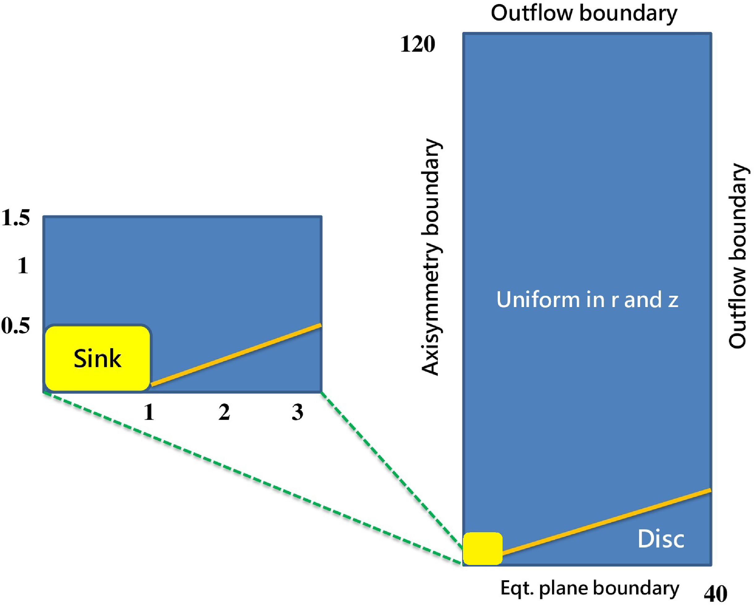
Figure 1. Schematic representation of the computational domain covering purely uniform spacing in radial and vertical directions. A zoom in on the bottom left corner of the grid is also shown to illustrate the sink, which is treated as an internal boundary. See the text for details.
We apply boundary conditions identical to those previously used in (Rezgui et al. Reference Rezgui, Marzougui, Woodring, Svoboda and Lili2019, Reference Rezgui, Marzougui, Lili, Preiner and Ceccobello2022). This maintains axial symmetry on the rotation axis and equatorial symmetry for the disc midplane. To the ghost cells at the upper r and z boundaries, we employ an outflow boundary condition (zero gradient). The sink zone, which is defined by the area where the central object is located (Fig. 1, yellow box), requires a specific treatment. Since the interaction between disc and central object is outside the purview of this investigation, we exclude this area (bottom-left corner) from the computational domain by cutting out several cells in r and z directions. Inside the sink, the equations are not evolved. We follow the same strategy as previous studies in literature, where the sink is treated as an internal boundary condition (Murphy, Ferreira, & Zanni Reference Murphy, Ferreira and Zanni2010; Tzeferacos et al. Reference Tzeferacos, Ferrari, Mignone, Zanni, Bodo and Massaglia2009, Reference Tzeferacos, Ferrari, Mignone, Zanni, Bodo and Massaglia2013). This latter has been discussed in our previous article Rezgui et al. (Reference Rezgui, Marzougui, Lili, Preiner and Ceccobello2022) (see Section 2.3). The most important point to consider is that we impose the non-positivity of the poloidal velocity in this area to ensure that no artificial outflows are permitted to leave the sink.
2.4. Simulation parameters
Our numerical calculations are governed by six nondimensional parameters for the physical quantities listed below:
-
The saturated thermal conduction parameter ${\unicode{x03D5}}_s$
-
The disc magnetisation
${\unicode{x03BC}} = B^2 \big /2P$
-
The sound-to-Keplerian speed ratio
${\unicode{x03B5}}= c_s \big /V_k$
-
The initial density contrast between disc and corona
${\unicode{x03B4}}$
-
The magnetic Prandtl number
$P_m$
-
The initial geometry of the magnetic field defined by the bending parameter m


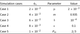
To investigate the thermal conduction contribution in the angular momentum transport and energy budget of the disc–jet system, we carried out five cases of numerical simulations based on the variation of the saturation parameter ${\unicode{x03D5}}_s$
. We adopt the same range values (Table 1, section on the left) of this parameter used in Rezgui et al. (Reference Rezgui, Marzougui, Woodring, Svoboda and Lili2019) and (Reference Rezgui, Marzougui, Lili, Preiner and Ceccobello2022). We point out that this range of values is close to those used in the studies of the advection-dominated accretion flows (ADAF systems) (Shadmehri Reference Shadmehri2008; Abbassi, Ghanbari, & Najjar Reference Abbassi, Ghanbari and Najjar2008; Ghanbari, Abbassi, & Ghasemnezhad Reference Ghanbari, Abbassi and Ghasemnezhad2009; Faghei Reference Faghei2012). In addition, we have shown in Rezgui et al. (Reference Rezgui, Marzougui, Lili, Preiner and Ceccobello2022) that it can be applied to YSOs such as the HH jets (Reipurth et al. Reference Reipurth, Davis, Bally, Raga, Bowler, Geballe, Aspin and Chiang2019; Ahmane et al. Reference Ahmane, Mignone, Zanni, Massaglia and Bouldjderi2020). We also show in Table 1 (section on the right) the values of the other five parameters that we kept constant in all our calculations.
${\unicode{x03D5}}_s$
. We adopt the same range values (Table 1, section on the left) of this parameter used in Rezgui et al. (Reference Rezgui, Marzougui, Woodring, Svoboda and Lili2019) and (Reference Rezgui, Marzougui, Lili, Preiner and Ceccobello2022). We point out that this range of values is close to those used in the studies of the advection-dominated accretion flows (ADAF systems) (Shadmehri Reference Shadmehri2008; Abbassi, Ghanbari, & Najjar Reference Abbassi, Ghanbari and Najjar2008; Ghanbari, Abbassi, & Ghasemnezhad Reference Ghanbari, Abbassi and Ghasemnezhad2009; Faghei Reference Faghei2012). In addition, we have shown in Rezgui et al. (Reference Rezgui, Marzougui, Lili, Preiner and Ceccobello2022) that it can be applied to YSOs such as the HH jets (Reipurth et al. Reference Reipurth, Davis, Bally, Raga, Bowler, Geballe, Aspin and Chiang2019; Ahmane et al. Reference Ahmane, Mignone, Zanni, Massaglia and Bouldjderi2020). We also show in Table 1 (section on the right) the values of the other five parameters that we kept constant in all our calculations.
Table 1. Range values of ${\unicode{x03D5}}_s$
(section on the left) and Input Parameters (section on the right).
${\unicode{x03D5}}_s$
(section on the left) and Input Parameters (section on the right).
We ran the code for advanced time steps. In fact, the simulations of cases 1 and 2 are performed up to $t = 700$
which indicates that the disc has completed 112 periods of rotation at its inner radius. While the final time step of the simulations of cases 3–5 is marked by
$t = 700$
which indicates that the disc has completed 112 periods of rotation at its inner radius. While the final time step of the simulations of cases 3–5 is marked by $t = 200$
roughly translated into 32 periods of rotation at the same disc radius. We have shown in our previous articles (Rezgui et al. Reference Rezgui, Marzougui, Woodring, Svoboda and Lili2019, Reference Rezgui, Marzougui, Lili, Preiner and Ceccobello2022) that the time
$t = 200$
roughly translated into 32 periods of rotation at the same disc radius. We have shown in our previous articles (Rezgui et al. Reference Rezgui, Marzougui, Woodring, Svoboda and Lili2019, Reference Rezgui, Marzougui, Lili, Preiner and Ceccobello2022) that the time $t = 200$
is sufficient to study the evolution of the disc–jet system, emphasising that the outflow was efficiently accelerated and reached the fast magnetosonic surface.
$t = 200$
is sufficient to study the evolution of the disc–jet system, emphasising that the outflow was efficiently accelerated and reached the fast magnetosonic surface.
3. Accretion–ejection simulations
In this section, we aim first to investigate the thermal conduction effects on the transport of the angular momentum from the accretion disc to the jet. We will then elucidate in-depth analysis the contribution of this physical ingredient in the energy balance of the disc–jet system.
3.1. Transport of angular momentum
The prevailing notion is that for successful jet formation, the magnetic torque must change its sign at the disc surface. This indicates that the predominant involvement in transferring angular momentum lies with the induced toroidal magnetic field component. As a result, the accretion flow is enabled inside the disc. Subsequently, the centrifugal force accelerates the material outward into the surrounding medium, where the jet extracts a portion of the angular momentum and energy from the disc.
We explore the angular momentum transport by means of its fluxes through the same control volume used to quantify the accretion and ejection rates. Following previous works (Zanni et al. Reference Zanni, Ferrari, Rosner, Bodo and Massaglia2007; Murphy, Ferreira, & Zanni Reference Murphy, Ferreira and Zanni2010, Tzeferacos et al. Reference Tzeferacos, Ferrari, Mignone, Zanni, Bodo and Massaglia2009, Reference Tzeferacos, Ferrari, Mignone, Zanni, Bodo and Massaglia2013), the integration domain (Fig. 2) is considered as a disc sector delimited by two surfaces $S_{in}$
and
$S_{in}$
and $S_{out}$
normal to the equatorial plane and identified at
$S_{out}$
normal to the equatorial plane and identified at $r_{in}$
and
$r_{in}$
and $r_{out}$
respectively. On top of the disc, we define an inclined surface, denoted
$r_{out}$
respectively. On top of the disc, we define an inclined surface, denoted $S_c$
through which the material escapes outwardly. Following Murphy, Ferreira, & Zanni (Reference Murphy, Ferreira and Zanni2010), we used
$S_c$
through which the material escapes outwardly. Following Murphy, Ferreira, & Zanni (Reference Murphy, Ferreira and Zanni2010), we used $r_{in} = 1.4$
and
$r_{in} = 1.4$
and $r_{out} = 5$
for calculation.
$r_{out} = 5$
for calculation.
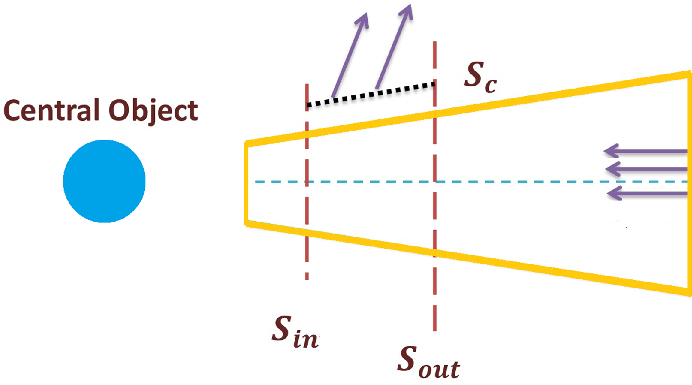
Figure 2. Schematic representation of the control volume used to compute the fluxes of the angular momentum and energy transport.
The accretion angular momentum flux is defined as $\dot{J}_{acc} = \dot{J}_{acc,kin} + \dot{J}_{acc,mag}$
where
$\dot{J}_{acc} = \dot{J}_{acc,kin} + \dot{J}_{acc,mag}$
where
 \begin{equation} \dot{J}_{acc,kin} = \int_{S_{in}} r_{in} {\unicode{x03C1}} U_{\unicode{x03D5}} \boldsymbol{U} \cdot dS - \int_{S_{out}} r_{out} {\unicode{x03C1}} U_{\unicode{x03D5}} \boldsymbol{U} \cdot dS\end{equation}
and
 \begin{equation} \dot{J}_{acc,mag} = \int_{S_{in}} r_{in} B_{\unicode{x03D5}} \boldsymbol{B} \cdot dS - \int_{S_{out}} r_{out} B_{\unicode{x03D5}} \boldsymbol{B} \cdot dS\end{equation}
The kinetic part $\dot{J}_{acc,kin}$
determines the flux of angular momentum inside the integration domain resulting from the inflow motion, while the magnetic part
$\dot{J}_{acc,kin}$
determines the flux of angular momentum inside the integration domain resulting from the inflow motion, while the magnetic part $\dot{J}_{acc,mag}$
defines the magnetic torque responsible for the radial transport of angular momentum inside the accretion disc.
$\dot{J}_{acc,mag}$
defines the magnetic torque responsible for the radial transport of angular momentum inside the accretion disc.
The angular momentum balance can be written as follows (Tzeferacos et al. Reference Tzeferacos, Ferrari, Mignone, Zanni, Bodo and Massaglia2013):
 \begin{equation} \dot{J}_{acc} = 2 \dot{J}_{jet} + \dot{J}_{visc}, \end{equation}
which shows that the angular momentum flux due to inflow is driven by the jet torque $\dot{J}_{jet}$
, defined as the torque exerted on the disc by the jet, or the viscous torque
$\dot{J}_{jet}$
, defined as the torque exerted on the disc by the jet, or the viscous torque $\dot{J}_{visc}$
which is due to viscous stresses. The ejection torque is also the sum of two parts:
$\dot{J}_{visc}$
which is due to viscous stresses. The ejection torque is also the sum of two parts: $\dot{J}_{jet} = \dot{J}_{jet,kin} + \dot{J}_{jet,mag}$
where
$\dot{J}_{jet} = \dot{J}_{jet,kin} + \dot{J}_{jet,mag}$
where
 \begin{equation} \dot{J}_{jet,kin} = \int_{S_c} r {\unicode{x03C1}} U_{\unicode{x03D5}} \boldsymbol{U} \cdot dS\end{equation}
and
 \begin{equation} \dot{J}_{jet,mag} = \int_{S_c} r B_{\unicode{x03D5}} \boldsymbol{B} \cdot dS\end{equation}
The viscous torque is defined as:
 \begin{equation} \dot{J}_{visc} = \int_{S_{in}} r \Pi \cdot dS - \int_{S_{out}} r \Pi \cdot dS\end{equation}
where $ \Pi$
is the viscous stress tensor introduced in equation (5).
$ \Pi$
is the viscous stress tensor introduced in equation (5).
We start by investigating the angular momentum transport inside the disc. We aim to shed light on the magnetic and kinetic contributions to the total accretion angular momentum. Fig. 3 shows the time evolution of the ratios $\dot{J}_{acc,kin} \big / \dot{J}_{acc}$
and
$\dot{J}_{acc,kin} \big / \dot{J}_{acc}$
and $\dot{J}_{acc,mag} \big / \dot{J}_{acc}$
for all cases of simulations until time step
$\dot{J}_{acc,mag} \big / \dot{J}_{acc}$
for all cases of simulations until time step $t=200$
. The conspicuous finding to emerge from this figure is that the kinetic torque represents the major contribution to
$t=200$
. The conspicuous finding to emerge from this figure is that the kinetic torque represents the major contribution to $\dot{J}_{acc}$
while the magnetic part represents a very small contribution to the total accretion angular momentum. We recorded, for example, that the kinetic and magnetic contributions to the total accretion angular momentum of case 1 at
$\dot{J}_{acc}$
while the magnetic part represents a very small contribution to the total accretion angular momentum. We recorded, for example, that the kinetic and magnetic contributions to the total accretion angular momentum of case 1 at $t=200$
are approximately 99% and 1%, respectively. These findings are consistent with previous works in the literature (Zanni et al. Reference Zanni, Ferrari, Rosner, Bodo and Massaglia2007; Tzeferacos et al. Reference Tzeferacos, Ferrari, Mignone, Zanni, Bodo and Massaglia2009).
$t=200$
are approximately 99% and 1%, respectively. These findings are consistent with previous works in the literature (Zanni et al. Reference Zanni, Ferrari, Rosner, Bodo and Massaglia2007; Tzeferacos et al. Reference Tzeferacos, Ferrari, Mignone, Zanni, Bodo and Massaglia2009).
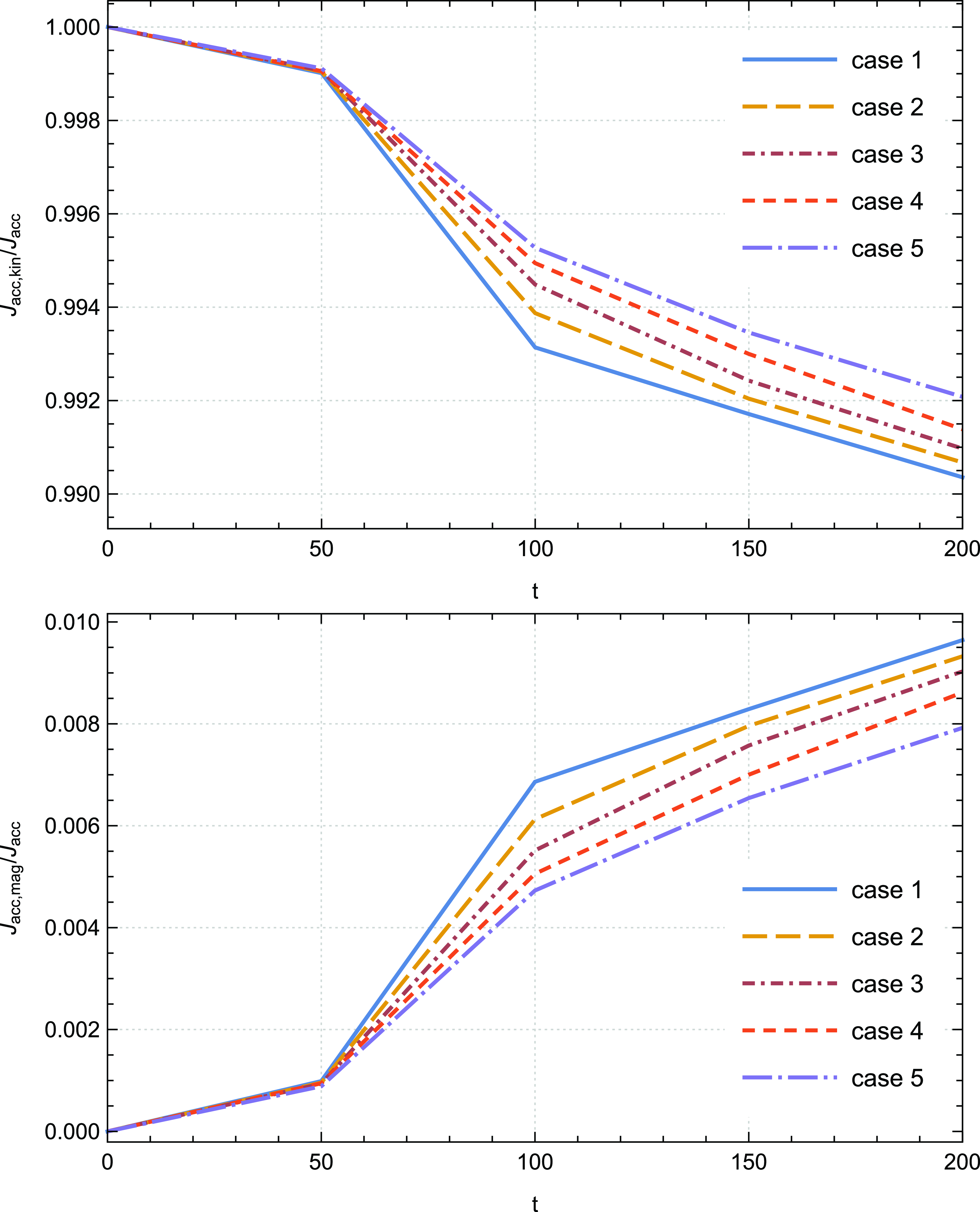
Figure 3. Time evolutions of the ratios $\dot{J}_{acc,kin}\big /\dot{J}_{acc}$
(top panel) and
$\dot{J}_{acc,kin}\big /\dot{J}_{acc}$
(top panel) and $\dot{J}_{acc,mag}\big /\dot{J}_{acc}$
(bottom panel) for the cases 1–5; case 1 (
$\dot{J}_{acc,mag}\big /\dot{J}_{acc}$
(bottom panel) for the cases 1–5; case 1 ( ${\unicode{x03D5}}_s= 0.002$
), case 2 (
${\unicode{x03D5}}_s= 0.002$
), case 2 ( ${\unicode{x03D5}}_s= 0.004$
), case 3 (
${\unicode{x03D5}}_s= 0.004$
), case 3 ( ${\unicode{x03D5}}_s= 0.006$
), case 4 (
${\unicode{x03D5}}_s= 0.006$
), case 4 ( ${\unicode{x03D5}}_s= 0.008$
), case 5 (
${\unicode{x03D5}}_s= 0.008$
), case 5 ( ${\unicode{x03D5}}_s= 0.01$
).
${\unicode{x03D5}}_s= 0.01$
).
Moreover, we find lower values of $\dot{J}_{acc,mag}\big /\dot{J}_{acc}$
than those recorded in these cited papers, which confirms that the magnetic torque acts to reduce the angular momentum. We also find that the ratio
$\dot{J}_{acc,mag}\big /\dot{J}_{acc}$
than those recorded in these cited papers, which confirms that the magnetic torque acts to reduce the angular momentum. We also find that the ratio $\dot{J}_{acc,mag}\big /\dot{J}_{acc,kin}$
does not exceed
$\dot{J}_{acc,mag}\big /\dot{J}_{acc,kin}$
does not exceed $2 \% $
for all our simulations, which is lower than that previously revealed in Zanni et al. (Reference Zanni, Ferrari, Rosner, Bodo and Massaglia2007) (about
$2 \% $
for all our simulations, which is lower than that previously revealed in Zanni et al. (Reference Zanni, Ferrari, Rosner, Bodo and Massaglia2007) (about $10 \%$
). Inside the disc, the kinetic torque plays therefore the important role in the angular momentum transport.
$10 \%$
). Inside the disc, the kinetic torque plays therefore the important role in the angular momentum transport.
Interestingly, increasing the saturation parameter ${\unicode{x03D5}}_s$
leads to an increase in the amplitude of the ratio
${\unicode{x03D5}}_s$
leads to an increase in the amplitude of the ratio $\dot{J}_{acc,kin}\big /\dot{J}_{acc}$
and to a decrease in the ratio
$\dot{J}_{acc,kin}\big /\dot{J}_{acc}$
and to a decrease in the ratio $\dot{J}_{acc,mag}\big /\dot{J}_{acc}$
until the time step
$\dot{J}_{acc,mag}\big /\dot{J}_{acc}$
until the time step $t=200$
. Thermal conduction acts then to further promote accretion, which makes the inner area of the disc denser, proving the presence of a sufficient material that can be ejected outward. This effect is reversed at advanced times of the simulations where the jet moves far enough from the disc. We observe in Fig. 4 particularly from
$t=200$
. Thermal conduction acts then to further promote accretion, which makes the inner area of the disc denser, proving the presence of a sufficient material that can be ejected outward. This effect is reversed at advanced times of the simulations where the jet moves far enough from the disc. We observe in Fig. 4 particularly from $t= 500$
a decrease in the amplitude of
$t= 500$
a decrease in the amplitude of $\dot{J}_{acc,kin}\big /\dot{J}_{acc}$
in presence of thermal conduction. This observation aligns with our prior work (Rezgui et al. Reference Rezgui, Marzougui, Woodring, Svoboda and Lili2019) where we showed that thermal conduction acts, at
$\dot{J}_{acc,kin}\big /\dot{J}_{acc}$
in presence of thermal conduction. This observation aligns with our prior work (Rezgui et al. Reference Rezgui, Marzougui, Woodring, Svoboda and Lili2019) where we showed that thermal conduction acts, at $t=500$
, to decelerate the disc’s angular velocity
$t=500$
, to decelerate the disc’s angular velocity $U_{\unicode{x03D5}}$
(note that the kinetic torque profile depends on
$U_{\unicode{x03D5}}$
(note that the kinetic torque profile depends on $U_{\unicode{x03D5}}$
). This has been attributed to the dominance of gravity over centrifugal force, allowing the inflow towards the central object. It is also evident to notice the plateau reached by the quantity
$U_{\unicode{x03D5}}$
). This has been attributed to the dominance of gravity over centrifugal force, allowing the inflow towards the central object. It is also evident to notice the plateau reached by the quantity $\dot{J}_{acc,kin}\big /\dot{J}_{acc}$
identified for the case 2 from
$\dot{J}_{acc,kin}\big /\dot{J}_{acc}$
identified for the case 2 from $t = 400$
until the final time step of our calculations. This finding pleads in favour of the quasi-stationarity of the solutions in presence of thermal conduction.
$t = 400$
until the final time step of our calculations. This finding pleads in favour of the quasi-stationarity of the solutions in presence of thermal conduction.
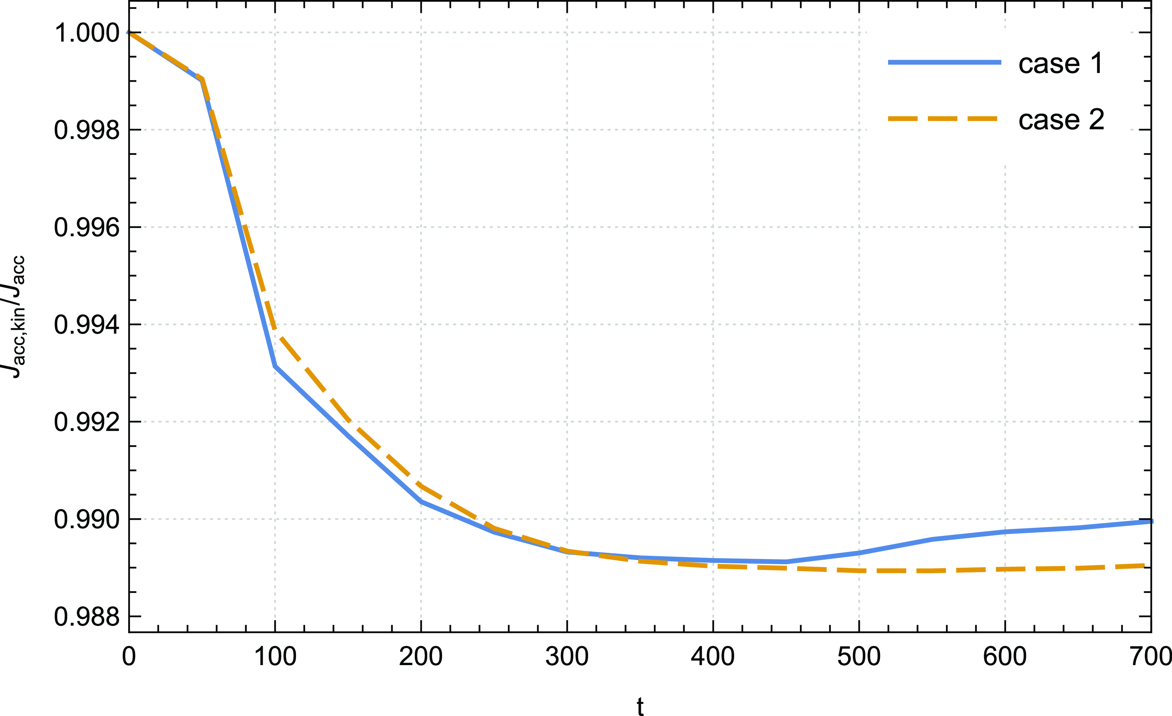
Figure 4. Time evolution of the ratio $\dot{J}_{acc,kin}\big /\dot{J}_{acc}$
of case 1 (
$\dot{J}_{acc,kin}\big /\dot{J}_{acc}$
of case 1 ( ${\unicode{x03D5}}_s= 0.002$
) and case 2 (
${\unicode{x03D5}}_s= 0.002$
) and case 2 ( ${\unicode{x03D5}}_s= 0.004$
).
${\unicode{x03D5}}_s= 0.004$
).
It is commonly accepted that the differential motion between the disc layers leads to the transfer of angular momentum from the inner parts of the disc to the outer parts, since the viscosity causes the adjacent layers of fluid in the disc to move at different speeds. Irrespective of the specific mechanism accountable for viscosity in accretion discs, previous studies (Murphy, Ferreira, & Zanni Reference Murphy, Ferreira and Zanni2010; Tzeferacos et al. Reference Tzeferacos, Ferrari, Mignone, Zanni, Bodo and Massaglia2013) have indicated that this process does not significantly affect the evolution of the disc-jet system. However, we will briefly examine the impact of thermal conduction on the temporal evolution of the viscous torque $\dot{J}_{visc}$
.
$\dot{J}_{visc}$
.
Fig. 5 depicts its profile for all our cases of simulations. After a few oscillations at the initial time steps, we observe that the viscous torque gradually decreases over time, and it is obvious to notice that it converges towards very low values. This behaviour indicates that its role in the angular momentum transport becomes less important as the accretion–ejection structure becomes fully established. Increasing the saturation parameter ${\unicode{x03D5}}_s$
leads to an increase in the amplitude of the viscous torque. This can be explained by the fact that the gas in the inner regions experiences a torque that causes it to lose more angular momentum and moves inward, while the gas in the outer regions experiences a torque that causes it to gain more angular momentum and moves outwards. Hence, within the disc’s inner region, gravity prevails over centrifugal force due to increased braking of its rings. This mechanism enables the accretion of additional material onto the central object. Nevertheless, the thermal conduction effect on the time evolution of
${\unicode{x03D5}}_s$
leads to an increase in the amplitude of the viscous torque. This can be explained by the fact that the gas in the inner regions experiences a torque that causes it to lose more angular momentum and moves inward, while the gas in the outer regions experiences a torque that causes it to gain more angular momentum and moves outwards. Hence, within the disc’s inner region, gravity prevails over centrifugal force due to increased braking of its rings. This mechanism enables the accretion of additional material onto the central object. Nevertheless, the thermal conduction effect on the time evolution of $\dot{J}_{visc}$
is not substantial at advanced time steps of our calculations, as previously mentioned.
$\dot{J}_{visc}$
is not substantial at advanced time steps of our calculations, as previously mentioned.
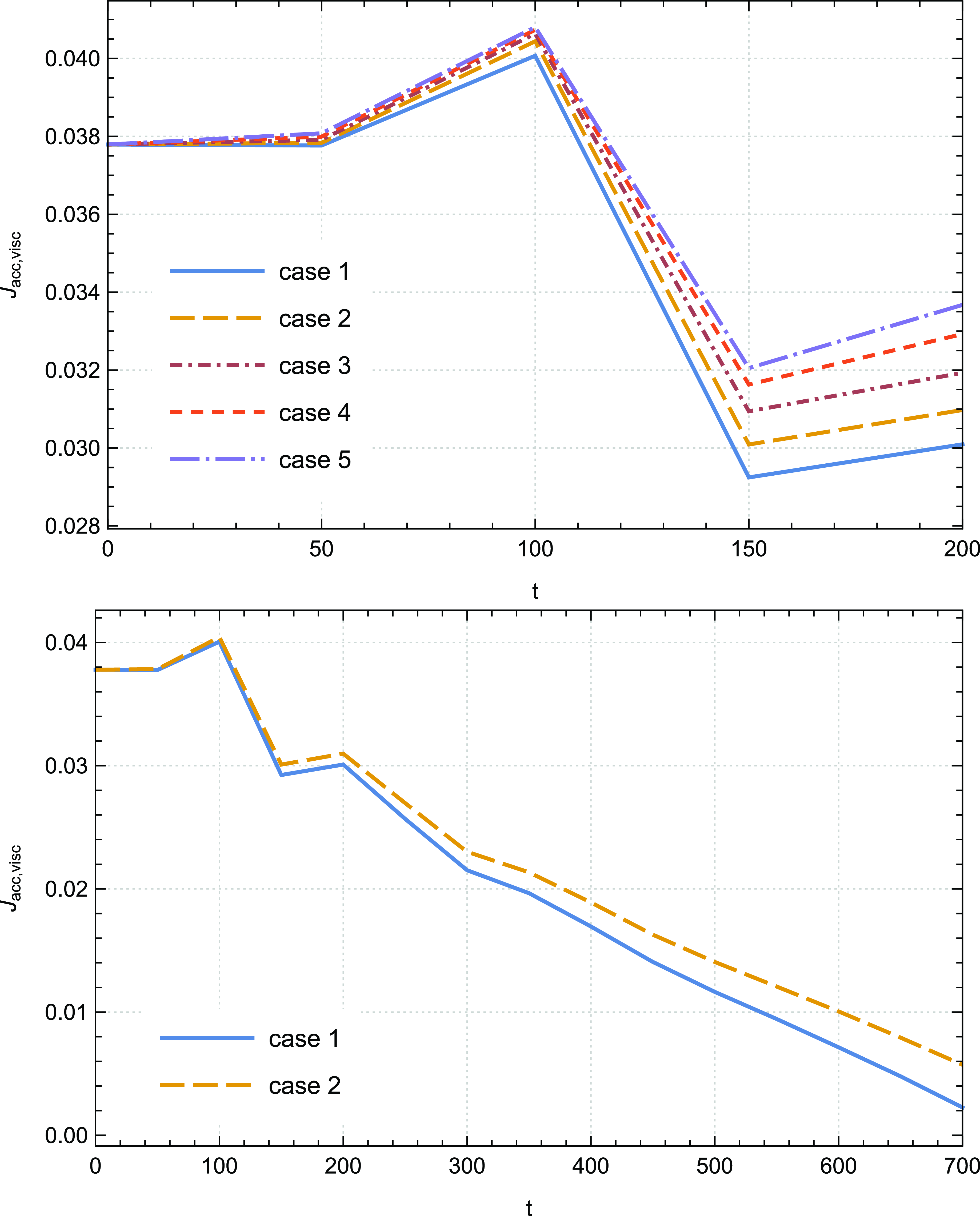
Figure 5. Temporal evolution of the viscous torque $\dot{J}_{visc}$
for cases 1–5 up to
$\dot{J}_{visc}$
for cases 1–5 up to $t=200$
(top panel) and for cases 1–2 up to
$t=200$
(top panel) and for cases 1–2 up to $t=700$
(bottom panel); case 1 (
$t=700$
(bottom panel); case 1 ( ${\unicode{x03D5}}_s= 0.002$
), case 2 (
${\unicode{x03D5}}_s= 0.002$
), case 2 ( ${\unicode{x03D5}}_s= 0.004$
), case 3 (
${\unicode{x03D5}}_s= 0.004$
), case 3 ( ${\unicode{x03D5}}_s= 0.006$
), case 4 (
${\unicode{x03D5}}_s= 0.006$
), case 4 ( ${\unicode{x03D5}}_s= 0.008$
), case 5 (
${\unicode{x03D5}}_s= 0.008$
), case 5 ( ${\unicode{x03D5}}_s= 0.01$
).
${\unicode{x03D5}}_s= 0.01$
).
Within the same context, we also place a similar emphasis on examining the impact of thermal conduction on the ejection torque, which pertains to the torque exerted by the outflow on the disc. The relative contributions of the magnetic and kinetic parts to the total ejection angular momentum $\dot{J}_{jet}$
differ from those within the disc. In fact, we show in Fig. 6 the evolution in time of the ratios
$\dot{J}_{jet}$
differ from those within the disc. In fact, we show in Fig. 6 the evolution in time of the ratios $\dot{J}_{jet,mag} \big /\dot{J}_{jet}$
and
$\dot{J}_{jet,mag} \big /\dot{J}_{jet}$
and $\dot{J}_{jet,kin} \big /\dot{J}_{jet}$
respectively, for cases 1–2 until the final time step of our simulations.
$\dot{J}_{jet,kin} \big /\dot{J}_{jet}$
respectively, for cases 1–2 until the final time step of our simulations.
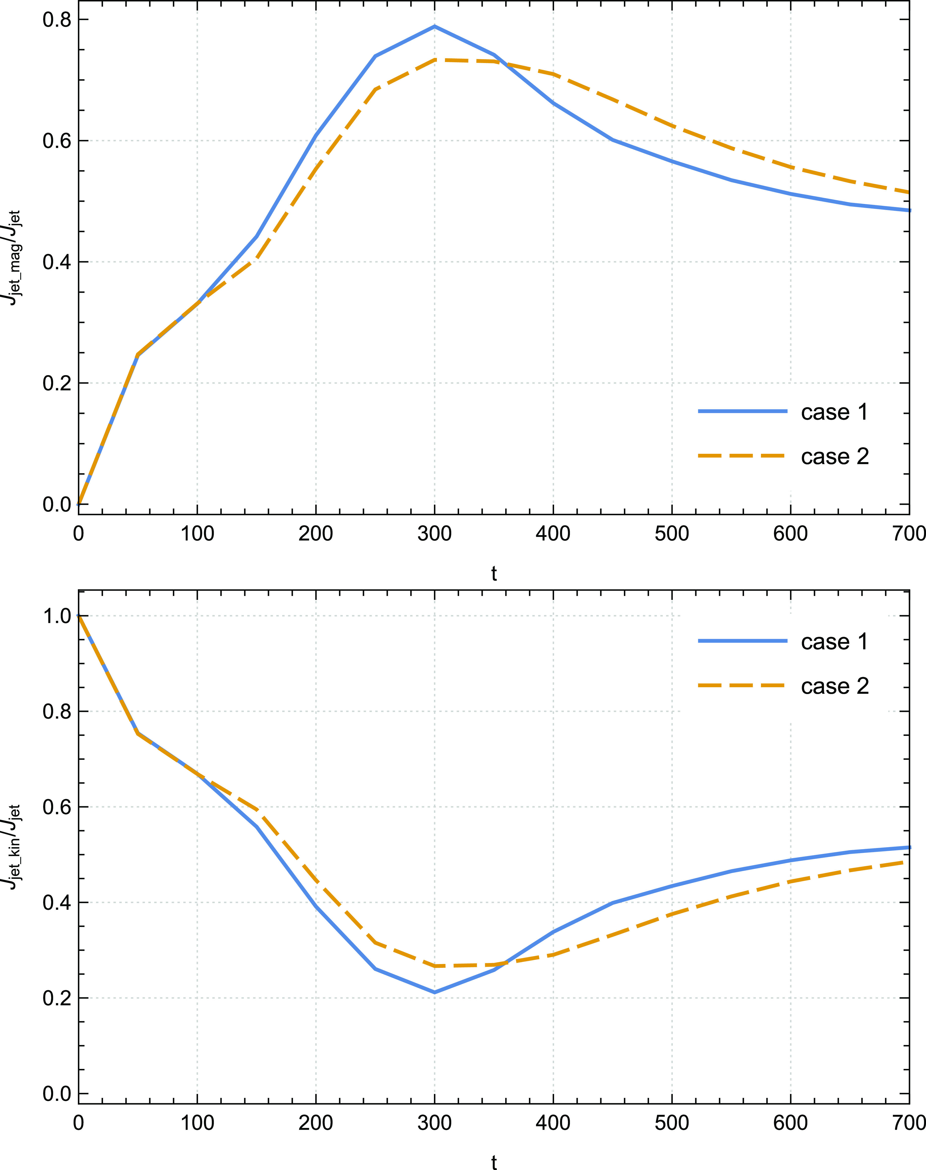
Figure 6. Temporal evolution of the ratios $\dot{J}_{jet,mag} \big /\dot{J}_{jet}$
(top panel) and
$\dot{J}_{jet,mag} \big /\dot{J}_{jet}$
(top panel) and $\dot{J}_{jet,kin} \big /\dot{J}_{jet}$
(bottom panel) for cases 1–2 up to
$\dot{J}_{jet,kin} \big /\dot{J}_{jet}$
(bottom panel) for cases 1–2 up to $t=700$
; case 1 (
$t=700$
; case 1 ( ${\unicode{x03D5}}_s= 0.002$
), case 2 (
${\unicode{x03D5}}_s= 0.002$
), case 2 ( ${\unicode{x03D5}}_s= 0.004$
).
${\unicode{x03D5}}_s= 0.004$
).
One of the essential findings from the first sight of these curves is that the main contribution to the total ejection angular momentum is attributed to the magnetic part, in contrast to what is revealed inside the disc. This feature becomes prominent starting at time step $t=200$
where
$t=200$
where $\dot{J}_{jet,mag}$
represents approximately 60–80% of the total ejection angular momentum. This result is in concordance with the previous simulations conducted by Tzeferacos et al. (Reference Tzeferacos, Ferrari, Mignone, Zanni, Bodo and Massaglia2009). Even more crucial is that at advanced time steps, particularly from
$\dot{J}_{jet,mag}$
represents approximately 60–80% of the total ejection angular momentum. This result is in concordance with the previous simulations conducted by Tzeferacos et al. (Reference Tzeferacos, Ferrari, Mignone, Zanni, Bodo and Massaglia2009). Even more crucial is that at advanced time steps, particularly from $t=350$
, thermal conduction plays an essential role by enhancing the influence of the magnetic component
$t=350$
, thermal conduction plays an essential role by enhancing the influence of the magnetic component $\dot{J}_{jet,mag} \big /\dot{J}_{jet}$
while decreasing the impact of the kinetic component
$\dot{J}_{jet,mag} \big /\dot{J}_{jet}$
while decreasing the impact of the kinetic component $\dot{J}_{jet,kin} \big /\dot{J}_{jet}$
.
$\dot{J}_{jet,kin} \big /\dot{J}_{jet}$
.
In order to give more insight about this behaviour, it is therefore essential to hearken back to the thermal conduction role in the magnetocentrifugal mechanism (Blandford & Payne Reference Blandford and Payne1982) discussed in our previous paper Rezgui et al. (Reference Rezgui, Marzougui, Lili, Preiner and Ceccobello2022) where the investigation of the vertical dependence of the ratio $\vert B_{\unicode{x03D5}}\vert \big /B_p$
revealed that the toroidal magnetic acceleration becomes stronger in presence of thermal conduction which suggests that the magnetic field has a complete control over the ejected plasma and compels it to corotate with the field lines. We emphasised that the magnetic energy stored in the toroidal component of the Lorentz force at the disc surface propels the plasma along the magnetic field lines. This finding serves as a compelling argument supporting the notion that thermal conduction gives more weight to the contribution of the magnetic component
$\vert B_{\unicode{x03D5}}\vert \big /B_p$
revealed that the toroidal magnetic acceleration becomes stronger in presence of thermal conduction which suggests that the magnetic field has a complete control over the ejected plasma and compels it to corotate with the field lines. We emphasised that the magnetic energy stored in the toroidal component of the Lorentz force at the disc surface propels the plasma along the magnetic field lines. This finding serves as a compelling argument supporting the notion that thermal conduction gives more weight to the contribution of the magnetic component $\dot{J}_{jet,mag}$
to the total ejection angular momentum.
$\dot{J}_{jet,mag}$
to the total ejection angular momentum.
In the same vein, it is valuable to assess the effectiveness of the magnetocentrifugal mechanism by examining the ratio between the magnetic $\dot{J}_{jet,mag}$
and the kinetic
$\dot{J}_{jet,mag}$
and the kinetic $\dot{J}_{jet,kin}$
torque. Fig. 7 provides a visualisation of the temporal evolution of this ratio for cases 1 and 2. As the jet propagates along the axis of rotation of the disc, we observe a noticeable increase in this ratio. Beyond a certain time step, specifically
$\dot{J}_{jet,kin}$
torque. Fig. 7 provides a visualisation of the temporal evolution of this ratio for cases 1 and 2. As the jet propagates along the axis of rotation of the disc, we observe a noticeable increase in this ratio. Beyond a certain time step, specifically $t = 200$
, the magnetic component dominates the kinetic component, with the ratio exceeding unity. In case 1 of our simulations, we identify a peak at
$t = 200$
, the magnetic component dominates the kinetic component, with the ratio exceeding unity. In case 1 of our simulations, we identify a peak at $t=300$
where the magnetic torque
$t=300$
where the magnetic torque $\dot{J}_{jet,mag}$
is found to be
$\dot{J}_{jet,mag}$
is found to be $3.8$
times greater than the kinetic torque
$3.8$
times greater than the kinetic torque $\dot{J}_{jet,kin}$
. Concretely, we record an improvement of approximately
$\dot{J}_{jet,kin}$
. Concretely, we record an improvement of approximately $23.7\% $
in the integral of this ratio from
$23.7\% $
in the integral of this ratio from $t = 400$
up to the final time step of our runs in case 2 relative to case 1. A higher ratio signifies a larger amount of specific angular momentum accessible at the disc’s surface, resulting in an increase in centrifugal acceleration and, consequently, higher poloidal terminal speeds for the plasma.
$t = 400$
up to the final time step of our runs in case 2 relative to case 1. A higher ratio signifies a larger amount of specific angular momentum accessible at the disc’s surface, resulting in an increase in centrifugal acceleration and, consequently, higher poloidal terminal speeds for the plasma.
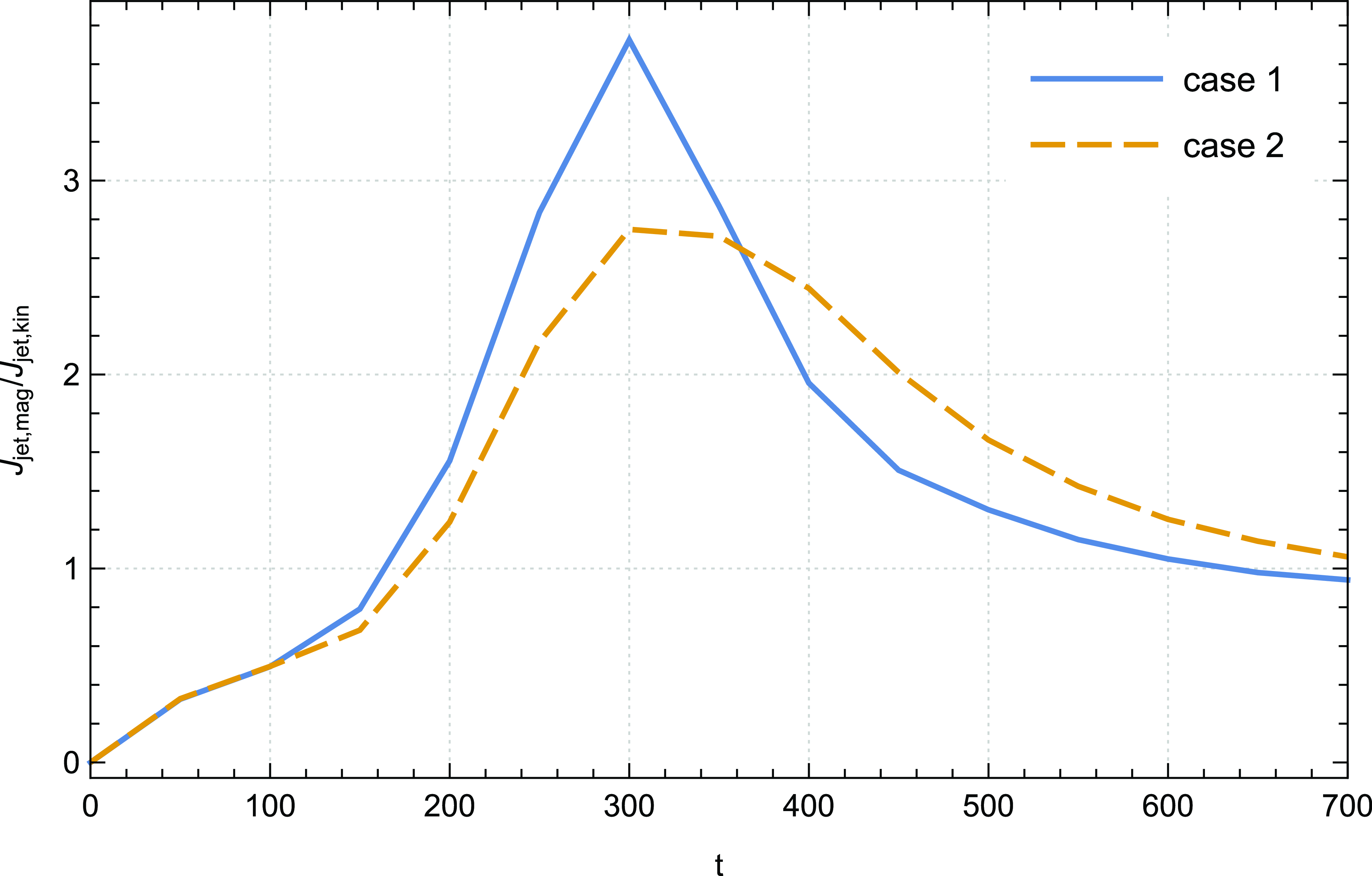
Figure 7. Time evolution of the ratio $\dot{J}_{jet,mag}\big /\dot{J}_{jet,kin}$
of case 1 (
$\dot{J}_{jet,mag}\big /\dot{J}_{jet,kin}$
of case 1 ( ${\unicode{x03D5}}_s= 0.002$
) and case 2 (
${\unicode{x03D5}}_s= 0.002$
) and case 2 ( ${\unicode{x03D5}}_s= 0.004$
).
${\unicode{x03D5}}_s= 0.004$
).
It presents compelling evidence and detailed support for the notion that the accretion–ejection structure is primarily influenced by the magnetic force, with the magnetic contribution becoming increasingly dominant over the kinetic contribution in the presence of thermal conduction at advanced time steps.
It is interesting to present a detailed illustration of the angular momentum distribution in the disc-jet system over time. To this end, we compute the angular momentum flux $\dot J= r {\unicode{x03C1}} U_{\unicode{x03D5}} \boldsymbol{U} - r B_{\unicode{x03D5}} \boldsymbol{B}$
for cylindrical coordinates within each cell of the computation grid. In Fig. 8, we show the log-magnitude of
$\dot J= r {\unicode{x03C1}} U_{\unicode{x03D5}} \boldsymbol{U} - r B_{\unicode{x03D5}} \boldsymbol{B}$
for cylindrical coordinates within each cell of the computation grid. In Fig. 8, we show the log-magnitude of $\dot J$
per cell sample of our reference case 1 across varying time steps. Notably, from the time step
$\dot J$
per cell sample of our reference case 1 across varying time steps. Notably, from the time step $t=50$
, our findings vividly demonstrate the establishment and evolution of the accretion-ejection structure within the system. The discernible variation in the magnitude of
$t=50$
, our findings vividly demonstrate the establishment and evolution of the accretion-ejection structure within the system. The discernible variation in the magnitude of $\dot J$
unequivocally indicates the extraction of angular momentum from the disc surface by the jet. Simultaneously, our observations highlight the concurrent accretion of matter towards the central object.
$\dot J$
unequivocally indicates the extraction of angular momentum from the disc surface by the jet. Simultaneously, our observations highlight the concurrent accretion of matter towards the central object.
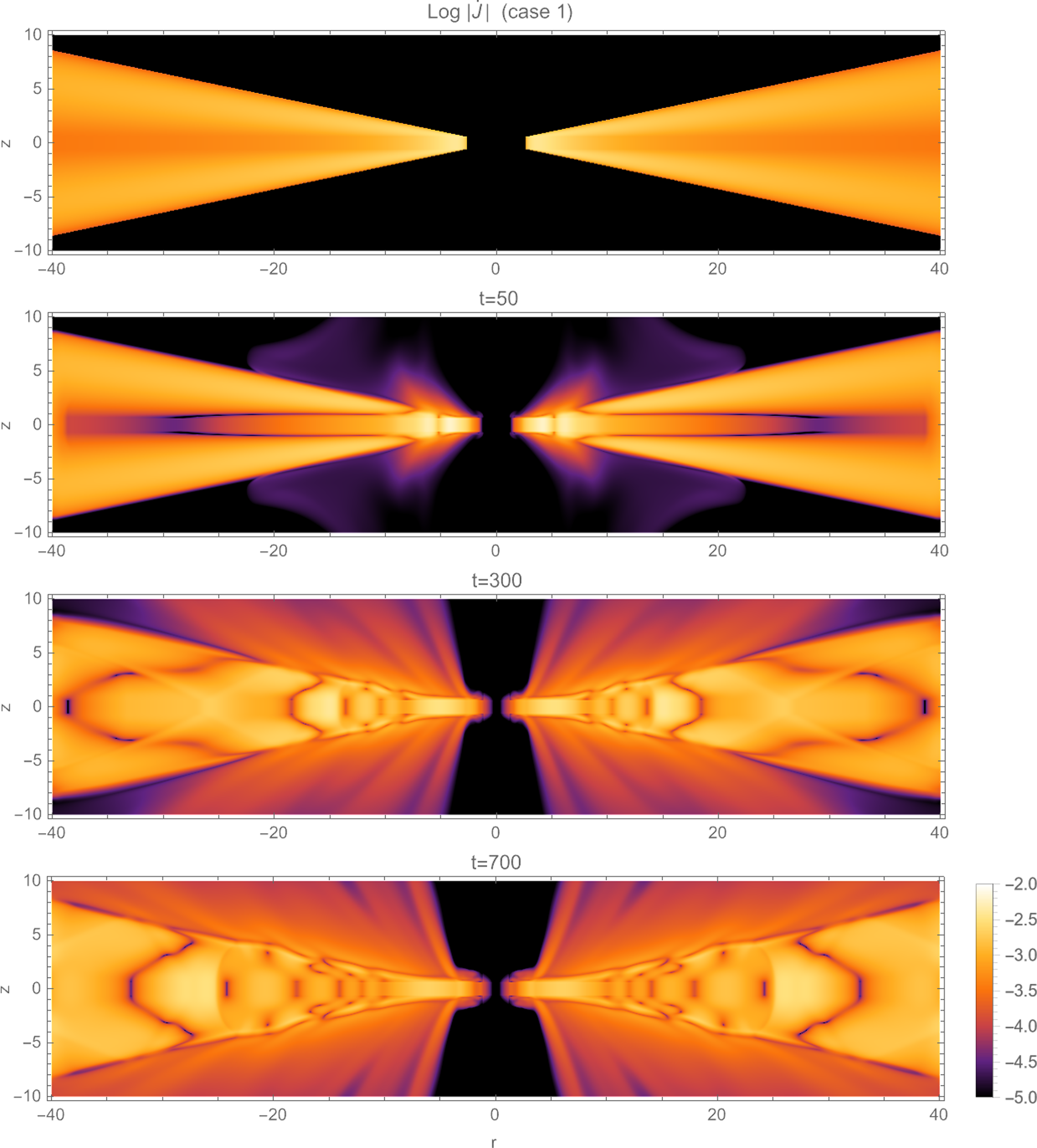
Figure 8. Log-magnitude distribution of the angular momentum flux $ \dot J= r {\unicode{x03C1}} U_{\unicode{x03D5}} \boldsymbol{U} - r B_{\unicode{x03D5}} \boldsymbol{B}$
in the disc–jet system of case 1 (
$ \dot J= r {\unicode{x03C1}} U_{\unicode{x03D5}} \boldsymbol{U} - r B_{\unicode{x03D5}} \boldsymbol{B}$
in the disc–jet system of case 1 ( ${\unicode{x03D5}}_s= 0.002$
) for dynamical time steps (from top to bottom):
${\unicode{x03D5}}_s= 0.002$
) for dynamical time steps (from top to bottom): $t = 0$
,
$t = 0$
, $t = 50$
,
$t = 50$
, $t = 300$
and
$t = 300$
and $t = 700$
.
$t = 700$
.
In Fig. 9, we extend our visualisation methodology to depict the temporal evolution of the log-magnitudes concerning the magnetic and kinetic constituents of the angular momentum flux within the intricate dynamics of the disc-jet system. Employing distinct monochromatic colour gradients (green for the kinetic component and blue for the magnetic component) in the first and second rows respectively, the third row of this illustration presents a compelling visual decomposition into these components, offering insights into their spatial coexistence. This comprehensive analysis corroborates our findings discussed above, emphasising the individual contributions of each component to the overall angular momentum.
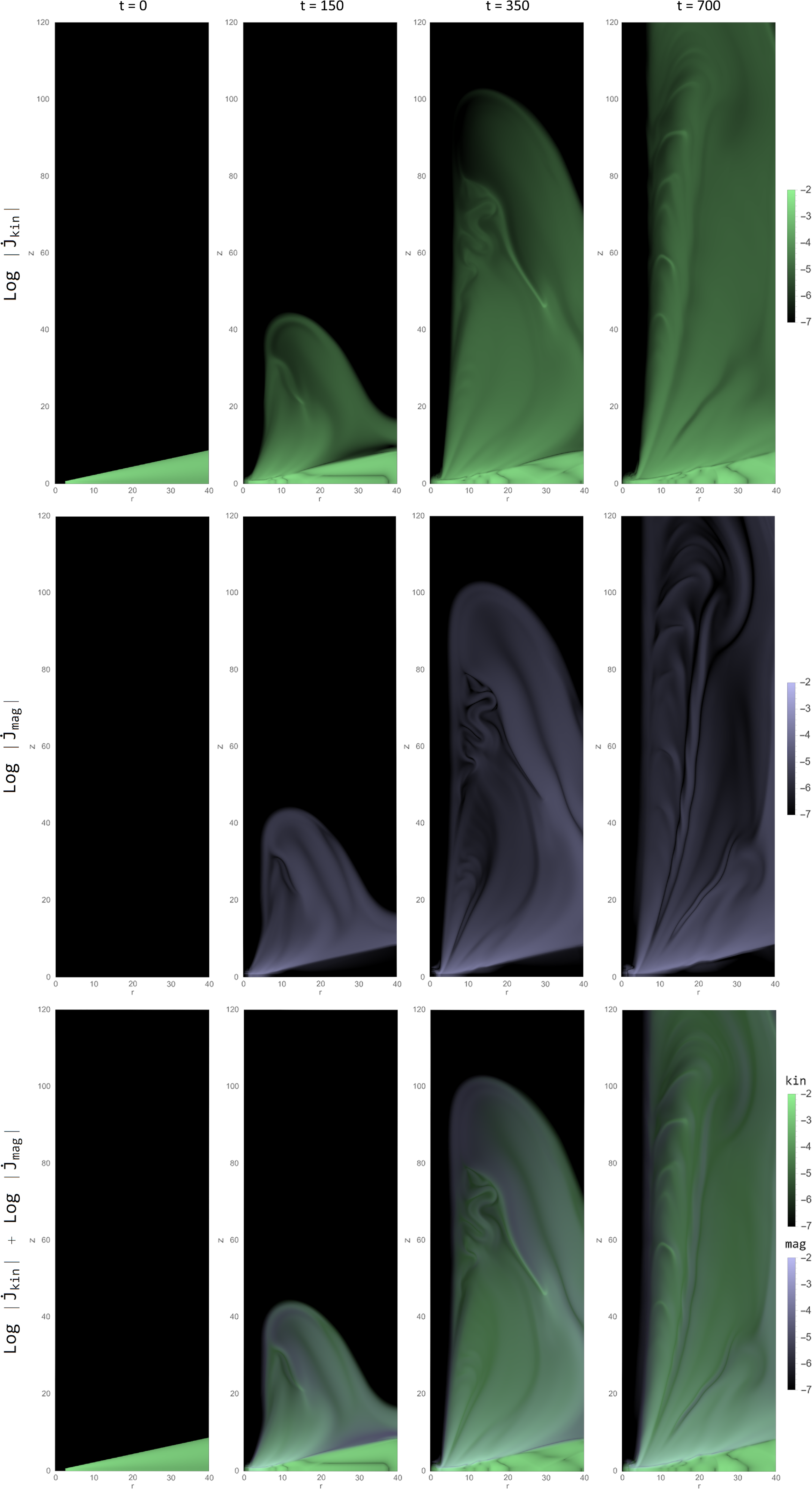
Figure 9. Time evolution of log-magnitude of the kinetic component log $\big \vert \dot{J}_{kin} \big \vert $
(top panel), log-magnitude of the magnetic component log
$\big \vert \dot{J}_{kin} \big \vert $
(top panel), log-magnitude of the magnetic component log $\big \vert \dot{J}_{mag} \big \vert $
(central panel), and visual overlay of the sum of two components: log
$\big \vert \dot{J}_{mag} \big \vert $
(central panel), and visual overlay of the sum of two components: log $ \big \vert \dot{J}_{kin} \big \vert$
+ log
$ \big \vert \dot{J}_{kin} \big \vert$
+ log $\big \vert \dot{J}_{mag} \big \vert$
(bottom panel) in the disc–jet system of case 1 (
$\big \vert \dot{J}_{mag} \big \vert$
(bottom panel) in the disc–jet system of case 1 ( ${\unicode{x03D5}}_s= 0.002$
).
${\unicode{x03D5}}_s= 0.002$
).
Notably, the magnetic component (illustrated in the second row) primarily exerts influence within the jet region, while the kinetic component (shown in the first row) exhibits relevance across the entire structure. The third row’s composite visualisation delineates the dominance of the kinetic component within the accretion disc and unveils the concurrent presence of both components within the jet, shedding light on their coexistence and respective roles within distinct regions of the system. This detailed depiction affords a deeper understanding of the nuanced interplay between magnetic and kinetic elements in shaping the angular momentum dynamics within the disc-jet paradigm.
3.2. Energy budget of the disc–jet system
Within this section, our examination focuses on the role of thermal conduction in the energetics of the disc–jet system. Similarly to the analysis of angular momentum transfer, we explore the energy fluxes through the control volume introduced in Fig. 2.
The theoretical global energy budget can be written as:
 \begin{equation} \dot{E}_{lib} = \dot{E}_{jet} + \dot{E}_{rad}\end{equation}
where $ \dot{E}_{lib} = \dot{E}_{acc} + \dot{E}_{visc} + \dot{E}_{cond}$
is the actual power that is liberated within the disc.
$ \dot{E}_{lib} = \dot{E}_{acc} + \dot{E}_{visc} + \dot{E}_{cond}$
is the actual power that is liberated within the disc. $\dot{E}_{acc}$
is the total accretion power (accretion energy flux) which is defined as the sum of the mechanical (gravitational and kinetic), magnetic and enthalpy energy fluxes which are expressed as follows:
$\dot{E}_{acc}$
is the total accretion power (accretion energy flux) which is defined as the sum of the mechanical (gravitational and kinetic), magnetic and enthalpy energy fluxes which are expressed as follows:
 \begin{equation} \dot{E}_{acc,grav} = \int_{S_{in}} \Phi_g {\unicode{x03C1}} \boldsymbol{U} \cdot dS - \int_{S_{out}} \Phi_g {\unicode{x03C1}} \boldsymbol{U} \cdot dS\end{equation}
 \begin{equation} \dot{E}_{acc,kin} = \int_{S_{in}} \frac{1}{2} U^2 {\unicode{x03C1}} \boldsymbol{U} \cdot dS - \int_{S_{out}} \frac{1}{2} U^2 {\unicode{x03C1}} \boldsymbol{U} \cdot dS\end{equation}
 \begin{equation} \dot{E}_{acc,mag} = \int_{S_{in}} \boldsymbol{E} \times \boldsymbol{B} \ \cdot dS - \int_{S_{out}} \boldsymbol{E} \times \boldsymbol{B} \cdot dS\end{equation}
 \begin{equation} \dot{E}_{acc,enth} = \int_{S_{in}} \frac{{\unicode{x03B3}}}{{\unicode{x03B3}}-1} P \boldsymbol{U} \cdot dS - \int_{S_{out}} \frac{{\unicode{x03B3}}}{{\unicode{x03B3}}-1} P \boldsymbol{U} \cdot dS\end{equation} $\dot{E}_{visc}$
is the flux of energy due to viscosity and defined as:
$\dot{E}_{visc}$
is the flux of energy due to viscosity and defined as:
 \begin{equation} \dot{E}_{visc} = \int_{S_{in}} {\boldsymbol{u}} \Pi \cdot dS - \int_{S_{out}} {\boldsymbol{u}} \Pi \cdot dS\end{equation} $\dot{E}_{cond}$
is the flux of energy due to thermal conduction and can be written as:
$\dot{E}_{cond}$
is the flux of energy due to thermal conduction and can be written as:
 \begin{equation} \dot{E}_{cond} = \int_{S_{in}} \nabla \cdot \boldsymbol{F}_c \cdot dS - \int_{S_{out}} \nabla \cdot \boldsymbol{F}_c \cdot dS\end{equation} $\dot{E}_{jet}$
is the jet power characterising the energy extracted by the outflow. It is calculated as the sum of all energy fluxes (mechanical, Poynting, and enthalpy) leaving the disc surface:
$\dot{E}_{jet}$
is the jet power characterising the energy extracted by the outflow. It is calculated as the sum of all energy fluxes (mechanical, Poynting, and enthalpy) leaving the disc surface:
 \begin{equation} \dot{E}_{jet} = \dot{E}_{jet,kin} + \dot{E}_{jet,grav} + \dot{E}_{jet,mag} + \dot{E}_{jet,enth}\end{equation}
where
 \begin{equation} \dot{E}_{jet,kin} = \int_{S_c} \frac{1}{2} U^2 {\unicode{x03C1}} \boldsymbol{U} \cdot dS\end{equation}
 \begin{equation} \dot{E}_{jet,grav} = \int_{S_c} \Phi_g {\unicode{x03C1}} \boldsymbol{U} \cdot dS\end{equation}
 \begin{equation} \dot{E}_{jet,mag} = \int_{S_c} \boldsymbol{E} \times \boldsymbol{B} \ \cdot dS\end{equation}
 \begin{equation} \dot{E}_{jet,enth} = \int_{S_c} \frac{{\unicode{x03B3}}}{{\unicode{x03B3}}-1} P \boldsymbol{U} \cdot dS\end{equation} $\dot{E}_{rad}$
represents the power released into heat by both Joule and viscous terms, which is eventually emitted as radiation from the surface of the disc. Following Murphy, Ferreira, & Zanni (Reference Murphy, Ferreira and Zanni2010) our calculation does not account for radiation. However, we ensure that the Joule and viscous heating effects are balanced by the cooling term
$\dot{E}_{rad}$
represents the power released into heat by both Joule and viscous terms, which is eventually emitted as radiation from the surface of the disc. Following Murphy, Ferreira, & Zanni (Reference Murphy, Ferreira and Zanni2010) our calculation does not account for radiation. However, we ensure that the Joule and viscous heating effects are balanced by the cooling term $\zeta_{cool}$
(equation (6)).
$\zeta_{cool}$
(equation (6)).
In the preceding section of this paper, we showed that the contribution of the viscous torque to the angular momentum transport within the disc is not significant. Therefore, we will not delve, as prior studies (Murphy, Ferreira, & Zanni Reference Murphy, Ferreira and Zanni2010; Tzeferacos et al. Reference Tzeferacos, Ferrari, Mignone, Zanni, Bodo and Massaglia2013), into an in-depth analysis of the effects of the viscous power on the energy balance of the disc-jet system. Instead, our primary focus will be on comparing the power generated by the jet with the power derived from accretion, as well as the energy flux associated with thermal conduction. By concentrating our efforts on these specific aspects, we aim to shed light on the intricate interplay between these sources of energy in the system under study.
We commence by elucidating how the existence of thermal conduction influences the total accretion power and then unravel the diverse contributions to $\dot{E}_{acc}$
. We show in Fig. 10 the time evolution of the total accretion power for the cases considered in this work. At initial time steps, a remarkable observation is the sudden surge in the amplitude of the accretion power, particularly from
$\dot{E}_{acc}$
. We show in Fig. 10 the time evolution of the total accretion power for the cases considered in this work. At initial time steps, a remarkable observation is the sudden surge in the amplitude of the accretion power, particularly from $t= 100$
, indicating the successful operation of the inflow mechanism, effectively delivering material to the disc. Subsequently, after a few fluctuations, particularly from
$t= 100$
, indicating the successful operation of the inflow mechanism, effectively delivering material to the disc. Subsequently, after a few fluctuations, particularly from $t = 300$
, an intriguing correlation emerges between the saturation parameter
$t = 300$
, an intriguing correlation emerges between the saturation parameter ${\unicode{x03D5}}_s$
and the accretion power. As the saturation parameter increases, so does the amplitude of the accretion power. Specifically, we record an improvement of approximately
${\unicode{x03D5}}_s$
and the accretion power. As the saturation parameter increases, so does the amplitude of the accretion power. Specifically, we record an improvement of approximately $2\% $
in the integral accretion power from
$2\% $
in the integral accretion power from $t=400$
up to the final time step of our calculations in case 2 relative to case 1. This relationship demonstrates the influence of thermal conduction within the system, as it enhances the energy content within the control volume and consequently, boosts the overall energy output. Notice that at initial time steps, the influence of thermal conduction on the temporal evolution of
$t=400$
up to the final time step of our calculations in case 2 relative to case 1. This relationship demonstrates the influence of thermal conduction within the system, as it enhances the energy content within the control volume and consequently, boosts the overall energy output. Notice that at initial time steps, the influence of thermal conduction on the temporal evolution of $\dot{E}_{acc}$
remains imperceptible, as during this period, the system resides in a transitional regime.
$\dot{E}_{acc}$
remains imperceptible, as during this period, the system resides in a transitional regime.

Figure 10. Temporal evolution of the total accretion power $\dot{E}_{acc}$
for cases 1–5 up to
$\dot{E}_{acc}$
for cases 1–5 up to $t=200$
(top panel) and for cases 1–2 up to
$t=200$
(top panel) and for cases 1–2 up to $t=700$
(bottom panel); case 1 (
$t=700$
(bottom panel); case 1 ( ${\unicode{x03D5}}_s= 0.002$
), case 2 (
${\unicode{x03D5}}_s= 0.002$
), case 2 ( ${\unicode{x03D5}}_s= 0.004$
), case 3 (
${\unicode{x03D5}}_s= 0.004$
), case 3 ( ${\unicode{x03D5}}_s= 0.006$
), case 4 (
${\unicode{x03D5}}_s= 0.006$
), case 4 ( ${\unicode{x03D5}}_s= 0.008$
), case 5 (
${\unicode{x03D5}}_s= 0.008$
), case 5 ( ${\unicode{x03D5}}_s= 0.01$
).
${\unicode{x03D5}}_s= 0.01$
).
We examine the significance of the energy arising from the enthalpy flux and mechanical power in relation to the overall accretion power. As illustrated in Fig. 11, our findings indicate that the dominant contribution originates from the mechanical flux (top panel). However, it is noteworthy that the enthalpy energy contribution (bottom panel) follows closely and gradually becomes more prominent as time progresses. Remarkably, the cumulative sum of these two contributions in each time step converges to a value approaching unity, providing compelling evidence for the negligible impact of magnetic contributions.

Figure 11. Temporal evolution of the ratios $\dot{E}_{acc,mec}\big / \dot{E}_{acc}$
(top panel) and
$\dot{E}_{acc,mec}\big / \dot{E}_{acc}$
(top panel) and $\dot{E}_{acc,enth}\big / \dot{E}_{acc}$
(bottom panel) for cases 1–2 up to
$\dot{E}_{acc,enth}\big / \dot{E}_{acc}$
(bottom panel) for cases 1–2 up to $t=700$
; case 1 (
$t=700$
; case 1 ( ${\unicode{x03D5}}_s= 0.002$
), case 2 (
${\unicode{x03D5}}_s= 0.002$
), case 2 ( ${\unicode{x03D5}}_s= 0.004$
).
${\unicode{x03D5}}_s= 0.004$
).
For example, in our reference case 1, we observed a notable trend in the contributions of mechanical and enthalpy flux to the total accretion power. Specifically, the mechanical contribution slowly decreased from an initial value of 100 to $44 \%$
while the enthalpy contribution correspondingly increased from 0 to
$44 \%$
while the enthalpy contribution correspondingly increased from 0 to $56.5 \%$
. This observation can be attributed to the increasing significance of thermal energy transport towards the central object as time progresses. The data suggest that as the system evolves, the role of thermal energy becomes increasingly prominent, leading to a gradual shift in the relative importance of the different energy sources involved in accretion.
$56.5 \%$
. This observation can be attributed to the increasing significance of thermal energy transport towards the central object as time progresses. The data suggest that as the system evolves, the role of thermal energy becomes increasingly prominent, leading to a gradual shift in the relative importance of the different energy sources involved in accretion.
Furthermore, Fig. 11 reveals that the increase of the saturation parameter leads to changes in the amplitudes of two key ratios. On one hand, the amplitude of ratio $\dot{E}_{acc,mec}\big / \dot{E}_{acc}$
shows a clear increase, while on the other hand, the amplitude of ratio
$\dot{E}_{acc,mec}\big / \dot{E}_{acc}$
shows a clear increase, while on the other hand, the amplitude of ratio $\dot{E}_{acc,enth}\big / \dot{E}_{acc}$
experiences a decrease. This behaviour further proves the thermal conduction impact in enhancing the pumping of material towards the immediate vicinity of the central object and in concurrently diminishing the amount of energy dissipated locally. Consequently, it prevents enthalpy from accumulating within the disc.
$\dot{E}_{acc,enth}\big / \dot{E}_{acc}$
experiences a decrease. This behaviour further proves the thermal conduction impact in enhancing the pumping of material towards the immediate vicinity of the central object and in concurrently diminishing the amount of energy dissipated locally. Consequently, it prevents enthalpy from accumulating within the disc.
It is important to thoroughly investigate the contribution of energy resulting from thermal conduction in order to comprehend the overall liberated energy within the disc. The temporal evolution of the ratio $\dot{E}_{cond}\big / \dot{E}_{lib}$
, as illustrated in Fig. 12, demonstrates the significance of this contribution. Even though we observed a maximum percentage of approximately
$\dot{E}_{cond}\big / \dot{E}_{lib}$
, as illustrated in Fig. 12, demonstrates the significance of this contribution. Even though we observed a maximum percentage of approximately $20 \%$
for case 1 at the final time of our simulation, it is crucial not to underestimate its impact. Furthermore, increasing the saturation parameter clearly leads to an improvement of this contribution. Moreover, it is interesting to note that the increase in energy due to thermal conduction over time leads to a corresponding rise in enthalpy energy, as we have previously highlighted (Fig. 11, bottom panel).
$20 \%$
for case 1 at the final time of our simulation, it is crucial not to underestimate its impact. Furthermore, increasing the saturation parameter clearly leads to an improvement of this contribution. Moreover, it is interesting to note that the increase in energy due to thermal conduction over time leads to a corresponding rise in enthalpy energy, as we have previously highlighted (Fig. 11, bottom panel).

Figure 12. Time evolution of the ratio $\dot{E}_{cond}\big / \dot{E}_{lib}$
of case 1 (
$\dot{E}_{cond}\big / \dot{E}_{lib}$
of case 1 ( ${\unicode{x03D5}}_s= 0.002$
) and case 2 (
${\unicode{x03D5}}_s= 0.002$
) and case 2 ( ${\unicode{x03D5}}_s= 0.004$
).
${\unicode{x03D5}}_s= 0.004$
).
We show in Fig. 13 the temporal evolution of the ratio between the bipolar jet and liberated power $2\dot{E}_{jet}\big / \dot{E}_{lib}$
of cases 1–2 of our simulations. The data presented in Fig. 13 clearly demonstrate that the outflow is not able to extract the complete energy, as indicated by the maximum recorded percentage of approximately
$2\dot{E}_{jet}\big / \dot{E}_{lib}$
of cases 1–2 of our simulations. The data presented in Fig. 13 clearly demonstrate that the outflow is not able to extract the complete energy, as indicated by the maximum recorded percentage of approximately $55 \%$
. This stands in contrast to cold jets, where the enthalpy flux is consistently negligible and the majority of the accretion power is liberated through the outflow channel. Two primary factors contribute to this behaviour. Firstly, the disc is traversed by a very weak magnetic field that lacks the capability to harness a substantial fraction of the available power. Secondly, as the amount of energy dissipated locally within the disc increases, the enthalpy flux depicted in Fig. 11, transported by accretion towards the central object, becomes increasingly significant at the expense of the jet power (Fig. 13). We reveal that the integral ratio
$55 \%$
. This stands in contrast to cold jets, where the enthalpy flux is consistently negligible and the majority of the accretion power is liberated through the outflow channel. Two primary factors contribute to this behaviour. Firstly, the disc is traversed by a very weak magnetic field that lacks the capability to harness a substantial fraction of the available power. Secondly, as the amount of energy dissipated locally within the disc increases, the enthalpy flux depicted in Fig. 11, transported by accretion towards the central object, becomes increasingly significant at the expense of the jet power (Fig. 13). We reveal that the integral ratio $2\dot{E}_{jet}\big / \dot{E}_{lib}$
exhibits a decrease of approximately
$2\dot{E}_{jet}\big / \dot{E}_{lib}$
exhibits a decrease of approximately $13.8\%$
in case 2 relative to case 1. This finding suggests a distinctive trend wherein the ratio between the bipolar jet and liberated power experiences a discernible reduction over the recorded time period ([100, 700]) when increasing the saturation parameter. Therefore, it can be inferred that there is a direct impact on the amount of energy that is extracted by the bipolar outflow from the disc.
$13.8\%$
in case 2 relative to case 1. This finding suggests a distinctive trend wherein the ratio between the bipolar jet and liberated power experiences a discernible reduction over the recorded time period ([100, 700]) when increasing the saturation parameter. Therefore, it can be inferred that there is a direct impact on the amount of energy that is extracted by the bipolar outflow from the disc.

Figure 13. Time evolution of the ratio between the bipolar jet and liberated power $2\dot{E}_{jet}\big / \dot{E}_{lib}$
of case 1 (
$2\dot{E}_{jet}\big / \dot{E}_{lib}$
of case 1 ( ${\unicode{x03D5}}_s= 0.002$
) and case 2 (
${\unicode{x03D5}}_s= 0.002$
) and case 2 ( ${\unicode{x03D5}}_s= 0.004$
).
${\unicode{x03D5}}_s= 0.004$
).
It is worth noting that these findings align well with the earlier research of Tzeferacos et al. (Reference Tzeferacos, Ferrari, Mignone, Zanni, Bodo and Massaglia2013). While their study did not address thermal conduction, it did emphasise the significance of the enthalpy accretion flux and reported a range of 58–87% for the ratio $2\dot{E}_{jet}\big / \dot{E}_{lib}$
. Consequently, the values observed in our investigation are plausible.
$2\dot{E}_{jet}\big / \dot{E}_{lib}$
. Consequently, the values observed in our investigation are plausible.
In order to shed light on the energy dynamics within the jet, it is crucial to illuminate the diverse factors that contribute to the total jet power, as this allows for a more comprehensive analysis and a closer approximation of the major contributors. The evaluation of individual components that make up the total jet power provides valuable insights into the underlying mechanisms governing jet formation and propagation. We show in Fig. 14 the temporal evolution of the ratios $\dot{E}_{jet,mag}\big / \dot{E}_{jet}$
(top panel) and
$\dot{E}_{jet,mag}\big / \dot{E}_{jet}$
(top panel) and $\dot{E}_{jet,enth}\big / \dot{E}_{jet}$
(bottom panel) for cases 1 and 2.
$\dot{E}_{jet,enth}\big / \dot{E}_{jet}$
(bottom panel) for cases 1 and 2.

Figure 14. Temporal evolution of the ratios $\dot{E}_{jet,mag}\big / \dot{E}_{jet}$
(top panel) and
$\dot{E}_{jet,mag}\big / \dot{E}_{jet}$
(top panel) and $\dot{E}_{jet,enth}\big / \dot{E}_{jet}$
(bottom panel) for cases 1–2 up to
$\dot{E}_{jet,enth}\big / \dot{E}_{jet}$
(bottom panel) for cases 1–2 up to $t=700$
; case 1 (
$t=700$
; case 1 ( ${\unicode{x03D5}}_s= 0.002$
), case 2 (
${\unicode{x03D5}}_s= 0.002$
), case 2 ( ${\unicode{x03D5}}_s= 0.004$
).
${\unicode{x03D5}}_s= 0.004$
).
The data presented in Fig. 14 (top panel) provide compelling evidence that the primary contributor to the total jet power is the Poynting flux. Notably, the ratio $\dot{E}_{jet,mag}\big / \dot{E}_{jet}$
exhibits pronounced fluctuations during the initial time steps of our simulations, surpassing unity and indicating the non-stationary solutions. It is worth mentioning that this behaviour aligns with previous studies on cold jets. For instance, Zanni et al. (Reference Zanni, Ferrari, Rosner, Bodo and Massaglia2007) reported a similar pattern with their runs, wherein the amplitude of this ratio exceeded unity even at the final time step.
$\dot{E}_{jet,mag}\big / \dot{E}_{jet}$
exhibits pronounced fluctuations during the initial time steps of our simulations, surpassing unity and indicating the non-stationary solutions. It is worth mentioning that this behaviour aligns with previous studies on cold jets. For instance, Zanni et al. (Reference Zanni, Ferrari, Rosner, Bodo and Massaglia2007) reported a similar pattern with their runs, wherein the amplitude of this ratio exceeded unity even at the final time step.
However, we observe that these fluctuations disappear as the jet progresses into the surrounding medium. Remarkably, our findings demonstrate that our solutions attain stability from $t = 300$
onwards, since the sum of the energy components approaches 1 (see Table 2). Additionally, our analysis reveals that thermal conduction does not exert a significant influence on the temporal evolution of the ratio
$t = 300$
onwards, since the sum of the energy components approaches 1 (see Table 2). Additionally, our analysis reveals that thermal conduction does not exert a significant influence on the temporal evolution of the ratio $\dot{E}_{jet,mag}\big / \dot{E}_{jet}$
, except for the solutions in case 2, which achieve stability at a later time point of
$\dot{E}_{jet,mag}\big / \dot{E}_{jet}$
, except for the solutions in case 2, which achieve stability at a later time point of $t = 350$
.
$t = 350$
.
Building upon our previous findings (Fig. 11), which demonstrated the significant role of the accretion enthalpy flux in contributing to the total accretion power, it becomes evident that the jet enthalpy contribution to the overall jet power also holds considerable importance. This observation is substantiated by the profile of the ratio $\dot{E}_{jet,enth}\big / \dot{E}_{jet}$
(bottom panel of Fig. 14), where we observe a progressive increase in the jet enthalpy contribution over time. Remarkably, this ratio reaches for case 1 a maximum percentage of approximately
$\dot{E}_{jet,enth}\big / \dot{E}_{jet}$
(bottom panel of Fig. 14), where we observe a progressive increase in the jet enthalpy contribution over time. Remarkably, this ratio reaches for case 1 a maximum percentage of approximately $60 \% $
at the final time of our simulations. This value under scrutiny in this study is not only substantial, but also plausible when compared to the outcomes presented in the research conducted by Tzeferacos et al. (Reference Tzeferacos, Ferrari, Mignone, Zanni, Bodo and Massaglia2013). Notably, the latter work involved simulations that did not account for thermal conduction. In particular, the authors documented a significant jet enthalpy contribution up to
$60 \% $
at the final time of our simulations. This value under scrutiny in this study is not only substantial, but also plausible when compared to the outcomes presented in the research conducted by Tzeferacos et al. (Reference Tzeferacos, Ferrari, Mignone, Zanni, Bodo and Massaglia2013). Notably, the latter work involved simulations that did not account for thermal conduction. In particular, the authors documented a significant jet enthalpy contribution up to $33 \% $
. Thus, our findings highlight the critical significance of including jet enthalpy as a key element in understanding and assessing the total jet power.
$33 \% $
. Thus, our findings highlight the critical significance of including jet enthalpy as a key element in understanding and assessing the total jet power.
Furthermore, we note that the increase in the saturation parameter correlates with an enhancement in the jet enthalpy contribution. This observation further confirms the link between the saturation parameter and the jet temperature, as previously discussed in our paper Rezgui et al. (Reference Rezgui, Marzougui, Lili, Preiner and Ceccobello2022). The amplified jet enthalpy contribution associated with higher saturation parameter suggests an intensified thermal energy deposition within the jet. Consequently, controlling the saturation parameter becomes crucial for accurately characterising the jet’s energetics and assessing its overall power. These findings underscore the intricate relationship between the saturation parameter, jet temperature, and the resulting enthalpy contribution, shedding light on the underlying mechanisms governing the jet’s thermodynamic behaviour.
In our analysis, we also have carefully considered the contribution of gravity flux to the overall jet power. Fig. 15 illustrates the temporal evolution of the ratio $\dot{E}_{jet,grav}\big / \dot{E}_{jet}$
, revealing distinct characteristics in its profile. Initially, oscillations are observed, denoting a transition phase, but stability is achieved after
$\dot{E}_{jet,grav}\big / \dot{E}_{jet}$
, revealing distinct characteristics in its profile. Initially, oscillations are observed, denoting a transition phase, but stability is achieved after $t = 200$
, as evidenced by the plateau in the ratio’s profile. Notably, the gravitational contribution is negative, as the jet remains within the potential well of the central object at the disc surface. This behaviour also aligns with previous simulations conducted by Zanni et al. (Reference Zanni, Ferrari, Rosner, Bodo and Massaglia2007). Moreover, we find no discernible influence of the variation of the saturation parameter on the gravitational contribution.
$t = 200$
, as evidenced by the plateau in the ratio’s profile. Notably, the gravitational contribution is negative, as the jet remains within the potential well of the central object at the disc surface. This behaviour also aligns with previous simulations conducted by Zanni et al. (Reference Zanni, Ferrari, Rosner, Bodo and Massaglia2007). Moreover, we find no discernible influence of the variation of the saturation parameter on the gravitational contribution.
In Table 2, we present a comprehensive overview of the various contributions to the total jet power at the final time step of our simulations for cases 1 and 2. This table offers valuable insights into the individual components that contribute to the overall jet power.
We present in Fig. 16 the temporal evolution of the ratio between the jet Poynting and kinetic flux $\dot{E}_{jet,mag}\big / \dot{E}_{jet,kin}$
. A higher value of this ratio signifies a greater availability of magnetic energy per particle at the disc surface, facilitating the acceleration of the outflow. The Poynting flux originating from the disc surface is effectively converted into kinetic energy along the outflow, as evidenced by the super-fast magnetosonic nature of the jet, which is demonstrated in our previous paper Rezgui et al. (Reference Rezgui, Marzougui, Lili, Preiner and Ceccobello2022) where we showed that our solutions can effectively cross the MHD critical surfaces and reach the upper end of the computational domain. The data depicted in Fig. 16 highlight that the magnetic energy per particle at the disc surface manifests greater availability during the initial temporal stages compared to that recorded at the later time steps (from
$\dot{E}_{jet,mag}\big / \dot{E}_{jet,kin}$
. A higher value of this ratio signifies a greater availability of magnetic energy per particle at the disc surface, facilitating the acceleration of the outflow. The Poynting flux originating from the disc surface is effectively converted into kinetic energy along the outflow, as evidenced by the super-fast magnetosonic nature of the jet, which is demonstrated in our previous paper Rezgui et al. (Reference Rezgui, Marzougui, Lili, Preiner and Ceccobello2022) where we showed that our solutions can effectively cross the MHD critical surfaces and reach the upper end of the computational domain. The data depicted in Fig. 16 highlight that the magnetic energy per particle at the disc surface manifests greater availability during the initial temporal stages compared to that recorded at the later time steps (from $t=300$
up to the end of the integration).
$t=300$
up to the end of the integration).
Remarkably, we discern two distinct phases characterising the thermal conduction impact on the temporal evolution of the ratio $\dot{E}_{jet,mag}\big / \dot{E}_{jet,kin}$
. At initial time steps, we pinpoint that increasing the saturation parameter leads to a decrease in the amplitude of this ratio. However, a noteworthy shift occurs from time step
$\dot{E}_{jet,mag}\big / \dot{E}_{jet,kin}$
. At initial time steps, we pinpoint that increasing the saturation parameter leads to a decrease in the amplitude of this ratio. However, a noteworthy shift occurs from time step $t=400$
, where an inverse relationship emerges; an increase in
$t=400$
, where an inverse relationship emerges; an increase in ${\unicode{x03D5}}_s$
thereafter corresponds to an elevation in this ratio. In particular, we note an enhancement of approximately
${\unicode{x03D5}}_s$
thereafter corresponds to an elevation in this ratio. In particular, we note an enhancement of approximately $11.2\%$
in the integral of
$11.2\%$
in the integral of $\dot{E}_{jet,mag}\big / \dot{E}_{jet,kin}$
from time step
$\dot{E}_{jet,mag}\big / \dot{E}_{jet,kin}$
from time step $t=400$
up to the end of our calculations in case 2 when compared to case 1. This feature indicates an improved efficacy of the magnetocentrifugal mechanism due to thermal conduction at advanced time steps.
$t=400$
up to the end of our calculations in case 2 when compared to case 1. This feature indicates an improved efficacy of the magnetocentrifugal mechanism due to thermal conduction at advanced time steps.
To further elucidate the energy distribution dynamics within the disc-jet system, we adopt a methodology akin to our approach for depicting angular momentum distribution (as observed in Figs. 8 and 9). In fact, by computing the energy flux $ \dot E= \frac{1}{2} U^2 {\unicode{x03C1}} \boldsymbol{U} + \Phi_g {\unicode{x03C1}} \boldsymbol{U} + \boldsymbol{E} \times \boldsymbol{B} + \frac{{\unicode{x03B3}}}{{\unicode{x03B3}}-1} P \boldsymbol{U}$
, encompassing mechanical, magnetic and enthalpy terms within individual cells across our computational grid, we point out crucial insights. We visualise in Fig. 17 the logarithmic magnitude of
$ \dot E= \frac{1}{2} U^2 {\unicode{x03C1}} \boldsymbol{U} + \Phi_g {\unicode{x03C1}} \boldsymbol{U} + \boldsymbol{E} \times \boldsymbol{B} + \frac{{\unicode{x03B3}}}{{\unicode{x03B3}}-1} P \boldsymbol{U}$
, encompassing mechanical, magnetic and enthalpy terms within individual cells across our computational grid, we point out crucial insights. We visualise in Fig. 17 the logarithmic magnitude of $\dot E$
per cell sample of our reference case 1. Intriguingly, we discern that the inner region of the disc exhibits a progressive gain in energy over time, indicative of the efficacy of the ongoing accretion process. Concurrently, we underscore the extraction of energy from the disc’s surface by the bipolar jet, with this energy extraction displaying an incremental trend over time. This illustration offers a clear depiction of the energy redistribution dynamics, emphasising the exchange mechanisms between the accretion disc and the jet.
$\dot E$
per cell sample of our reference case 1. Intriguingly, we discern that the inner region of the disc exhibits a progressive gain in energy over time, indicative of the efficacy of the ongoing accretion process. Concurrently, we underscore the extraction of energy from the disc’s surface by the bipolar jet, with this energy extraction displaying an incremental trend over time. This illustration offers a clear depiction of the energy redistribution dynamics, emphasising the exchange mechanisms between the accretion disc and the jet.
Table 2. Values of the different contributions to the total jet power $\dot{E}_{jet}$
calculated at
$\dot{E}_{jet}$
calculated at $t = 700$
.
$t = 700$
.
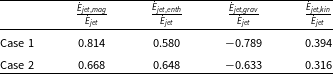

Figure 15. Time evolution of the ratio $\dot{E}_{jet,grav}\big / \dot{E}_{jet}$
of case 1 (
$\dot{E}_{jet,grav}\big / \dot{E}_{jet}$
of case 1 ( ${\unicode{x03D5}}_s= 0.002$
) and case 2 (
${\unicode{x03D5}}_s= 0.002$
) and case 2 ( ${\unicode{x03D5}}_s= 0.004$
).
${\unicode{x03D5}}_s= 0.004$
).

Figure 16. Temporal evolution of the ratio between the jet Poynting and kinetic flux $\dot{E}_{jet,mag}\big / \dot{E}_{jet,kin}$
of case 1 (
$\dot{E}_{jet,mag}\big / \dot{E}_{jet,kin}$
of case 1 ( ${\unicode{x03D5}}_s= 0.002$
) and case 2 (
${\unicode{x03D5}}_s= 0.002$
) and case 2 ( ${\unicode{x03D5}}_s= 0.004$
).
${\unicode{x03D5}}_s= 0.004$
).

Figure 17. Log-magnitude distribution of the energy power $ \dot E= \frac{1}{2} U^2 {\unicode{x03C1}} \boldsymbol{U} + \Phi_g {\unicode{x03C1}} \boldsymbol{U} + \boldsymbol{E} \times \boldsymbol{B} + \frac{{\unicode{x03B3}}}{{\unicode{x03B3}}-1} P \boldsymbol{U}$
in the disc–jet system of case 1 (
$ \dot E= \frac{1}{2} U^2 {\unicode{x03C1}} \boldsymbol{U} + \Phi_g {\unicode{x03C1}} \boldsymbol{U} + \boldsymbol{E} \times \boldsymbol{B} + \frac{{\unicode{x03B3}}}{{\unicode{x03B3}}-1} P \boldsymbol{U}$
in the disc–jet system of case 1 ( ${\unicode{x03D5}}_s= 0.002$
) for dynamical time steps (from top to bottom):
${\unicode{x03D5}}_s= 0.002$
) for dynamical time steps (from top to bottom): $t = 0$
,
$t = 0$
, $t = 50$
,
$t = 50$
, $t = 300$
and
$t = 300$
and $t = 700$
.
$t = 700$
.
In Fig. 18 of our study, we expand the scope of our visualisation to encompass the temporal evolution of log-magnitudes pertaining to the mechanical $ \dot{E}_{mec} = \frac{1}{2} U^2 {\unicode{x03C1}} \boldsymbol{U} + \Phi_g {\unicode{x03C1}} \boldsymbol{U}$
, magnetic
$ \dot{E}_{mec} = \frac{1}{2} U^2 {\unicode{x03C1}} \boldsymbol{U} + \Phi_g {\unicode{x03C1}} \boldsymbol{U}$
, magnetic $\dot{E}_{mag} = \boldsymbol{E} \times \boldsymbol{B} $
, and enthalpy
$\dot{E}_{mag} = \boldsymbol{E} \times \boldsymbol{B} $
, and enthalpy $\dot{E}_{enth} = \frac{{\unicode{x03B3}}}{{\unicode{x03B3}}-1} P \boldsymbol{U} $
components constituting the energy power
$\dot{E}_{enth} = \frac{{\unicode{x03B3}}}{{\unicode{x03B3}}-1} P \boldsymbol{U} $
components constituting the energy power $\dot E$
within the disc-jet system. Utilising distinct monochromatic colour gradients – green representing the mechanical component, blue depicting the magnetic component, and red signifying the enthalpy component – the first, second, and third rows of this representation respectively illustrate a comprehensive decomposition into these individual energy components. Examination of log-magnitude of each component underscores the importance of the enthalpy and mechanical elements throughout the entirety of the disc-jet system. Notably, the magnetic component exerts its significant influence primarily from the disc’s surface, where the jet begins to develop, to the end of our grid. This visualisation reaffirms our findings, emphasising the distinctive contributions made by each component to the overall energy
$\dot E$
within the disc-jet system. Utilising distinct monochromatic colour gradients – green representing the mechanical component, blue depicting the magnetic component, and red signifying the enthalpy component – the first, second, and third rows of this representation respectively illustrate a comprehensive decomposition into these individual energy components. Examination of log-magnitude of each component underscores the importance of the enthalpy and mechanical elements throughout the entirety of the disc-jet system. Notably, the magnetic component exerts its significant influence primarily from the disc’s surface, where the jet begins to develop, to the end of our grid. This visualisation reaffirms our findings, emphasising the distinctive contributions made by each component to the overall energy $\dot E$
. The composite in the fourth row distinctly reveals the simultaneous presence of all three components within the jet, illuminating their coexistence and interplay.
$\dot E$
. The composite in the fourth row distinctly reveals the simultaneous presence of all three components within the jet, illuminating their coexistence and interplay.
Upon scrutiny of Fig. 9, we unveiled a direct correlation between the temporal escalation in energy attributed to thermal conduction and the concurrent amplification in enthalpy energy. We noted that this observation emphasises that as local energy dissipation intensifies within the disc, the significance of enthalpy accretion flux grows at the expense of jet power. In order to elucidate this phenomenon further, we undertake a visualisation of the log-magnitude of $\dot E$
for both case 1 and case 2 at time steps
$\dot E$
for both case 1 and case 2 at time steps $t=300$
and
$t=300$
and $t=700$
(Fig. 19). Our examination reveals a discernible trend wherein the material power within the ejection zone of case 2 consistently registers lower values compared to those in case 1 over time. This evidence suggests that the augmentation of the saturation parameter
$t=700$
(Fig. 19). Our examination reveals a discernible trend wherein the material power within the ejection zone of case 2 consistently registers lower values compared to those in case 1 over time. This evidence suggests that the augmentation of the saturation parameter ${\unicode{x03D5}}_s$
leads to a gradual reduction in the jet’s power, elucidating an important correlation between this parameter and the jet power within the system.
${\unicode{x03D5}}_s$
leads to a gradual reduction in the jet’s power, elucidating an important correlation between this parameter and the jet power within the system.
4. Conclusions
This paper primarily focuses on examining the impact of saturated thermal conduction on angular momentum and energy transport in the disc-jet system. Utilising numerical simulations with the PLUTO code, we investigated the evolution of the disc-jet system and analysed the influence of various physical processes. By solving the time-dependent viscous resistive MHD equations, we incorporated a Shakura & Sunyaev (Reference Shakura and Sunyaev1973) alpha prescription and introduced a weak magnetic field threading the accretion disc. Our axisymmetric calculations allowed for long-term evolution, leading to the establishment of an accretion-ejection configuration. Through a consistent argumentation, we have demonstrated the importance of thermal conduction in the angular momentum and energy transport within the system.
Our initial focus was on examining the transport of angular momentum within the disc to gain insights into the magnetic and kinetic contributions to the total accretion angular momentum. Our investigation has revealed that the kinetic torque plays a significant role, making a major contribution to the total accretion angular momentum. On the other hand, the magnetic component, which acts to reduce the angular momentum, constitutes a relatively small contribution. These findings align with previous studies reported in the literature.
Moreover, our investigation revealed that thermal conduction plays a significant role at initial time steps by promoting accretion, leading to increased density in the inner region of the disc. This increased density indicates the availability of sufficient material for outward ejection. However, at advanced time steps of the simulations where the jet moves farther away from the disc, this effect is reversed. This behaviour can be attributed to the deceleration of the disc’s angular velocity caused by thermal conduction.
Our findings indicate that as the accretion-ejection structure becomes fully established, the significance of the viscous torque in angular momentum transport diminishes. Additionally, we observed that the impact of thermal conduction on the time evolution of the viscous torque is not substantial during the advanced stages of our calculations.
To evaluate the efficiency of the magnetocentrifugal mechanism, we investigated the ratio between the magnetic and kinetic torque. A higher ratio indicates a greater amount of specific angular momentum available at the disc’s surface, leading to an enhanced centrifugal acceleration and higher poloidal terminal speeds of the plasma. Our analysis unveiled that the increase of the saturation parameter strongly influences the magnitude of this ratio. Specifically, we found that at advanced times of the simulations, the magnetic contribution progressively surpasses the kinetic contribution, becoming increasingly dominant.
The temporal progression of the total accretion power showcases a well-stocked disc with an efficient inflow process. Our study demonstrated the substantial impact of thermal conduction within the system, as it amplifies the energy content within the control volume, resulting in an overall increase in energy output. We also focused on assessing the importance of energy derived from the enthalpy flux and mechanical power in relation to the overall accretion power. We discovered that the primary contribution originates from the mechanical flux, while the enthalpy energy contribution becomes increasingly significant over time. Furthermore, our findings revealed that the magnetic contribution is negligible. These results suggest a gradual shift in the relative importance of different energy sources involved in accretion as the system evolves, with thermal energy having a more prominent role.
We emphasised the crucial role of thermal conduction in promoting the pumping of material towards the vicinity of the central object while simultaneously reducing local energy dissipation. As a result, the presence of thermal conduction prevents the accumulation of enthalpy within the disc. To understand the total released energy within the disc, we examined the contribution of energy resulting from thermal conduction. Our analysis demonstrated the significant impact of thermal conduction on energy transport. Furthermore, we revealed that increasing the saturation parameter enhances this contribution.

Figure 18. Time evolution of log-magnitude of the mechanical component $\big \vert \dot{E}_{mec} = \frac{1}{2} U^2 {\unicode{x03C1}} \boldsymbol{U} + \Phi_g {\unicode{x03C1}} \boldsymbol{U} \big \vert $
(first row), log-magnitude of the magnetic component
$\big \vert \dot{E}_{mec} = \frac{1}{2} U^2 {\unicode{x03C1}} \boldsymbol{U} + \Phi_g {\unicode{x03C1}} \boldsymbol{U} \big \vert $
(first row), log-magnitude of the magnetic component $\big \vert \dot{E}_{mag} = \boldsymbol{E} \times \boldsymbol{B} \big \vert $
(second row), log-magnitude of the enthalpy component
$\big \vert \dot{E}_{mag} = \boldsymbol{E} \times \boldsymbol{B} \big \vert $
(second row), log-magnitude of the enthalpy component $\big \vert \dot{E}_{enth} = \frac{{\unicode{x03B3}}}{{\unicode{x03B3}}-1} P \boldsymbol{U} \big \vert $
(third row) and visual overlay of the sum of three components: log
$\big \vert \dot{E}_{enth} = \frac{{\unicode{x03B3}}}{{\unicode{x03B3}}-1} P \boldsymbol{U} \big \vert $
(third row) and visual overlay of the sum of three components: log $\big \vert \dot{E}_{mec} \big \vert$
+ log
$\big \vert \dot{E}_{mec} \big \vert$
+ log $\big \vert \dot{E}_{mag} \big \vert$
+ log
$\big \vert \dot{E}_{mag} \big \vert$
+ log $\big \vert \dot{E}_{enth} \big \vert$
(fourth row), in the disc–jet system of case 1 (
$\big \vert \dot{E}_{enth} \big \vert$
(fourth row), in the disc–jet system of case 1 ( ${\unicode{x03D5}}_s= 0.002$
).
${\unicode{x03D5}}_s= 0.002$
).

Figure 19. Log-magnitude distribution of the energy power $ \dot E= \frac{1}{2} U^2 {\unicode{x03C1}} \boldsymbol{U} + \Phi_g {\unicode{x03C1}} \boldsymbol{U} + \boldsymbol{E} \times \boldsymbol{B} + \frac{{\unicode{x03B3}}}{{\unicode{x03B3}}-1} P \boldsymbol{U}$
in the disc–jet system of case 1 (
$ \dot E= \frac{1}{2} U^2 {\unicode{x03C1}} \boldsymbol{U} + \Phi_g {\unicode{x03C1}} \boldsymbol{U} + \boldsymbol{E} \times \boldsymbol{B} + \frac{{\unicode{x03B3}}}{{\unicode{x03B3}}-1} P \boldsymbol{U}$
in the disc–jet system of case 1 ( ${\unicode{x03D5}}_s= 0.002$
) and case 2 (
${\unicode{x03D5}}_s= 0.002$
) and case 2 ( ${\unicode{x03D5}}_s= 0.004$
) for dynamical time steps
${\unicode{x03D5}}_s= 0.004$
) for dynamical time steps $t = 300$
(top panel) and
$t = 300$
(top panel) and $t = 700$
(bottom panel).
$t = 700$
(bottom panel).
We showed that the gradual increase in energy resulting from thermal conduction corresponds to a proportional rise in enthalpy energy over time. As the local energy dissipation within the disc intensifies, the significance of the enthalpy accretion flux increases at the expense of the jet power. This observation suggests a direct influence on the amount of energy extracted by the bipolar outflow from the disc.
The investigation into the temporal evolution of the ratio between the power of the jet and the power released in the disc reveals that the outflow is incapable of extracting the entire energy. This is different from cold jets, where the enthalpy flux is consistently insignificant and most of the power from accretion is released through the outflow pathway. We have highlighted two main factors that contribute to this behaviour. Firstly, the disc is traversed by a weak magnetic field that lacks the ability to extract a significant portion of the available power. Secondly, as the dissipation of turbulent energy intensifies within the disc, the enthalpy flux carried by accretion towards the central object becomes comparable to the jet power.
To unveil the intricate energy dynamics within the jet, it is of paramount importance to illuminate the myriad factors that contribute to the overall jet power. By doing so, we can delve into a more comprehensive analysis, drawing closer to identifying the major players in this enthralling phenomenon. Through our rigorous evaluation of individual components comprising the total jet power, we have unearthed compelling evidence that unequivocally establishes the Poynting flux as the primary contributor. Furthermore, we found that thermal conduction plays a negligible role in influencing the magnetic contribution to the total jet power.
We highlighted the importance of integrating jet enthalpy as another significant factor influencing the overall jet power. Specifically, we have established a strong connection between the rise in the saturation parameter and the amplification of the jet’s enthalpy contribution. This intriguing relationship unravels the intricate interplay between the saturation parameter, jet temperature, and the resulting enthalpy contribution.
In the context of examining how the ratio between the jet’s Poynting flux and kinetic flux evolves over time, we highlighted that a higher ratio indicates a larger amount of magnetic energy available per particle at the surface of the disc. This availability facilitates the acceleration of the outflow. We demonstrated that the Poynting flux, originating from the disc surface, effectively transforms into kinetic energy. Additionally, we indicated that the existence of thermal conduction promotes the prevalence of Poynting flux over kinetic flux during advanced time steps of our simulations.
This study provides comprehensive insights into the transport of angular momentum, energy dynamics, and the role of thermal conduction in accretion and jet formation. These findings deepen our understanding of these complex astrophysical processes and contribute to the growing knowledge of magnetohydrodynamic systems in the context of accreting objects.
The findings presented in this study pave the way for intriguing avenues of future research. The outcomes discussed herein offer a springboard for delving deeper into the intricate dynamics of the system under consideration. A forthcoming article will undertake a comprehensive examination of the interplay between saturated thermal conduction and its impact on the circulation of current within the disc-outflow system, thereby contributing significantly to the advancement of our comprehension regarding the accretion-ejection mechanism. Moreover, an in-depth analysis of the evolution of magnetic surfaces in both resistive and ideal zones, within the context of thermal conduction, emerges as a prominent avenue for exploration. This exploration promises to shed light on the nuanced behaviour of magnetic surfaces, elucidating their evolution under varied conditions and facilitating a deeper understanding of their role in the overall dynamics of the system. These future endeavours aim to unravel previously unexplored facets, providing valuable insights into the complex interplay of physical processes governing such systems.
Data availability statement
The data underlying this article were accessed from the Salomon supercomputer of IT4Inno–vations National Supercomputing Center, Czech Republic (https://www.it4i.cz/en/about/about-it4i). The derived data generated in this research will be shared on reasonable request to the corresponding author. PLUTO code is freely distributed under the GNU public licence, and it is available for download to the astrophysical community at the URL http://plutocode.to.astro.it.
Acknowledgement
We thank Andrea Mignone and the PLUTO team for the possibility to use their code. We express our sincere gratitude to the anonymous reviewer for devoting his time and expertise to thoroughly evaluate our article. His insightful and constructive comments contributed significantly to improving the clarity and presentation of our work. This work was supported by The Ministry of Education, Youth and Sports from the Large Infrastructures for Research, Experimental Development and Innovations project ‘IT4Innovations National Supercomputing Center – LM2015070’.
Funding statement
This research received no specific grant from any funding agency, commercial, or not-for-profit sectors.
Competing interests
None.
Appendix A. Units and Normalisation
Below, we state the corresponding units in a young stellar object (YSO). The main normalisation units are the Keplerian speed at the inner disc radius $r_{in}$
:
$r_{in}$
:
 \begin{equation} V_{k,in}=94 \Big(\frac{M}{M\odot} \Big)^\frac{1}{2} \Big(\frac{r_{in}}{0.1\, {\rm au}}\Big)^\frac{-1}{2} \quad {\rm km}\,{\rm s}^{-1} \end{equation}
The time unit is written as follows to correspond to the two aforementioned scales:
 \begin{equation} t_{in}=1.7 \Big(\frac{M}{M_\odot}\Big)^\frac{-1}{2} \Big(\frac{r_{in}}{0.1\,{\rm au}}\Big)^\frac{3}{2} \quad d \end{equation}
The accretion rate unit is based on the appropriate choice of the density normalisation ${\unicode{x03C1}}_{d,in}$
:
${\unicode{x03C1}}_{d,in}$
:
 \begin{equation} \dot{M}_{in} = r_{in}^2 {\unicode{x03C1}}_{d,in} V_{k,in} \quad {\rm M}_\odot \,{\rm yr}^{-1} \end{equation}
 \begin{equation} \dot{M}_{in} = 3\times 10^{-7} \Big(\frac{{\unicode{x03C1}}_{d,in}}{10^{-12}\,{\rm gcm}^{-3}}\Big) \Big(\frac{M}{M_\odot} \Big)^\frac{1}{2} \end{equation}
 \begin{equation*} \Big(\frac{r_{in}}{0.1\,{\rm au}}\Big)^\frac{3}{2} \quad {\rm M}_\odot\, {\rm yr}^{-1} \end{equation*}
After defining the initial thermal height scale with ${\unicode{x03B5}}$
parameter, the following quantity provides the normalisation value for temperature in the mid-plane:
${\unicode{x03B5}}$
parameter, the following quantity provides the normalisation value for temperature in the mid-plane:
 \begin{equation}T_{z=0} = {\unicode{x03B5}}^2 \frac{m_pGM}{kr} \quad K\end{equation}
 \begin{equation} T_{z=0} = 10^4 \Big(\frac{{\unicode{x03B5}}}{0.1}\Big)^2 \Big(\frac{M}{M_\odot}\Big) \Big(\frac{r_{in}}{0.1\,{\rm au}}\Big)^{-1} \quad K\end{equation}
The selection of the magnetisation parameter ( $B_{z=0} = \sqrt{8{\unicode{x03C0}} {\unicode{x03BC}} P}$
) controls the strength of the poloidal magnetic field at the equator:
$B_{z=0} = \sqrt{8{\unicode{x03C0}} {\unicode{x03BC}} P}$
) controls the strength of the poloidal magnetic field at the equator:
 \begin{equation} B_{z=0} = 2.6 \Big(\frac{{\unicode{x03BC}}}{{\unicode{x03BC}}_{d,in}}\Big)^\frac{1}{2}\Big(\frac{{\unicode{x03B5}}}{0.1}\Big) \Big(\frac{M}{M_\odot} \Big) ^\frac{1}{2} \Big(\frac{{\unicode{x03C1}}_{d,in}}{10^{-12}\,{\rm gcm}^{-3}}\Big) \end{equation}
 \begin{equation*} \Big (\frac{r_{in}}{0.1\,{\rm au}}\Big)^\frac{-5}{4} \quad G \end{equation*}
Torques are given in unit of $\dot{J}_{in}=r_{in}^3 {\unicode{x03C1}}_{d,in} V_{k,in}^2$
 \begin{equation} \dot{J}_{in} = 3\times 10^{38} \Big(\frac{{\unicode{x03C1}}_{d,in}}{10^{-12}\,{\rm gcm}^{-3}}\Big) \Big(\frac{M}{M_\odot} \Big) \Big(\frac{r_{in}}{0.1\,{\rm au}}\Big)^2 \quad dyne \, cm\end{equation}
Powers are given in unit of $\dot{E}_{in}=r_{in}^2 {\unicode{x03C1}}_{d,in} V_{k,in}^3$
 \begin{equation} \dot{E}_{in} = 1.9 \times 10^{33} \Big(\frac{{\unicode{x03C1}}_{d,in}}{10^{-12}\,{\rm gcm}^{-3}}\Big) \Big(\frac{M}{M_\odot} \Big)^\frac{3}{2} \Big(\frac{r_{in}}{0.1\,{\rm au}}\Big)^\frac{1}{2} \quad erg \,s^{-1}\end{equation}


