


1. Introduction
Particle electrification is ubiquitous in disperse two-phase flows, such as fluidized beds (Sippola et al. Reference Sippola, Kolehmainen, Ozel, Liu, Saarenrinne and Sundaresan2018) and pneumatic powder transports (Nifuku & Katoh Reference Nifuku and Katoh2003; Grosshans & Papalexandris Reference Grosshans and Papalexandris2016) in industrial processes, and sand saltation (Schmidt, Schmidt & Dent Reference Schmidt, Schmidt and Dent1998; Zheng, Huang & Zhou Reference Zheng, Huang and Zhou2003), dust storms (Yair et al. Reference Yair, Katz, Yaniv, Ziv and Price2016; Zhang & Zheng Reference Zhang and Zheng2018; Zhang & Zhou Reference Zhang and Zhou2020, Reference Zhang and Zhou2023) and volcanic eruptions (Mather & Harrison Reference Mather and Harrison2006; Méndez Harper & Dufek Reference Méndez Harper and Dufek2016) in atmospheric flows. Field and laboratory measurements regarding these phenomena have shown that the mean electric field produced by charged particles can reach strengths of several hundred kilovolts per metre, so that the inter-particle electrostatic force is comparable with the particle's gravitational force and thus affects the particle behaviour considerably (Renno & Kok Reference Renno and Kok2008). In particular, electrostatic force is found to facilitate the aerodynamic lifting of particles from the surface, by reducing the threshold friction velocity necessary to initiate particle lifting (e.g. Kok & Renno Reference Kok and Renno2006). Also, electrostatic force tends to enhance saltation mass flux when particles are negatively charged but inhibit the mass flux when particles are positively charged (Zheng et al. Reference Zheng, Huang and Zhou2003). Even though particle electrification has been observed and investigated for more than 100 years in natural conditions (e.g. Rudge Reference Rudge1913), it is not well understood because of the strong particle–turbulence and particle–electrostatics interphase couplings (e.g. Zheng Reference Zheng2013).
In wall-bounded turbulent flows laden with uncharged inertial particles, there is a tendency for particles to migrate towards the wall (i.e. the direction of negative gradient of turbulence intensity), resulting in a peak in mean particle concentration within the viscous layer, which is known as turbophoresis (Caporaloni et al. Reference Caporaloni, Tampieri, Trombetti and Vittori1975; Reeks Reference Reeks1983). This particle migration is thought to be most pronounced when the particle response time scale matches the characteristic time scale of the buffer layer (Soldati & Marchioli Reference Soldati and Marchioli2009; Sardina et al. Reference Sardina, Schlatter, Brandt, Picano and Casciola2012; Lee & Moser Reference Lee and Moser2015). Furthermore, it is well recognized that in low-Reynolds-number turbulent flows (typically with friction Reynolds number  $Re_\tau \sim O(10^2)$; see § 2.1 for the definition), inertial particles tend to aggregate preferentially into the regions of lower-than-mean streamwise velocity in the wall region, referred to as preferential concentration, which forms small-scale streak-like particle clustering and thus very non-uniform local particle concentration (e.g. Pedinotti, Mariotti & Banerjee Reference Pedinotti, Mariotti and Banerjee1992; Eaton & Fessler Reference Eaton and Fessler1994; Pan & Banerjee Reference Pan and Banerjee1996; Marchioli & Soldati Reference Marchioli and Soldati2002; Sardina et al. Reference Sardina, Schlatter, Brandt, Picano and Casciola2012). Such a small-scale streaky clustering is maximized when the particle response time scale is of the order of the Kolmogorov time scale (i.e. intermediate-inertia particles). For small- and large-inertia particles (i.e. particle response time scale much smaller or larger than the Kolmogorov time scale), they cannot form clustering, because the former particles follow the fluid faithfully, and the latter ones are almost independent of the flow. Note that in high-Reynolds-number turbulent flows (with $Re_\tau \gtrsim O(10^3)$), besides small-scale clustering for intermediate-inertia particles, large-scale clustering for the relatively large-inertia particles is present due to the presence of large-scale fluid motions (Oka & Goto Reference Oka and Goto2021; Jie et al. Reference Jie, Cui, Xu and Zhao2022; Motoori, Wong & Goto Reference Motoori, Wong and Goto2022). In fact, particle transfer in the wall region is dominated by the coherent sweep and ejection events, where the former carry particles towards the wall, while the latter bring particles away from the wall (Marchioli & Soldati Reference Marchioli and Soldati2002). Since only a fraction of particles that are entrained into the viscous sublayer by sweeps can be re-entrained towards the outer layer by ejections, the particle flux towards the wall is larger than the particle flux away from the wall, resulting in non-uniform distribution and near-wall accumulation of particles (Soldati & Marchioli Reference Soldati and Marchioli2009; Sardina et al. Reference Sardina, Schlatter, Brandt, Picano and Casciola2012; Costa, Brandt & Picano Reference Costa, Brandt and Picano2020; Brandt & Coletti Reference Brandt and Coletti2022).
It is expected that when particles are electrically charged, their behaviour could be altered considerably. Although particle electrification has been neglected for a long time in the study of particle-laden turbulent flows, it has continued to attract a lot of attention in the last two decades, due to recent advances in experimental facilities and direct numerical simulations (DNS). A large number of existing works focus on the influences of electrostatic forces on particle clustering in homogeneous isotropic turbulence (HIT). For monodisperse like-charged particles in HIT, Alipchenkov, Zaichik & Petrov (Reference Alipchenkov, Zaichik and Petrov2004) proposed a statistical model based on the kinetic equation of the relative velocity of particle pairs, and revealed that clustering is suppressed appreciably. This mitigation of preferential concentration is confirmed adequately by subsequent DNS and laboratory experiments (e.g. Lu et al. Reference Lu, Nordsiek, Saw and Shaw2010; Karnik & Shrimpton Reference Karnik and Shrimpton2012; Lu & Shaw Reference Lu and Shaw2015; Yao & Capecelatro Reference Yao and Capecelatro2018). More recently, a DNS study by Boutsikakis, Fede & Simonin (Reference Boutsikakis, Fede and Simonin2022) found that electrostatic forces could inhibit the dispersion of like-charged particles in HIT, by decreasing the correlation between particle velocity and fluid acceleration, and destroying the particle–fluid covariance. In addition to monodisperse particles, Di Renzo & Urzay (Reference Di Renzo and Urzay2018) have investigated bidisperse oppositely charged particles in HIT that are widely encountered but poorly understood in actual conditions. They showed that when electrostatic forces are mild, the small-inertia negatively charged particles are aggregated preferentially into low-vorticity high-strain fluid regions, while the large-inertia positively charged particles are distributed randomly, leading to charge separation according to particle inertia (e.g. Cimarelli et al. Reference Cimarelli, Alatorre-Ibargüengoitia, Kueppers, Scheu and Dingwell2014; Zhang & Zhou Reference Zhang and Zhou2020). By contrast, when electrostatic forces are severe, the small-inertia negatively charged particles become more uniformly distributed and indistinguishable from the large-inertia positively charged particles. It is worth noting that these DNS works have not incorporated particle–turbulence two-way coupling and inter-particle collisions, but the two effects are believed to be significant even at relatively low bulk particle volume fractions (e.g. Wang, Wexler & Zhou Reference Wang, Wexler and Zhou2000; Sardina et al. Reference Sardina, Schlatter, Brandt, Picano and Casciola2012; Costa et al. Reference Costa, Brandt and Picano2020; Johnson Reference Johnson2020), because turbophoresis and clustering cause locally very high concentration and mass loading. Until now, only Grosshans and co-workers have studied the role of electrostatic forces in wall turbulence by DNS (e.g. Grosshans et al. Reference Grosshans, Bissinger, Calero and Papalexandris2021). They simulated monodisperse charged particles in turbulent duct flows and demonstrated that electrostatic forces dramatically suppress both the vortical motion of particles and particle–fluid streamwise momentum transfer. However, when considering particle–turbulence and particle–electrostatics interphase couplings, as well as inter-particle collisions, the distribution, dynamics and clustering of particles in the wall region discussed above are still largely unclear, especially for bidisperse flows. Specifically, do the electrostatic forces play a role in the particle-laden turbulent channel flows? How do the electrostatic forces influence particle behaviour? What are the underlying physical mechanisms responsible for the electrostatic effects?
In this study, the main aims are twofold: (1) to quantify the role of electrostatic forces in the behaviour of the monodisperse and bidisperse particles embedded in low-Reynolds-number turbulent channel flows; and (2) to unveil the underlying physical mechanism responsible for the electrostatic effects. For these purposes, we perform a series of DNS of turbulent channel flows at  $Re_\tau =550$ laden with both monodisperse and bidisperse charged particles, in which the particle–turbulence and particle–electrostatics two-way couplings, as well as inter-particle collisions, are taken into account explicitly. The paper is organized as follows. First, the numerical model is described in §§ 2.1–2.3, and simulation set-up and verification are provided in detail in § 2.4 and Appendix A, respectively. Second, the roles of electrostatic forces in particles’ distribution, dynamics and clustering are discussed in §§ 3.1, 3.2 and 3.3, respectively. Finally, conclusions and an outlook on future work are given in § 4.
2. Numerical methodology
2.1. Turbulent channel flow
We simulate the aforementioned particle-laden turbulent channel flows using a coupled Eulerian–Lagrangian point-particle approach supplemented with electrostatic equations, since the particles considered herein are dilute suspension and small compared to the Kolmogorov scale (e.g. Maxey & Riley Reference Maxey and Riley1983; Maxey Reference Maxey1987; Balachandar Reference Balachandar2009). In such a case, the incompressible Newtonian carrier fluid is governed by the mass and momentum balance equations as
 $$\begin{gather} \boldsymbol{\nabla}\boldsymbol{\cdot} \boldsymbol{u} = 0, \end{gather}$$
 $$\begin{gather}\frac{\partial \boldsymbol{u}}{\partial t}+(\boldsymbol{u}\boldsymbol{\cdot}\boldsymbol{\nabla})\boldsymbol{u} ={-}\frac{1}{\rho_f}\,\boldsymbol{\nabla} p+\nu\,\nabla^2 \boldsymbol{u}+\boldsymbol{f}, \end{gather}$$
where  $\boldsymbol {u}=(u,v,w)$ and $\boldsymbol {x}=(x,y,z)$ represent the fluid velocity and spatial coordinate, respectively, with $u$,
$u$,  $v$ and $w$ (
$w$ ( $x$,
$x$,  $y$ and $z$) being the streamwise, wall-normal and spanwise velocities (coordinates). In addition, $t$ stands for the physical time, and $\rho _f$, $p$ and $\nu$ denote the fluid density, pressure and kinematic viscosity, respectively. The source term $\boldsymbol {f}$ is added to account for the feedback force exerted by the particles on the fluid, which is calculated as (Marshall Reference Marshall2009; Zhao, Andersson & Gillissen Reference Zhao, Andersson and Gillissen2013; Zheng, Feng & Wang Reference Zheng, Feng and Wang2021)
 \begin{equation} \boldsymbol{f} ={-}\frac{1}{\rho_f\,V_{cell}}\sum_{k=1}^{n_p}\boldsymbol{f}_{D}^k. \end{equation}
Here,  $\boldsymbol {f}_{D}^k$ is the hydrodynamic drag force acting on the $k$th particle within a computational cell of volume $V_{cell}$ containing $n_p$ particles.
We consider turbulent channel flow that is driven by a uniform pressure gradient, such that a constant bulk velocity is maintained. The dimensionless control parameter, i.e. the friction Reynolds number, is defined as  $Re_\tau =u_\tau \delta /\nu$, where $u_\tau$ is the friction velocity, and $\delta$ is the channel half-width. Throughout this paper, the superscript $+$ denotes quantities that are normalized based on $u_\tau$ and $\nu$ (i.e. in viscous or wall units, such as time $\tau _\nu =\nu /u_\tau ^2$ and length $\delta _\nu =\nu /u_\tau$ scales). Periodic boundary conditions in the horizontal (i.e. streamwise and spanwise) directions and no-slip boundary conditions at the wall are employed. Equations (2.1) and (2.2) are solved based on the canonical Navier–Stokes solver (CaNS) developed by Costa (Reference Costa2018), using a fast Fourier transform (FFT) based pressure correction method (Kim & Moin Reference Kim and Moin1985). A standard second-order central finite-difference scheme is used for the space discretization on a staggered Cartesian mesh. Time is advanced with a third-order Runge–Kutta scheme. The solution of the Poisson equation for the pressure correction is based on the eigenfunction expansion method (Schumann & Sweet Reference Schumann and Sweet1988). The FFT-based expansions are employed in the horizontal, uniformly discretized directions, then Gaussian elimination is used to solve the resulting tridiagonal system along the wall-normal direction.
2.2. Lagrangian particle tracking
For the particulate phase, we consider small, rigid, charged or uncharged, and spherical particles that are suspended in the turbulent channel flow. The particle density  $\rho _p$ (particle diameter $d_p$) is taken to be much larger than $\rho _f$ (smaller than the Kolmogorov scale), so that the point-particle approximation is quite reasonable and the Stokes drag force is the dominant hydrodynamic force on the particle (Maxey & Riley Reference Maxey and Riley1983; Armenio & Fiorotto Reference Armenio and Fiorotto2001; Balachandar & Eaton Reference Balachandar and Eaton2010). To emphasize the effects of particle inertia and electrostatic forces, gravitational settling is not taken into account (e.g. Wang & Richter Reference Wang and Richter2019; Jie et al. Reference Jie, Cui, Xu and Zhao2022; Motoori et al. Reference Motoori, Wong and Goto2022). Consequently, in the Lagrangian description, each particle is tracked individually using the governing equations as
 $$\begin{gather} \frac{\mathrm{d}\boldsymbol{x}_{p}}{\mathrm{d} t} = \boldsymbol{u}_{p}, \end{gather}$$
 $$\begin{gather}\frac{\mathrm{d} \boldsymbol{u}_{p}}{\mathrm{d} t} = \frac{\zeta}{\tau_p}\,(\boldsymbol{u}_{f@p}-\boldsymbol{u}_{p})+\frac{q\boldsymbol{E}_{@p}}{m_p}, \end{gather}$$
where  $\boldsymbol {x}_{p}$ is the particle position, $\boldsymbol {u}_{p}$ is the particle velocity, $\zeta =1+0.15\,Re_p^{0.687}$ with $Re_p=d_p\,| \boldsymbol {u}_{f@p} - \boldsymbol {u}_{p} |/\nu$ being the particle Reynolds number (Schiller & Naumann Reference Schiller and Naumann1935; Lavrinenko, Fabregat & Pallares Reference Lavrinenko, Fabregat and Pallares2022), $\tau _p=d_p^2\rho _p/(18\nu \rho _f)$ is the particle inertial response time (e.g. Maxey Reference Maxey1987; Eaton & Fessler Reference Eaton and Fessler1994), $\boldsymbol {u}_{f@p}$ is the fluid velocity at the particle position, $q$ is the electric charge of the particle, $\boldsymbol {E}_{@p}$ is the electric field at the particle position, and $m_p={\rm \pi} \rho _p d_p^3/6$ is the particle mass.
From (2.5), there are two dimensionless parameters controlling the particle dynamics. One is the viscous (or Kolmogorov) aerodynamic Stokes number  $St^+=\tau _p/\tau _\nu$ ( $St_k=\tau _p/\tau _\eta$), which is defined as the ratio of the particle inertial response time $\tau _p$ to the viscous time scale $\tau _\nu$ (Kolmogorov time scale $\tau _\eta$). The other parameter, termed the electrostatic Stokes number, is defined as $St_{el}=\tau _p/\tau _{el}$, where $\tau _{el}=(6{\rm \pi} \varepsilon _0m_p/(nq^2))^{1/2}$ stands for the characteristic time scale of the inter-particle electrostatic interactions (Boutsikakis et al. Reference Boutsikakis, Fede and Simonin2022), with $n$ and $\varepsilon _{0}$ being the particle number density and the permittivity of the vacuum, respectively. The two parameters weigh the importance of particle inertia and electrostatic forces. In particular, particles will attain a ballistic motion when the aerodynamic Stokes number is much larger than unity, but become tracers when the aerodynamic Stokes number is much smaller than unity. Also, the inter-particle electrostatic forces are dominating (negligible) if the electrostatic Stokes number is much larger (smaller) than unity.
Similarly, we impose periodic boundary conditions for particles in the horizontal directions, and reflective boundary conditions for particles on the top and bottom walls. A particle–wall collision occurs when the distance between the particle centre and the wall is less than the particle radius. Inter-particle collisions are also taken into account since preferential concentration and turbophoresis lead to a locally very high particle concentration (e.g. Wang et al. Reference Wang, Wexler and Zhou2000; Yamamoto et al. Reference Yamamoto, Potthoff, Tanaka, Kajishima and Tsuji2001). Unless stated otherwise, both particle–wall and inter-particle collisions are assumed to be fully elastic (thus conserving kinetic energy) and are described using the ‘hard-sphere’ approach, as in many previous studies (e.g. Marchioli & Soldati Reference Marchioli and Soldati2002; Sardina et al. Reference Sardina, Schlatter, Brandt, Picano and Casciola2012; Johnson, Bassenne & Moin Reference Johnson, Bassenne and Moin2020; Motoori et al. Reference Motoori, Wong and Goto2022). Therefore, when colliding with the wall, the tangential velocity of the particle remains unchanged and the wall-normal component is of the same magnitude but opposite direction (i.e. reflective). Notably, particle collisions in a viscous fluid are actually inelastic, with restitution coefficient smaller than unity (e.g. Rice, Willetts & McEwan Reference Rice, Willetts and McEwan1995; Joseph et al. Reference Joseph, Zenit, Hunt and Rosenwinkel2001; Gondret, Lance & Petit Reference Gondret, Lance and Petit2002; Yang & Hunt Reference Yang and Hunt2006). However, the differences in the results between inelastic and elastic collisions considered herein are found to be negligible (e.g. Sardina et al. Reference Sardina, Schlatter, Brandt, Picano and Casciola2012; Johnson et al. Reference Johnson, Bassenne and Moin2020).
Only binary inter-particle collisions are considered due to dilute particle loading. Thus, considering that two particles labelled as 1 and 2 with velocities  $\boldsymbol {u}_{p,1}$ and $\boldsymbol {u}_{p,2}$ collide with each other, the post-collision velocity of particle 1 is given by (Grosshans & Papalexandris Reference Grosshans and Papalexandris2017a)
 \begin{equation} \boldsymbol{u}_{p,1}^{post}=\frac{\boldsymbol{u}_{p,1}(m_{p,1}-m_{p,2})+2m_{p,2}\boldsymbol{u}_{p,2}}{m_{p,1}+m_{p,2}}, \end{equation}
where  $m_{p,1}$ and $m_{p,2}$ are the masses of particles 1 and 2, respectively. For particle 2, post-collision velocity is obtained by permutation of the indices 1 and 2.
Time integration of (2.4) and (2.5) is performed using a fourth-order Runge–Kutta scheme. Inter-particle collisions are detected by the Eulerian-mesh-based method, in which the potential colliding particle pairs are found in the target and its neighbouring cells (for the details, see Capecelatro & Desjardins Reference Capecelatro and Desjardins2013).
2.3. Electric fields
The electric field at each particle position is calculated by the particle-particle-particle-mesh ( ${\rm P}^3{\rm M}$) method, encompassing long-range component accounting for far-field effects, short-range component accounting for neighbouring particles, and a correction term to exclude double counting of the former two (Kolehmainen et al. Reference Kolehmainen, Ozel, Boyce and Sundaresan2016; Grosshans & Papalexandris Reference Grosshans and Papalexandris2017b; Sippola et al. Reference Sippola, Kolehmainen, Ozel, Liu, Saarenrinne and Sundaresan2018). Considering particle $i$ located at $\boldsymbol {x}_i$, the long-range component $\boldsymbol {E}_{\nabla ^2}$ can be determined by projecting particles to the computational mesh and solving the Poisson equation for the electrical potential:
 $$\begin{gather} \nabla^2 \varphi ={-}\frac{\rho_{e}}{\varepsilon_0}, \end{gather}$$
 $$\begin{gather}\boldsymbol{E}_{\nabla^2} ={-}\boldsymbol{\nabla}\varphi, \end{gather}$$
where  $\varphi$ is the electric potential, and $\rho _e=\sum _{k=1}^{n_p}q_k/V_{cell}$ is the space-charge density. Note that this Eulerian formulation has been used solely for quantifying the electrostatic forces acting on particles through interpolation, as in Karnik & Shrimpton (Reference Karnik and Shrimpton2012), Kolehmainen, Ozel & Sundaresan (Reference Kolehmainen, Ozel and Sundaresan2018) and Grosshans et al. (Reference Grosshans, Bissinger, Calero and Papalexandris2021). Again, the periodic boundary conditions are applied to electrical potential in the horizontal directions, but zero-Dirichlet conditions ( $\varphi =0$) are set at the wall. Equation (2.7) is resolved by the same algorithm as used for the Poisson equation of pressure correction.
As done in Sippola et al. (Reference Sippola, Kolehmainen, Ozel, Liu, Saarenrinne and Sundaresan2018), the short-range component  $\boldsymbol {E}_{s,i}$ for particle $i$ within computational cell $A$ is determined directly by Coulomb's law
 \begin{equation} \boldsymbol{E}_{s, i}=\frac{1}{4 {\rm \pi}\varepsilon_0} \sum_{j\neq i} q_j\, \frac{\boldsymbol{x}_i-\boldsymbol{x}_j}{|\boldsymbol{x}_i-\boldsymbol{x}_j|^3}, \end{equation}
where the sum is taken over all neighbouring particles  $j$ carrying charge $q_j$ located in cell $A$ and its adjacent cells.
To avoid double counting of the overlap of long- and short-range components, a correction term is introduced as
 \begin{equation} \boldsymbol{E}_{c, A}={-}\frac{1}{4 {\rm \pi}\varepsilon_0} \sum_{B\neq A} Q_B\, \frac{\boldsymbol{x}_A-\boldsymbol{x}_B}{|\boldsymbol{x}_A-\boldsymbol{x}_B|^3}, \end{equation}
where the sum is performed over all adjacent cells  $B$ of cell $A$,
$A$,  $Q_B$ is the total charge enclosed within cell $B$, and $\boldsymbol {x}_A$ and $\boldsymbol {x}_B$ are the coordinates of the centre of the cell.
2.4. Simulation set-up
The simulations to be discussed in the present study are performed at  $Re_\tau =550$. The computational domain is set as $2{\rm \pi} \delta \times 2\delta \times {\rm \pi}\delta$, which is large enough to capture accurately particle behaviours even at $Re_\tau$ from 1000 to 5186 (Jie et al. Reference Jie, Cui, Xu and Zhao2022; Motoori et al. Reference Motoori, Wong and Goto2022; Gao, Samtaney & Richter Reference Gao, Samtaney and Richter2023). Detailed information on the selection of such a computational domain can be found in Gao et al. (Reference Gao, Samtaney and Richter2023). A total of $384\times 384\times 256$ grid points are used to discretize the computational domain. The grid spacing is uniform in the horizontal directions, with $\Delta x_g^+\approx 9.00$ and $\Delta z_g^+\approx 6.75$. However, a stretched grid is used to refine the grid close to the wall, thus $\Delta y_g^+$ varies approximately from 0.43 to 4.75. The grid parameters are summarized in table 1.
Table 1. Grid parameters for the DNS. Here,  $L_x$, $L_y$ and $L_z$ are the streamwise, wall-normal and spanwise computational domain sizes, respectively, $\delta =0.2$ m is the channel half-width, $N_x$, $N_y$ and $N_z$ are the numbers of grid points, and $\Delta x_g^+$, $\Delta y_g^+$ and $\Delta z_g^+$ are the grid spacings normalized by the viscous length scale $\nu /u_\tau$.
To uncover the effects of electrostatic forces on particle behaviour, we consider both monodisperse and bidisperse particles embedded in the turbulent channel flows with five different electrostatic Stokes numbers, as shown in table 2. For the monodisperse cases, the aerodynamic number is specified as  $St^+=20$, at which the near-wall particle streaks are very prominent. In each case, a total number of $N=2\times 10^6$ particles carry an identical electrical charge $q$ ranging from 0 to $-0.01$ pC, corresponding to the bulk mean electrostatic Stokes number in the range $\overline{St_{el}} \in [0, 0.59\times 10^{-2}]$. By contrast, two classes of particles are examined in the bidisperse cases, where the lighter particles, $St^+=20$, are negatively charged, while the heavier ones, $St^+=400$, are positively charged with equal magnitude (from 0 to 0.1 pC). As a result, the bulk mean electrostatic Stokes number $\overline{St_{el}}$ varies from 0 to $4.14\times 10^{-2}$ (0 to $1.85\times 10^{-1}$) for the lighter (heavier) particles. These $\overline{St_{el}}$ values are of the same order as those used in Di Renzo et al. (Reference Di Renzo, Johnson, Bassenne, Villafañe and Urzay2019) and Grosshans et al. (Reference Grosshans, Bissinger, Calero and Papalexandris2021), but one order of magnitude smaller than those used in Boutsikakis et al. (Reference Boutsikakis, Fede and Simonin2022). The given maximum electrical charge (i.e. 0.1 pC) is approximately a quarter of the saturation charge on the particles $q_s=0.44$ pC ( $q_s={\rm \pi} d_p^2E_{sat}\varepsilon _0$), which is limited by the dielectric breakdown of the carrier fluid with breakdown field strength $E_{sat}=3\times 10^3\ {\rm kV}\ {\rm m}^{-1}$ (e.g. Hamamoto, Nakajima & Sato Reference Hamamoto, Nakajima and Sato1992). Note that charge exchanges during inter-particle and particle–wall collisions are not taken into account, as done by Di Renzo & Urzay (Reference Di Renzo and Urzay2018), Grosshans et al. (Reference Grosshans, Bissinger, Calero and Papalexandris2021) and Boutsikakis et al. (Reference Boutsikakis, Fede and Simonin2022). This is because there is no consensus on how the electrical charge is distributed among particles, which is very sensitive to the selection of charge exchange model (Lacks & Sankaran Reference Lacks and Sankaran2011). The bidisperse particles are equally repartitioned among the two classes (i.e. $1\times 10^6$ particles for each class), keeping the system electrically neutral (Di Renzo & Urzay Reference Di Renzo and Urzay2018). The particle diameters considered in both monodisperse and bidisperse cases are fixed at $d_p^+=0.2$ (i.e. $d_p=72.7\ \mathrm {\mu }{\rm m}$), which is smaller than the Kolmogorov length scales of the simulated flows and the minimum grid spacing $\Delta y_{min}^+\approx 0.43$, so the point-particle approach is applicable (Horwitz & Mani Reference Horwitz and Mani2016). Accordingly, the particle-to-fluid density ratio is $\rho _p/\rho _f=9\times 10^3$ for the lighter particles, and $\rho _p/\rho _f=1.8\times 10^5$ for the heavier particles. It is noteworthy that even though such large particle-to-fluid density ratios are rarely encountered in natural phenomena, the particles with the same controlling parameters ( $St^+$ and $St_{el}$) at common density ratios are expected to experience identical dynamics.
Table 2. Main parameters for the particles. Here,  $\overline{\phi_m}$, $\overline{\phi_v}$ and $\overline{St_{el}}$ represent the bulk mean particle mass loading ratio, particle volume fraction and electrostatic Stokes number, respectively. The particle Stokes numbers $St^+$ and $St_k$ are calculated based on the viscous and Kolmogorov time scales, respectively, where the subscript max (min) refers to the maximum (minimum) $St_k$ at the wall (channel centreline).

Each simulation is started from a fully developed turbulent flow at dimensionless time  $t^+=0$ ( $t^+=t/t_\nu$) and is terminated at $t^+\approx 29\,250$. Such a considerable long-time simulation is necessary to ensure that a statistically steady state for the particulate phase is attained, which is evidenced by the evolution of the Shannon entropy of particle distribution (see Appendix B for the details). The particles are released randomly in the entire computational domain at $t^+=0$. The initial velocity of each particle is set to be the fluid velocity at the particle position. The boundary conditions used in the present study are detailed in §§ 2.1–2.3 and illustrated by figure 1. For all statistics, the ensemble averaging, denoted by $\langle \cdot \rangle$, is performed over the horizontal directions and time hereafter. Here, 10 equally spaced snapshots in the time interval $t^+\in [27\,300,29\,250]$ are used for time averaging. The validation of our numerical simulation is presented in Appendix A.

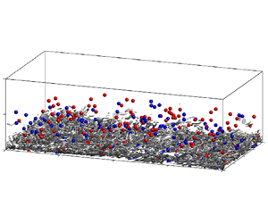
Figure 1. Sketch of the geometry and boundary conditions of the simulations. The periodic boundary conditions in the  $x$- and $z$-directions are applied to the carrier fluid, particulate phase and electrical potential. The no-slip, reflective and conducting boundaries at the top and bottom walls are applied to the carrier fluid, particulate phase and electrical potential, respectively. The isosurfaces of the $Q$-criterion are shown at $Q=150$ and are coloured by the streamwise velocity for the bidisperse case ${\rm BD}^\pm 0.006$ at $t^+\approx 29\,250$. For clarity, only isosurfaces in the lower half of the channel are shown. Particles with wall distance $y<0.2$ m are depicted in blue (red) for lighter (heavier) particles, where only every three thousand particles are shown.
3. Results and discussion
3.1. Role of electrostatic forces in particle distribution
To evaluate whether the electrostatic forces alter the particle distribution dramatically, we begin by comparing the instantaneous particle distributions of the uncharged and charged cases in various distinct wall-parallel planes, as displayed in figure 2. As reported previously, for the uncharged monodisperse case, the longitudinal particle streaks of length exceeding  $10^3\delta _\nu$ exist in the viscous layer (figure 2a, left) (e.g. Ninto & Garcia Reference Ninto and Garcia1996). Such streaks for the preferential concentration of particles become weaker in the buffer layer (figure 2b, left) and transition to cloud patterns in the outer layer (figure 2c, left). The formations of these clustering patterns are responsible for the fact that particles tend to aggregate into the low-speed velocity streaks in the near-wall region, but tend to collect in the high-speed regions in the outer layer (Marchioli & Soldati Reference Marchioli and Soldati2002; Sardina et al. Reference Sardina, Schlatter, Brandt, Picano and Casciola2012; Wang & Richter Reference Wang and Richter2019). When particles are highly charged (i.e. $q=-0.01$ pC and $\overline{St_{el}}=0.59\times 10^{-2}$), the clustering patterns in different wall-parallel planes seem to be obscured to the bare eye, due to the considerable reductions in the particle concentrations (figures 2a–c, right). The quantitative measures are given further in § 3.3.

Figure 2. Instantaneous snapshots of the particle distribution in the wall-parallel ( $x$–
$x$– $z$) plane at $t^+\approx 29\,250$ (not to scale). (a–c) Snapshots of the particle distributions in three layers $y^+ \in [2.1, 5.6]$, $[15.2,25.0]$ and $[530.5, 548.5]$, respectively, and streamwise velocity fluctuations ${u'}^+$ at $y^+=3.8$, 20.5 and 539.5, for the monodisperse cases MD0 and MD0.01 ( $St^+=20$). Here, the black dots depict the particles, and contours represent the fluctuating streamwise velocity. (d–f) Same as (a–c) but for bidisperse cases BD0 and BD $^\pm$0.1, where particles outside (inside) the white rectangles represent the lighter particles $St^+=20$ (heavier particles $St^+=400$). In each panel, the left-hand (right-hand) side represents the flow laden with uncharged (charged) particles.
By contrast, the electrostatic effects in the bidisperse cases are somewhat different. For the uncharged lighter particles with  $St^+=20$ (figures 2d–f, left), the same clustering patterns as in the uncharged monodisperse cases are observed as expected. However, the heavier particles with $St^+=400$ remain uniformly distributed (insets in figures 2d–f, left), owing to their very large inertia (i.e. see table 2, $St_{k,min}=10.1$, which is much larger than unity). In contrast to the monodisperse cases, the number densities of the lighter and heavier particles are slightly changed by electrostatic forces, even in the presence of a large amount of electrical charge on particles (i.e. $q=\pm 0.1$ pC; figures 2d–f, right). Importantly, the lighter particles become much more uniformly distributed in the viscous layer when particles are highly charged, demonstrating that electrostatic forces indeed affect the distribution of the small-inertia particles.
To further assess the effects of electrostatic forces quantitatively, the wall-normal profiles of the mean particle number density are plotted in figure 3. All particle number densities are normalized by the bulk mean number density  $n_0=N/(L_xL_yL_z)$. In the case of flow laden with monodisperse uncharged particles, the mean particle number density decreases with increasing wall-normal location $y^+$ (figure 3a). This tendency of particle migration to the wall is caused by turbophoresis, as demonstrated in previous studies (Caporaloni et al. Reference Caporaloni, Tampieri, Trombetti and Vittori1975; Reeks Reference Reeks1983; Marchioli et al. Reference Marchioli, Soldati, Kuerten, Arcen, Taniere, Goldensoph, Squires, Cargnelutti and Portela2008). When the electrical charge on particles increases from 0 to $-0.01$ pC, the particle number density in the bulk of the channel is reduced considerably, especially at $y^+\approx 1$, where it is decreased over two orders of magnitude. Meanwhile, the particle number density is increased substantially in a thin layer adjacent to the wall (i.e. $y^+\sim 0.2\unicode{x2013}0.3$), suggesting that electrostatic forces enhance the particle wall accumulation in the monodisperse cases.

Figure 3. Wall-normal profiles of the mean particle number density for the (a) monodisperse ( $St^+=20$) and (b) bidisperse ( $St^+=20$ and $St^+=400$) cases. The mean particle number density $\langle n \rangle$ is normalized by the bulk mean number density $n_0$. The solid and dashed lines in (b) denote the lighter ( $St^+=20$) and heavier ( $St^+=400$) particles, respectively. The open and filled symbols denote the particle concentrations predicted by (3.1) for the lighter and heavier particles, respectively.
In the bidisperse cases, wall-normal distributions of the lighter and heavier particles exhibit quite different behaviours. When particles are not electrically charged (i.e.  $q=0$), the wall accumulation of the lighter particles is remarkable, while the heavier ones are rather uniformly distributed along the wall-normal direction (figure 3b). As electrical charge increases, the particle number density profile becomes flatter (steeper) for the lighter (heavier) particles. More specifically, the number density of the lighter particles is decreased in the wall layer but increased in the bulk of the channel (i.e. counter-clockwise pivoting effect). In contrast, there is an opposite effect for the heavier particles (i.e. clockwise pivoting effect). Consequently, the combined effect of the electrostatic forces tends to mitigate the concentration difference between the lighter and heavier particles.
The physical mechanisms for determining particle transport in the wall-normal direction can be deduced from the theoretical formulation of particle concentration:
 \begin{align} n(y;t) & = C \exp \left( \underbrace{\frac{1}{\tau_p} \int_0^y \frac{\left\langle \zeta v_{f@p} | \xi \right\rangle}{\left\langle v_p^2 | \xi\right\rangle}\,\mathrm{d} \xi}_{\textit{biased\ sampling}} \right.\nonumber\\ &\quad + \left. \underbrace{\frac{q}{m_p} \int_0^y \frac{\left\langle E_{y@p} | \xi\right\rangle}{\left\langle v_p^2 | \xi\right\rangle}\,\mathrm{d} \xi}_{\textit{electrostatic forces}}-\underbrace{\int_0^y \frac{\mathrm{d} \ln \left\langle v_p^2 | \xi\right\rangle}{\mathrm{d} \xi}\,\mathrm{d} \xi}_{\textit{turbophoresis}} \right), \end{align}
which is derived from the kinetic equation for the single-point particle distribution function (Williams Reference Williams1958; Sikovsky Reference Sikovsky2014; Johnson et al. Reference Johnson, Bassenne and Moin2020). Detailed information is offered in Appendix C. In (3.1), three phoresis integrals can be defined. The first term on the right-hand side accounts for the biased sampling of fluid velocity by particles, the second term represents the electrostatic drift, and the third term accounts for the turbophoresis. Therefore, the particle concentration profile is determined by the competition of turbophoresis, biased sampling and electrostatic drift, which is evidenced in figure 3 (symbols). Notably, (3.1) is obtained by neglecting the momentum exchanges between the lighter and heavier particles for the bidisperse cases. Qualitative agreement of the theoretical predictions with simulation (figure 3b) indicates that these momentum exchanges are indeed negligible.
To explain why the wall-normal number density profiles of the monodisperse and bidisperse cases behave differently under the actions of electrostatic forces, the resulting three phoresis integrals are presented in figure 4. These integrals are computed numerically using a trapezoidal rule on a uniform grid with spacing  $0.42\delta _\nu$. It is shown that for the monodisperse and bidisperse cases, the biased sampling and turbophoresis integrals are both positive and increase with increasing wall-normal location. This occurs because particles tend to accumulate in low-speed streaks of fluid flow (i.e. $\langle \zeta v_{f@p} | y\rangle >0$) and there is a positive gradient of particle wall-normal velocity fluctuations (i.e. $\mathrm {d}\langle v_p^2 | y\rangle /\mathrm {d} y>0$). According to (3.1), it is recognized that biased sampling leads to particles moving away from the wall, while turbophoresis results in a migration of particles towards the wall.

Figure 4. (a–c) Comparisons between turbophoresis integrals ( $I_{turb}$, dashed lines) and electrostatic integrals ( $I_{elec}$, solid lines). (d–f) Comparisons between biased sampling integrals ( $I_{bias}$, dashed lines) and electrostatic integrals ( $I_{elec}$, solid lines). Here, (a,d) correspond to the monodisperse cases, and (b,e) and (c, f) correspond to the lighter and heavier particles in the bidisperse cases, respectively. Note that the electrostatic integrals are shown by their absolute values for clarity, where the solid (dotted) lines representing their actual values are negative (positive).
In monodisperse cases, electrostatic integrals are negative and nearly constant with the wall-normal location (figures 4a,d) because the mean wall-normal electric fields are directed towards the channel centreline and decrease sharply with increasing wall-normal location (not shown for brevity). Also, from (3.1), it is known that the wall-normal component of the electrostatic forces produces a drift of the particles to the wall and thus a considerable reduction of particle number density in the outer layer. This electrostatic drift is self-regulating, in which the particle number density in the outer layer declines until the wall-normal electric field is decreased to the point that an equilibrium transport is achieved. For the bidisperse cases, however, the electrostatic integrals of the lighter particles are negative in a thin layer close to the wall, but positive above this layer (figures 4b,e), even though those of heavier particles are negative (figures 4c, f). As a result, electrostatic forces produce a wall-pointing drift very close to the wall but a channel-centreline-pointing drift in the bulk of the channel for the lighter particles. This bulk channel-centreline-pointing drift prevents particles moving towards the wall, leading to a reduction in the number density of lighter particles close to the wall, although the lighter particles tend to be held by electrostatic forces in a thin layer close to the wall. By contrast, heavier particles experience a wall-pointing electrostatic drift in the whole channel. Such different electrostatic effects for lighter and heavier particles very close to the wall are caused by their significant concentration differences in this layer. Overall, the wall-normal component of the electrostatic forces causes a particle to drift away from (towards) the wall for the lighter (heavier) particles. Doubtless, such a bidirectional electrostatic drift is responsible for the variations of particle number density profile in the wall-normal direction; the details will be discussed in § 3.2.
We end this subsection by clarifying how the positions of the particles correlate with the fluid velocity fields at various values of particle charge. First, we examine the probability density functions (p.d.f.s) of the fluctuating streamwise fluid velocity at particle positions (i.e. conditioned velocity  ${u'}^+_{f@p}$) in the wall region, as shown in figure 5. It is clear that for the lighter particles in the uncharged monodisperse and bidisperse cases, the p.d.f.s of the conditioned velocity ${u'}^+_{f@p}$ deviate significantly from those of unconditioned fluctuating velocity ${u'}^+$. The p.d.f. peaks correspond to negative values of fluctuating streamwise fluid velocity, which verify quantitatively that lighter particles are trapped in the low-speed streaks of the fluid flow (Pedinotti et al. Reference Pedinotti, Mariotti and Banerjee1992; Marchioli & Soldati Reference Marchioli and Soldati2002). With increasing electrical charge, these p.d.f. peaks are slightly shifted towards zero and so suppress particle aggregation in the low-speed fluid streaks. The shifts in the buffer layer for the bidisperse cases are slightly larger compared to the monodisperse cases (e.g. figures 5c, f). The reason is that in the buffer layer, the local electrostatic Stokes numbers in the bidisperse cases are much larger than those in the monodisperse cases, as shown in figure 6. For the heavier particles in the bidisperse cases, the p.d.f.s of the conditioned and unconditioned velocities ${u'}^+_{f@p}$ and ${u'}^+$ are very similar, because the heavier particles are randomly distributed, and thus sample the fluid velocity fields uniformly. Also, the p.d.f. peaks are very close to zero and are unaffected by the electrostatic forces (insets in figures 5d–f). This is because electrostatic forces tend to homogenize the particle distribution in both monodisperse and bidisperse cases (as will be shown in § 3.3), so that does not alter the randomly distributed heavier particles. This result is in accordance with figures 2(d)–2( f).

Figure 5. (a–c) In turn, the probability density functions (p.d.f.s) of the fluctuating streamwise fluid velocity at particle positions  ${u'}^+_{f@p}$ (solid lines) in three wall layers $y^+\in [2,4]$, $[4,7]$ and $[7,10]$, for the monodisperse cases ( $St^+=20$). (d–f) Same as (a–c) but for the bidisperse cases, where the dashed lines in the insets denote heavier particles ( $St^+=400$). For comparison, the fluctuating streamwise velocities ${u'}^+$ (dash-dotted lines) are plotted.

Figure 6. (a) Wall-normal profiles of the local particle electrostatic Stokes number  $St_{el}$ for the monodisperse cases. (b) Same as (a) but for the bidisperse cases, where the solid and dashed lines denote the lighter ( $St^+=20$) and heavier ( $St^+=400$) particles, respectively.
In addition to the wall region, we use wall-normal profiles of the ratio between the particle numbers with  ${u'}_{f@p}>0$ and ${u'}_{f@p}<0$ to quantify the distinct particle accumulations in the inner and outer layers, as done by Wang & Richter (Reference Wang and Richter2019). For the monodisperse cases, particle numbers of ${u'}_{f@p}<0$ are larger (smaller) than those of ${u'}_{f@p}>0$ in the inner (outer) layer, indicating that particles tend to collect in low-speed fluid streaks (high-speed regions) in the inner (outer) layer (figure 7a). This particle accumulation pattern is more weakened in the inner layer but more pronounced in the outer layer when increasing electrical charge. For the bidisperse cases, such a particle accumulation pattern still holds for the lighter and heavier particles but exhibits a different electrostatic effect (figure 7b). Specifically, the accumulation patterns of lighter particles in both inner and outer layers are inhibited by electrostatic forces, but the pattern of heavier particles remains nearly unchanged as mentioned above.

Figure 7. (a) Wall-normal profiles of the ratio between the particle number  $N$ with ${u'}_{f@p}>0$ and ${u'}_{f@p}<0$ for the monodisperse cases ( $St^+=20$). (b) Same as (a) but for the bidisperse cases, where the solid and dashed lines denote the lighter ( $St^+=20$) and heavier ( $St^+=400$) particles, respectively.
3.2. Role of electrostatic forces in particle dynamics
Having discussed the effects of electrostatic forces on particle distribution, we now turn our attention to how electrostatic forces affect particle dynamics. Figure 8 shows the wall-normal profiles of the mean particle streamwise velocity. The inertia of the lighter particles seems to be not substantial. The mean streamwise velocity of the lighter particles is smaller than the mean fluid streamwise velocity in the range  $y^+\in [5,50]$, consistent with previous works (e.g. Arcen, Tanière & Oesterlé Reference Arcen, Tanière and Oesterlé2006). On the other hand, for the monodisperse and bidisperse cases, the mean streamwise velocities of the carrier fluid and the lighter particles are almost constant with electrical charges, suggesting a negligible electrostatic effect on them. This is because the $St_{el}$ value of the lighter particles is of the order of ${\sim }O(10^{-3}\unicode{x2013}10^{-2})$ (figure 6), but the inter-particle electrostatic forces are found to be substantial only when the electrostatic Stokes number is at least of the order of $O(10^{-1})$ (Grosshans et al. Reference Grosshans, Bissinger, Calero and Papalexandris2021; Boutsikakis et al. Reference Boutsikakis, Fede and Simonin2022). Although $St_{el}$ is up to ${\sim }O(10^{-1})$ at $y^+\approx 0.2$ for the monodisperse cases (figure 6a), the electrostatic effect is also negligible because such a higher $St_{el}$ region is too narrow ( ${\lesssim }0.1\delta _\nu$) and the corresponding mean particle streamwise velocity is very small ( $\langle u_p^+ \rangle \sim 0.02$).

Figure 8. (a) Wall-normal profiles of the mean particle streamwise velocity  $\langle u_p^+ \rangle$ (solid lines) for the monodisperse cases. (b) Same as (a) but for the bidisperse cases, where the solid and dashed lines denote the lighter ( $St^+=20$) and heavier ( $St^+=400$) particles, respectively. For comparison, the mean fluid streamwise velocity $\langle u^+ \rangle$ (dash-dotted line) is plotted.
The behaviour of the heavier particles is rather different. First, when particles are uncharged, the heavier particles travel faster than the carrier fluid in the viscous and buffer layers (i.e. below  $y^+\approx 30$) but move slower than the carrier fluid above $y^+\approx 30$. This can be explained by the fact that fast-moving heavier particles retain a fraction of their momentum when they are transported towards the wall and are not constrained by the no-slip boundary condition (Kulick, Fessler & Eaton Reference Kulick, Fessler and Eaton1994; Li et al. Reference Li, Wang, Liu, Chen and Zheng2012; Fong, Amili & Coletti Reference Fong, Amili and Coletti2019). Also, inter-particle collisions are thought to contribute to such larger-than-fluid mean particle streamwise velocity in the viscous and buffer layers, as pointed out by Vance, Squires & Simonin (Reference Vance, Squires and Simonin2006) and Dritselis & Vlachos (Reference Dritselis and Vlachos2008). Second, and importantly, the mean streamwise velocity of the heavier particles is decreased considerably by electrostatic forces below $y^+\approx 30$ (see figure 8b), because the electrostatic Stokes number is $St_{el}\gtrsim O(10^{-1})$ in this layer (see figure 6b), thus the effects of electrostatic forces on the motion of heavier particles become more pronounced. In particular, since particle number density decreases rapidly with increasing wall-normal location (figure 3), the $St_{el}$ value in the outer layer is expected to be small (figure 6b), thereby leading to a negligible electrostatic effect above $y^+\approx 30$.
Besides mean particle streamwise velocity, electrostatic forces alter the r.m.s. fluctuating velocity of the heavier particles significantly. The wall-normal profiles of the r.m.s. streamwise, wall-normal and spanwise particle fluctuating velocities for the monodisperse and bidisperse cases are presented in figure 9. The lighter particles display r.m.s. profiles similar to those of the carrier fluid. As expected, due to very low local electrostatic Stokes numbers above  $y^+\approx 10$, the electrostatic forces exhibit a negligible effect on all three components of the r.m.s. particle fluctuating velocity (figures 9a–f). In contrast, a slight change in the r.m.s. particle fluctuating velocities is observed below $y^+\approx 10$, owing to the relatively larger electrostatic Stokes numbers. More importantly, the heavier particles display quite distinct r.m.s. velocity profiles compared with those of the carrier fluid (figures 9g–i), and experience much more intense velocity fluctuations throughout the channel. The r.m.s. fluctuating velocity of the heavier particles decreases with increasing electrical charge (corresponding to $\overline{St_{el}}$ ranging from 0 to ${\sim }0.18$), especially for the wall-normal and spanwise components, suggesting that electrostatic forces tend to suppress the turbulent fluctuations of the heavier particles.

Figure 9. (a–c) In turn, the wall-normal profiles of the r.m.s. streamwise, wall-normal and spanwise particle fluctuating velocities ( ${u'}^+_{p,rms}$, ${v'}^+_{p,rms}$ and ${w'}^+_{p,rms}$) for the monodisperse cases ( $St^+=20$). (d–f) Same as (a–c) but for the lighter particles ( $St^+=20$) in the bidisperse cases. (g–i) Same as (a–c) but for the heavier particles ( $St^+=400$, dashed lines) in the bidisperse cases. For comparison, the r.m.s. streamwise, wall-normal and spanwise fluid fluctuating velocities ( ${u'}^+_{rms}$, ${v'}^+_{rms}$ and ${w'}^+_{rms}$, dash-dotted lines) are plotted.
Next, the skewness of the fluctuating velocity is shown in figure 10, which is a measure of the asymmetry of the p.d.f. of the fluctuating velocity. The negative (positive) skewness suggests that the p.d.f. is left-tailed (right-tailed), and a zero skewness suggests that the p.d.f. is symmetric. For the skewness of the spanwise velocity, both  $S(w')$ and $S(w'_p)$ for the lighter and heavier particles are approximately zero above $y^+\approx 15$ (figures 10c, f,i) in all simulated cases, indicating symmetric p.d.f.s of the spanwise velocities of the fluid and particulate phases (e.g. Pan & Banerjee Reference Pan and Banerjee1997). For the skewness of the streamwise velocity, although $S(u'_p)$ deviates far from $S(u')$ for the heavier particles, they exhibit similar behaviours, which are positive close to the wall but negative away from the wall, with a zero value at approximately $y^+\in [20,30]$ (figures 10a,d,g), as reported previously by Wang et al. (Reference Wang, Fong, Coletti, Capecelatro and Richter2019). However, for the skewness of the wall-normal velocity, $S(v')$ and $S(v'_p)$ behave quite differently, especially for the bidisperse cases in which they are of opposite signs close to the wall (figures 10b,e,h). As the electrical charge increases, the variations of the streamwise and wall-normal skewness $S(u'_p)$ and $S(v'_p)$ appear to be slight for the monodisperse cases but become more noticeable for the bidisperse cases.

Figure 10. (a–c) In turn, the wall-normal profiles of the skewness of streamwise, wall-normal and spanwise particle fluctuating velocities ( $S(u'_p)$, $S(v'_p)$ and $S(w'_p)$) for the monodisperse cases ( $St^+=20$). (d–f) Same as (a–c) but for the lighter particles ( $St^+=20$) in the bidisperse cases. (g–i) Same as (a–c) but for the heavier particles ( $St^+=400$, dashed lines) in the bidisperse cases. For comparison, the skewness of the streamwise, wall-normal and spanwise fluid fluctuating velocities ( $S(u')$, $S(v')$ and $S(w')$, dash-dotted lines) is plotted.
Combining the results of figures 9 and 10, it is known that particles’ turbulent transport has been altered by electrostatic forces. In figure 11, we offer the wall-normal profiles of the particle Reynolds stress (i.e. the covariance of the particle streamwise and wall-normal velocities) in order to illustrate the underlying physical mechanisms. The trends in figure 11 are similar to those shown by the mean and r.m.s. of the particle velocity. Specifically, the Reynolds stress of the lighter particles is close to that of the carrier fluid throughout the channel, and increases (decrease) slightly with electrical charge below (above)  $y^+\approx 10$ (figures 11a,b). However, the Reynolds stress of the heavier particles deviates from that of the carrier fluid in the inner layer (below $y^+\approx 150$) and is significantly reduced when experiencing electrostatic forces (figure 11b).

Figure 11. (a) Wall-normal profiles of the particle Reynolds stress  $-\langle {u'}^+_p{v'}^+_p \rangle$ (solid lines) for the monodisperse cases. (b) Same as (a) but for the bidisperse cases, where the solid and dashed lines denote the lighter ( $St^+=20$) and heavier ( $St^+=400$) particles, respectively. For comparison, the fluid Reynolds stress $-\langle {u'}^+{v'}^+ \rangle$ (dashed lines) is plotted.
To assess the dynamics further, we perform a quadrant analysis for the fluid and particle Reynolds stresses in the  ${u'}^+$– ${v'}^+$ and ${u'}_p^+$– ${u'}_p^+$ planes, providing detailed information on the contribution to turbulence production from various events (see figure 12). The Reynolds stress is classified into four quadrants (i.e. Q1–Q4) based on the signs of the fluctuating velocities. For example, regarding the particle Reynolds stress, we have ${u'}_p^+>0$ and ${v'}_p^+>0$ for Q1, ${u'}_p^+<0$ and ${v'}_p^+>0$ for Q2, ${u'}_p^+<0$ and ${v'}_p^+<0$ for Q3, and ${u'}_p^+>0$ and ${v'}_p^+<0$ for Q4. The Q2 and Q4 events are associated with low-speed ejections and high-speed sweeps, respectively (Wallace, Eckelmann & Brodkey Reference Wallace, Eckelmann and Brodkey1972; Li et al. Reference Li, Wang, Liu, Chen and Zheng2012). As shown in figure 12, for both fluid and particulate phases in all simulated cases, Q2 and Q4 events dominate and contribute to the positive Reynolds shear stress $-\langle u'^+_pv'^+_p \rangle$ and $-\langle u'^+v'^+ \rangle$. Meanwhile, the Q1–Q4 events of the lighter particles behave similarly to those of the fluid phase (figures 12a–h), indicating that sweep and ejection events are crucial in particle transfer (e.g. Fong et al. Reference Fong, Amili and Coletti2019). Importantly, these events are approximately constant with electrostatic forces, which is consistent with electrostatics-invariant turbophoresis and biased sampling integrals in figure 4. This means that electrostatic forces alter the transport of lighter particles only through electrostatic drifts, while keeping the turbophoresis and biased sampling effects unchanged. By contrast, the Q1–Q4 events of the heavier particles deviate far from those of the fluid phase, and their magnitudes are affected by electrostatic forces apparently (figures 12i–l), suggesting that electrostatic forces have a pronounced effect on heavier particle turbulent transport. It is worthwhile to note that when heavier particles are uncharged, the particle's Q2 and Q4 events are approximately equal in magnitude below $y^+\approx 10$, thus heavier particles transfer equally to the wall and away from the wall, indicating a relatively shallow profile of the particle number density (see figure 3b). However, when heavier particles are highly charged, the particle Q4 events become much more pronounced than particle Q2 events below $y^+\approx 10$ (figures 12j,l), causing heavier particles to be swept towards the wall and accumulated in the wall region (figure 3b). This phenomenon corresponds to the significant enhancements of turbophoresis integrals in figure 4(c), which is attributed to the remarkable reduction in wall-normal particle r.m.s. velocity fluctuations (figure 9h). In such a case, the increases of electrostatic integrals are much smaller than those of turbophoresis integrals (see figure 4c) so that the wall-normal transports of heavier particles towards the wall are indirectly strengthened by the enhanced turbophoresis. In other words, we conclude that there are two distinct mechanisms responsible for the modulation of the transport of lighter and heavier particles by electrostatic forces. The wall-normal transport of lighter particles is modulated directly by electrostatic drift, whereas that of heavier particles is altered indirectly by strengthening turbophoresis.

Figure 12. (a–d) In turn, the contributions of Q1 to Q4 quadrants of the  ${u'}^+_p$– ${v'}^+_p$ plane to the particle Reynolds stress $-\langle {u'}^+_p{v'}^+_p \rangle$ (solid lines) for the monodisperse cases. (e–h) Same as (a–d) but corresponding to the lighter ( $St^+=20$) particles for the bidisperse cases. (i–l) Same as (a–d) but corresponding to the heavier ( $St^+=400$) particles for the bidisperse cases. For comparison, the contributions of Q1 to Q4 quadrants to the fluid Reynolds stress $-\langle {u'}^+{v'}^+ \rangle$ (dash-dotted lines) are plotted.
3.3. Role of electrostatic forces in particle clustering
To elucidate how the electrostatic forces affect particle clustering, finally we use two-dimensional Voronoï analysis and angular distribution functions of particles in the wall-parallel planes to quantify the degree and spatial pattern of particle accumulation. Figure 13 shows an example of the Voronoï analysis of particles residing in a thin layer  $y^+\in [4,6]$. It is clear that large-scale particle streaks of streamwise length exceeding $10^3\delta _\nu$ prevail in the wall region (figure 13a). In Voronoï analysis, the wall-parallel plane has been decomposed into a finite number of Voronoï cells according to the particle's position (figure 13b), where each cell contains the set of points closer to that particle than to any other (e.g. Aurenhammer Reference Aurenhammer1991). The area of a Voronoï cell is inversely proportional to local particle concentration, and therefore can be regarded as a convenient measure of the degree of the particle clustering (Monchaux, Bourgoin & Cartellier Reference Monchaux, Bourgoin and Cartellier2010; Tagawa et al. Reference Tagawa, Mercado, Prakash, Calzavarini, Sun and Lohse2012; Uhlmann & Doychev Reference Uhlmann and Doychev2014; Petersen, Baker & Coletti Reference Petersen, Baker and Coletti2019; Liu et al. Reference Liu, Shen, Zamansky and Coletti2020; Zhu et al. Reference Zhu, Pan, Wang, Liang, Ji and Wang2021; Apte et al. Reference Apte, Oujia, Matsuda, Kadoch, He and Schneider2022).

Figure 13. (a) Instantaneous snapshot of particle distribution in the layer  $y^+\in [4,6]$ at $t^+=29\,250$ for the monodisperse case MD0 ( $St^+=20$). (b) A magnified view with Voronoï tessellation corresponding to the red rectangle in (a).
To evaluate quantitatively the effects of electrostatic forces on the degree of particle clustering, the p.d.f.s of the Voronoï areas in three distinct layers (viscous, buffer and channel centreline) are presented in figure 14, where the Voronoï area  $A$ is normalized by its mean value $\langle A \rangle$. For comparison, the p.d.f. of the normalized Voronoï areas of the randomly distributed particles with the same particle number density is shown, which is well described by a $\varGamma$ distribution (Ferenc & Néda Reference Ferenc and Néda2007). Clearly, there are two intersection points between the p.d.f.s of the preferentially (solid lines) and randomly (dashed lines) distributed particles, which appear to not evolve with increasing particle's electrical charge and wall-normal location. The Voronoï cell having an area smaller than the first intersection point (i.e. $A/\langle A \rangle \approx 0.4$) can be identified as a cluster, while the Voronoï cell is considered as a void if its area is larger than the second intersection point (i.e. $A/\langle A \rangle \approx 2.5$) (e.g. Monchaux, Bourgoin & Cartellier Reference Monchaux, Bourgoin and Cartellier2012). For the lighter particles in all simulated cases, the p.d.f.s in three distinct layers are much wider and highly left-skewed compared to the random $\varGamma$ distribution, suggesting that lighter particles concentrate preferentially. In addition, for the monodisperse cases, the peak and extent of the p.d.f.s at the channel centreline are significantly smaller than those in the wall region (figures 14a–c), indicating weaker clustering. However, the p.d.f.s seem to be not significantly changed with the wall-normal location for the bidisperse cases.

Figure 14. (a–c) In turn, the p.d.f.s of the normalized Voronoï areas  $A/\langle A \rangle$ in three layers, $y^+ \in [2.1, 5.6]$, $[15.2,25.0]$ and $[530.5, 548.5]$, for the monodisperse cases ( $St^+=20$). (d–f) Same as (a–c) but for the bidisperse cases, where the coloured solid and dashed lines represent the lighter ( $St^+=20$) and heavier ( $St^+=400$) particles, respectively. The black dashed lines represent the p.d.f.s for the randomly distributed particles, which can be approximately by a $\varGamma$ distribution.
Importantly, the effects of electrostatic forces on the p.d.f.s of lighter particles are prominent. As electrical charge increases, the p.d.f.s of the lighter particles in both monodisperse and bidisperse cases become progressively close to the random  $\varGamma$ distribution, suggesting that electrostatic forces have a tendency to destroy particle clustering. Interestingly, even though electrostatic forces considerably alter the concentration and dynamics of the heavier particles in bidisperse cases, they do not play a important role in the formation or destruction of clustering, as shown in figures 14(d– f). This might be explained by assuming that electrostatic forces also tend to homogenize heavier particles.
To further reveal how the electrostatic forces affect the clustering dynamics, we present the joint p.d.f.s of the divergence of the particle velocity  $Div_p$ and the Voronoï area $A/\langle A \rangle$ in figures 15 and 16. The divergence $Div_p$ is evaluated by the Voronoï-based method proposed by Oujia, Matsuda & Schneider (Reference Oujia, Matsuda and Schneider2020), which gives
 \begin{equation} Div_p = \frac{2}{\Delta t}\,\frac{A^{k+1}-A^k}{A^{k+1}+A^k}+O(\Delta t), \end{equation}
with first-order approximation. Here,  $A^k$ and $A^{k+1}$ denote the Voronoï areas at time instants $t^k$ and $t^{k+1}=t^k+\Delta t$. The time step $\Delta t$ is set to be $5\times 10^{-4}$, which is chosen sufficiently small. Typically, a larger (smaller) area $A/\langle A \rangle$ with negative divergence $Div_p$ represents clustering formation (strengthening), whereas a smaller (larger) area $A/\langle A \rangle$ with positive divergence $Div_p$ represents void formation (strengthening).

Figure 15. (a) Joint p.d.f.s of the divergence of the particle velocity  $Div_p$ and the area of the Voronoï cells $A/\langle A \rangle /$ for the monodisperse cases in the layer $y^+ \in [2.1, 5.6]$. Left-to-right: the electrical charge of particles varies from 0 to $-0.01$ pC. (b,c) Same as (a) but for the particles in the layers $y^+ \in [15.2,25.0]$ and $[530.5, 548.5]$, respectively. In each plot, the first and second vertical dashed lines correspond to $A/\langle A \rangle =0.4$ and 2.5, respectively.

Figure 16. (a) Joint p.d.f.s of the divergence of the particle velocity  $Div_p$ and the area of the Voronoï cells $A/\langle A \rangle /$ for the lighter particles in the bidisperse cases within the layer $y^+ \in [2.1, 5.6]$. Left-to-right: the electrical charge of particles varies from 0 to $-0.1$ pC. (b,c) Same as (a) but for the particles in the layers $y^+ \in [15.2,25.0]$ and $[530.5, 548.5]$, respectively. In each plot, the first and second vertical dashed lines correspond to $A/\langle A \rangle =0.4$ and 2.5, respectively.
In figures 15 and 16, the joint p.d.f.s for the lighter particles in all cases are almost symmetric with respect to the line  $Div_p=0$, suggesting a statistically dynamic equilibrium of formation and destruction of clusterings and voids. As electrical charge increases, the peaks of the joint p.d.f.s in the viscous and buffer layers tend to shrink into the region between the two vertical dashed lines (figures 15a and 16a), suggesting that the majority of clusterings and voids are considerably destroyed by electrostatic forces and become more uniformly distributed. In the channel centreline, the variations of the joint p.d.f.s with electrical charge appear to be relatively mild, especially for the bidisperse case (figures 16c). In this case, the near- $\varGamma$ distribution of the Voronoï areas at large electrical charge (i.e. figure 14f) is believed to be attributed to the increase in particle number density rather than altering clustering dynamics (Tagawa et al. Reference Tagawa, Mercado, Prakash, Calzavarini, Sun and Lohse2012). Additionally, the joint p.d.f.s of the heavier particles in the bidisperse cases (not shown for brevity) are found to be constant with electrical charge, whose peaks are bounded within $A/\langle A \rangle \in [0.4,2.5]$, in agreement with the uniform distributions of heavier particles.
After assessing the degree of particle accumulation and clustering dynamics, we then use angular distribution functions (ADFs) of particles (e.g. see Fong et al. Reference Fong, Amili and Coletti2019; Wang et al. Reference Wang, Fong, Coletti, Capecelatro and Richter2019) to quantify the spatial pattern of clustering in the wall-parallel planes, which is defined by
 \begin{equation} \text{ADF}=\frac{\langle \delta N_i(r,\theta)/(\delta r\,\delta \theta)\rangle}{N/(L_xL_z)}, \end{equation}
where  $\delta N_i(r,\theta )$ is the number of particles located in a sector within $[r,r+\delta r]$ in the radial direction and $[\theta,\theta +\delta \theta ]$ in the angular direction from the centre of particle $i$. Here, $N$ is the total number of particles within the considered slab, and the average is taken over all particles in this slab. Also, $\theta =0^{\circ }$ and $\theta =90^{\circ }$ correspond to the spanwise and streamwise directions, respectively. For particles near the boundaries in the streamwise and spanwise directions, periodic boundary conditions are used. In principle, such ADFs characterize the statistically averaged accumulation structures of the particle clustering in the wall-parallel planes, providing a measure of the anisotropy of particle clustering in both distance and direction. Note that besides the ADFs, two-dimensional autocorrelation functions of particle number density are also used to extract the average clustering structure (e.g. Sardina et al. Reference Sardina, Picano, Schlatter, Brandt and Casciola2011; Jie et al. Reference Jie, Cui, Xu and Zhao2022), but they are difficult to converge numerically at very low particle concentrations.
The ADFs of the lighter particles for the monodisperse and bidisperse cases are shown in figures 17 and 18, respectively. It can be seen that the clustering structure is highly streamwise-elongated in the viscous and buffer layers, and remains nearly unchanged with electrical charge (figures 17a,b and 18a,b). This means that although particles are more uniformly distributed at large electrical charge, the anisotropy of particle clustering still holds in near-wall region, consistent with the instantaneous distribution (e.g. figures 2a,b and 2d,e, right). This occurs because electrostatic forces tend to homogenize particles in the spanwise direction, while the velocity fluctuations still dominate the streamwise layout of the particles. Such an anisotropic streaky structure disappears and becomes nearly isotropic at the channel centreline, i.e. contour lines of ADFs being circles (figures 17c and 18c). The reason is that the distribution of lighter particles is closely related to the fluid velocity field, which is streaky in the wall region and tends to be more isotropic at the channel centreline. In particular, the spatial extent of this isotropic ADF is progressively decreased (increased) with increasing electrical charge by a factor of two in the monodisperse (bidisperse) cases, which can also be observed qualitatively in figures 2(c) and 2( f). As discussed previously, the inhibited (enhanced) ADFs are due mainly to the reduction (increase) of particle concentration at the channel centreline because the clustering dynamics are invariant with electrical charge in this region. By contrast, since the heavier particles are randomly distributed, their ADFs for all simulated cases do not display any well-defined patterns (not shown for brevity).

Figure 17. (a) ADFs of particles in the layer  $y^+ \in [2.1, 5.6]$ for the monodisperse cases. Left-to-right: the electrical charge of particles varies from 0 to $-0.01$ pC. (b,c) Same as (a) but for the particles in the layers $y^+ \in [15.2,25.0]$ and $[530.5, 548.5]$, respectively.

Figure 18. (a) ADFs of the lighter particles in the layer  $y^+ \in [2.1, 5.6]$ for the bidisperse cases. Left-to-right: the electrical charge of particles varies from 0 to $-0.1$ pC. (b,c) Same as (a) but for the lighter particles in the layers $y^+ \in [15.2,25.0]$ and $[530.5, 548.5]$, respectively.
4. Conclusions
To elucidate the roles of electrostatic forces in particle behaviour in wall-bounded turbulent flows, we have performed DNS of turbulent channel flows at friction Reynolds number  $Re_\tau =550$ laden with two particulate systems: like-charged monodisperse and oppositely charged bidisperse particles. The simulations were conducted using a coupled Eulerian–Lagrangian point-particle approach, in which the particle–turbulence and particle–electrostatics two-way couplings, as well as inter-particle collisions, are taken into account because of the locally very high particle number density and mass loading caused by preferential concentration and turbophoresis. In monodisperse cases, the particles are identically charged and their viscous Stokes number is set to be $St^+=20$. In bidisperse cases, the lighter and heavier particles are negatively and positively charged, respectively, where the viscous Stokes number for the former is $St^+=20$ and for the latter is $St^+=400$.
From the DNS data, we find that the particle–electrostatics interaction becomes more prominent when the local electrostatic Stokes number reaches  $St_{el}\sim O(10^{-1})$, and exhibits somewhat different features in the monodisperse and bidisperse cases. The particle accumulation in a thin layer adjacent to the wall is enhanced considerably by electrostatic forces in the monodisperse cases, because particle electrostatic drift is directed towards the wall. Overall, the lighter and heavier particles are oppositely drifted along the wall-normal direction by electrostatic forces, thereby leading to mitigation of their significant concentration differences. These electrostatic drifts are self-regulating for maintaining the particle transport at equilibrium. Also, preferential distribution of lighter particles in the low-speed fluid streaks (high-speed fluid regions) in the inner (outer) layers is altered by electrostatic forces, besides remaining unchanged for the heavier particles in the bidisperse cases.
Although electrostatic forces slightly alter the dynamics of lighter particles, they modulate that of heavier particles remarkably because of their relatively strong particle–electrostatics interactions. In particular, the mean streamwise velocity of the heavier particles decreases with increasing electrical charge below  $y^+\approx 30$, but remains approximately constant above this wall-normal location. The r.m.s. fluctuating velocities of the heavier particles deviate from those of carrier fluid and are also suppressed by electrostatic forces throughout the channel. A particle's ejection and sweep events are approximately constant with (significantly altered by) electrostatic forces for the lighter (heavier) particles. This suggest that there exist two distinct mechanisms responsible for the modulation of the transport of lighter and heavier particles. The wall-normal transport of lighter particles is modulated directly by electrostatic drift, while that of heavier particles is altered indirectly by strengthening turbophoresis.
Furthermore, in both monodisperse and bidisperse cases, the clustering degree of the lighter particles is found to decrease with increasing electrical charge, suggesting that electrostatic forces tend to homogenize particle distribution in the wall-parallel planes. Importantly, the anisotropic streaky clustering in the wall region still holds at large electrical charge level. At the channel centreline, however, the size of the clustering is significantly reduced (increased) by electrostatic forces.
A schematic view summarizing the main physical processes affecting particle behaviour is presented in figure 19. For the monodisperse cases, there are four main physical processes affecting particle behaviour (figure 19a): (i) turbophoresis drift from the outer layer to the wall caused by non-uniform distribution of turbulent intensity; (ii) biased sampling of fluid flow by particles, leading to particles moving away from the wall; (iii) electrostatic drift caused by the electric field in the wall-normal direction, causing a migration of particles towards the wall; and (iv) the electrostatic homogenization of particles in the spanwise direction very close to the wall, inhibiting the formation and destruction of particle clusterings and voids. For the particle transport in the wall-normal direction, turbophoresis effects are the most prominent, with biased sampling and electrostatic drift being of secondary importance. As indicated in figure 19(b), the electrostatic effects in the bidisperse cases are quite different from those in the monodisperse cases, even though the turbophoresis and biased sampling effects are very similar. Specifically, the electrostatic drift of the lighter particles is directed away from the wall in the bulk of the channel, but towards the wall in a thin layer close to the wall. Such a near-wall electrostatic drift is due to large concentration differences between the lighter and heavier particles in this layer. On the other hand, except for no significant electrostatic homogenization due to inherent uniform distribution, heavier particles experience similar turbophoresis and electrostatic drift but a relatively weaker biased sampling in the wall-normal direction.

Figure 19. Schematic diagram of the main particle transport processes in the (a) monodisperse and (b) bidisperse cases.
In this work, several important issues have not been considered and deserve further investigation. For example, turbulence is expected to be modulated indirectly by electrostatic forces at high particle mass loading because in this case particle behaviour is altered dramatically by electrostatic forces, but the detailed modulation is unclear. As mentioned in the Introduction, particle clustering is multi-scale in high-Reynolds-number flows, but the effects of electrostatic forces on such multi-scale clustering remain unknown. These two cases are a common occurrence in industrial and natural conditions. Additionally, the monodisperse cases comprising two groups of particles with opposite electrical charge, and bidisperse cases comprising particles with identical electrical charge, are of great importance in practical applications. These cases are explored briefly in Appendix D.
Funding
This work was supported by the National Natural Science Foundation of China (grant no. 92052202), the National Numerical Windtunnel project, and the Fundamental Research Funds for the Central Universities (grant no. lzujbky-2021-ey19).
Declaration of interests
The authors report no conflict of interests.
Appendix A. Validation of the solver
The numerical implementation is validated by comparing the statistics of the simulated single-phase (unladen) and particle-laden flows with those of the DNS database provided by Lee & Moser (Reference Lee and Moser2015) and Marchioli et al. (Reference Marchioli, Soldati, Kuerten, Arcen, Taniere, Goldensoph, Squires, Cargnelutti and Portela2008), at the same parameters. The single-phase flow is simulated at  $Re_\tau =550$, while the flows laden with uncharged particles (i.e. $q=0$) are simulated at $Re_\tau =150$ for three viscous aerodynamic Stokes numbers, $St^+=1$, 10, and 25. The former case is performed using the grid parameters shown in table 1, and the latter cases are carried out with the same parameters as in Marchioli et al. (Reference Marchioli, Soldati, Kuerten, Arcen, Taniere, Goldensoph, Squires, Cargnelutti and Portela2008). The comparisons of our simulated mean and root-mean-square (r.m.s.) velocities of the fluid and particle with the DNS database are shown in figures 20 and 21, respectively. It is clear that both the statistics of the simulated fluid and particle velocity agree well with those of the DNS database, thus validating our Eulerian–Lagrangian solver in a quantitative manner.

Figure 20. Comparison of our simulated single-phase velocity field with the results of Lee & Moser (Reference Lee and Moser2015) at  $Re_\tau =550$. (a) Wall-normal profiles of the mean streamwise velocity $\langle u^+ \rangle$. (b) Wall-normal profiles of the r.m.s. streamwise ( ${u'}_{rms}^+$), wall-normal ( ${v'}_{rms}^+$) and spanwise ( ${w'}_{rms}^+$) velocity fluctuations. Here, lines denote the results of the present simulation, while open symbols denote those of Lee & Moser (Reference Lee and Moser2015).

Figure 21. Comparison of our simulated particle velocity (in the case laden with uncharged particles) with the results of Marchioli et al. (Reference Marchioli, Soldati, Kuerten, Arcen, Taniere, Goldensoph, Squires, Cargnelutti and Portela2008) at  $Re_\tau =150$. (a,b) Wall-normal profiles of the mean streamwise particle velocity $\langle u_p^+\rangle$ and the r.m.s. streamwise particle velocity fluctuations ${u'}_{p,rms}^+$ with Stokes number $St^+=1$. (c,d) Same as (a,b) but with $St^+=5$. (e, f) Same as (a,b) but with $St^+=25$. Here, lines denote the results of the present simulation, while open circles denote those of Marchioli et al. (Reference Marchioli, Soldati, Kuerten, Arcen, Taniere, Goldensoph, Squires, Cargnelutti and Portela2008).
Appendix B. Shannon entropy
All simulations are initialized with randomly distributed particles, which are subsequently migrated towards the wall due to turbophoresis until a statistically steady state is reached. Herein, the Shannon entropy, which represents a global feature of the particle distribution at a instant (Picano, Sardina & Casciola Reference Picano, Sardina and Casciola2009; Sardina et al. Reference Sardina, Schlatter, Brandt, Picano and Casciola2012; Motoori et al. Reference Motoori, Wong and Goto2022), is defined as
 \begin{equation} S={-}\sum_i^{N_{slab}} \frac{N_i}{N} \log \frac{N_i}{N}, \end{equation}
where the computational domain is divided evenly into  $N_{slab}=200$ wall-parallel slabs, $N_i$ is the number of particles within the $i$th slab, and $N$ is the total number of particles. The Shannon entropy can be normalized by its maximum value $S_{max}=\log N_{slab}$, i.e. $S^\ast =S/S_{max}$, thus varying from 0 (all particles are located in a single slab) to 1 (particles are distributed homogeneously).
Figure 22 shows the evolution of normalized Shannon entropy  $S^\ast$ for all cases listed in table 2. For the monodisperse cases, the convergence rates decrease with increasing electric charge. In contrast, even though the convergence rates of the heavier particles in the bidisperse cases behave similarly, those of lighter particles increase with electric charge. Overall, the statistically steady states are achieved after $t^+\approx 2.7\times 10^4$ for all simulated cases.

Figure 22. (a) Temporal evolution of the normalized Shannon entropy of particle distribution  $S^\ast$ for the monodisperse cases. (b) Same as (a) but for the bidisperse cases, where the solid and dashed lines denote the lighter ( $St^+=20$) and heavier ( $St^+=400$) particles, respectively.
Appendix C. Derivation of the wall-normal profile of the particle number density considering electrostatic forces
A statistical approach for describing the inertial particle concentration in wall-bounded turbulent flows was first proposed by Williams (Reference Williams1958) and recently discussed in detail by Sikovsky (Reference Sikovsky2014), Johnson (Reference Johnson2020) and Johnson et al. (Reference Johnson, Bassenne and Moin2020). In this study, such a statistical model based on a kinetic equation for particle distribution function is extended to include the electrostatic forces. Since the particulate phase in the turbulent channel flows is statistically homogeneous in the wall-parallel planes (i.e. the  $x$- and $z$-directions), the particle statistics can be reduced to the one-dimensional formulation in the $y$-direction. Let $f_p(y,v_p;t)$ denote the single-point p.d.f. in the particle phase space of coordinates and velocities $(y,v_p)$. With this definition, the particle number density $n(y;t)$ is given by
 \begin{equation} n(y;t)=n_0 \int_\mathbb{R} f_p(y,v_p;t)\,\mathrm{d}v_p, \end{equation}
where  $n_0(t)=\int _\mathbb {R}n(y;t)\,{{\rm d}y}/L_y$ is the bulk particle number density. For any particle quantity $\psi _p(y,v_p;t)$, its conditional average (expectation) at position $y$ and time $t$ is defined as
 \begin{equation} \left\langle\psi_p | y \right\rangle=\frac{\displaystyle \int_{\mathbb{R}} \psi_p(y,v_p;t)\, f_p(y,v_p;t) \,\mathrm{d} v_p}{\displaystyle \int_{\mathbb{R}} f_p(y,v_p;t) \,\mathrm{d} v_p}, \end{equation}
which leads to
 \begin{equation} \left\langle\psi_p | y \right\rangle n= n_0 \int_{\mathbb{R}} \psi_p(y,v_p;t)\,f_p(y,v_p;t)\, \mathrm{d} v_p. \end{equation}
 Differentiating  $f_p(y,v_p;t)$ with respect to time, one can obtain the evolution equation for $f_p(y,v_p;t)$:
 \begin{equation} \frac{\partial f_p}{\partial t}+\frac{\partial(v_pf_p)}{\partial y}+\frac{\partial (a_{p,y}f_p)}{\partial v_p}=\left(\frac{\partial f_p}{\partial t}\right)_{coll}, \end{equation}
where  $a_{p,y}=\mathrm {d}v_p/{\rm d}t$ is the particle acceleration, and $(\partial f_p/\partial t)_{coll}$ indicates the changes in $f_p(y,v_p;t)$ due to particle–particle collisions.
Multiplying (C4) by  $n_0$ and $v_p$, and integrating over $v_p$ while keeping in mind that the turbulence is statistically stationary (i.e. $\partial ()/\partial t =0$), we have
 \begin{equation} \frac{\mathrm{d}(\langle v_p^2 | y\rangle\,n)}{\mathrm{d}y}- \langle a_{p,y} |y\rangle\,n=0. \end{equation}
Here, the collisional term  $(\partial f_p/\partial t)_{coll}$ vanishes because particle–particle collisions conserve momentum.
Taking into account (2.5) and using the relation  $\langle v_p | y \rangle =0$ for mass conservation of the particulate phase (e.g. Johnson et al. Reference Johnson, Bassenne and Moin2020), (C5) can be rewritten as
 \begin{equation} \langle v_p^2 | y\rangle\,\frac{\mathrm{d} n}{\mathrm{d}y}=\left(\frac{\left\langle \zeta v_{f@p} | y\right\rangle}{\tau_p}+\frac{q\left\langle E_{y@p} | y\right\rangle}{m_p}-\frac{\mathrm{d}\langle v_p^2 | y\rangle}{\mathrm{d}y}\right) n. \end{equation}
The solution of this ordinary differential equation for particle number density can be expressed explicitly as
 \begin{align} n(y;t) & = C \exp \left(
\underbrace{\frac{1}{\tau_p} \int_0^y \frac{\langle
\zeta v_{f@p}|\xi\rangle}{\langle v_p^2 |
\xi\rangle}\,\mathrm{d} \xi}_{\textit{biased sampling}}
\right.\nonumber\\ &\quad + \left.
\underbrace{\frac{q}{m_p} \int_0^y \frac{\langle
E_{y@p} | \xi\rangle}{\langle v_p^2 |
\xi\rangle}\,\mathrm{d} \xi}_{\textit{electrostatic
forces}}-\underbrace{\int_0^y \frac{\mathrm{d} \ln \langle
v_p^2 | \xi\rangle}{\mathrm{d} \xi}\,\mathrm{d}
\xi}_{\textit{turbophoresis}} \right),
\end{align}
\begin{align} n(y;t) & = C \exp \left(
\underbrace{\frac{1}{\tau_p} \int_0^y \frac{\langle
\zeta v_{f@p}|\xi\rangle}{\langle v_p^2 |
\xi\rangle}\,\mathrm{d} \xi}_{\textit{biased sampling}}
\right.\nonumber\\ &\quad + \left.
\underbrace{\frac{q}{m_p} \int_0^y \frac{\langle
E_{y@p} | \xi\rangle}{\langle v_p^2 |
\xi\rangle}\,\mathrm{d} \xi}_{\textit{electrostatic
forces}}-\underbrace{\int_0^y \frac{\mathrm{d} \ln \langle
v_p^2 | \xi\rangle}{\mathrm{d} \xi}\,\mathrm{d}
\xi}_{\textit{turbophoresis}} \right),
\end{align}
where  $C$ is a constant of integration and vanishes when normalized by the bulk particle number density. Notably, for the bidisperse cases, the momentum exchanges between the lighter and heavier particles (inter-class interaction) are negligible at a relatively low particle volume fraction. In such a case, (C7) can be applied to each class of particles in the bidisperse cases. In (C7), the three terms on the right-hand side account for the effects of biased sampling of fluid velocity by particles (i.e. preferential concentration), electrostatic forces acting on particles, and turbophoresis, respectively. In practice, the conditional average $\langle \cdot | \xi \rangle$ is obtained by averaging over all particles within a horizontal layer centred at $y=\xi$. Also, time averaging of $n(y;t)$ is performed to obtain converged particle concentration $\langle n \rangle$.
Appendix D. Two complementary cases
In this appendix, we present two complementary simulations as a baseline case for comparison. The first simulation, referred to as  ${\rm MD}^\pm 0.01$, consists of two groups of monodisperse particles with the same amounts but opposite signs of electrical charge, $q=\pm 0.01$ pC. The second simulation, referred to as BD0.01, comprises bidisperse particles with identical electrical charge $q=-0.01$ pC.
We compare the mean particle number density, mean particle streamwise velocity, r.m.s. particle fluctuating velocities, p.d.f.s of the normalized Voronoï areas, and ADFs of the lighter particles among the cases MD0.01,  ${\rm MD}^\pm 0.01$, ${\rm BD}^\pm 0.01$ and BD0.01 in figures 23–26, respectively. As shown in figure 23, in the bulk of the channel, the number density of the lighter particles for the MD0.01 (BD0.01) case is lower than that for the ${\rm MD}^\pm 0.01$ ( ${\rm BD}^\pm 0.01$) case. This occurs because in the ‘monopolar’ case, the electrostatic drift pushes the lighter particles towards the wall, while in the ‘bipolar’ case, it is directed towards the channel's centreline in the bulk of the channel. However, for the heavier particles, the number density in the BD0.01 case is higher than that in the ${\rm BD}^\pm 0.01$ case, implying a stronger wall-pointing electrostatic drift compared to the ${\rm BD}^\pm 0.01$ case. Figure 24(a) shows that the mean particle streamwise velocity of the lighter particles is almost the same for different cases, while that of heavier particles is small for the MD0.01 case compared to the ${\rm MD}^\pm 0.01$ case. The r.m.s. particle fluctuating velocity exhibits a similar tendency for the heavier particles, but there is a slight variation for the lighter particles (figures 24b–d). In the MD0.01 (BD0.01) case, the lighter particles are distributed more uniformly compared to the ${\rm MD}^\pm 0.01$ ( ${\rm BD}^\pm 0.01$) case (figure 25). This trend is consistent with the findings of figure 23 and can be attributed to the variations in particle concentration. Furthermore, while the ADFs of the lighter particles in the MD $^\pm$0.01 case are nearly identical to those in the MD0.01 case, the spatial patterns of the ADFs in the BD0.01 case are weakened significantly in comparison to the ${\rm BD}^\pm 0.01$ case (figure 26).

Figure 23. (a) Comparisons of the mean particle number densities for the cases MD0.01 (dark blue) and  ${\rm MD}^\pm 0.01$ (light blue). (b) Same as (a) but for the cases ${\rm BD}^\pm 0.01$ (light red) and BD0.01 (dark red).

Figure 24. (a) Comparisons of the mean particle streamwise velocities between the cases MD0.01 (dark blue),  ${\rm MD}^\pm 0.01$ (light blue), ${\rm BD}^\pm 0.01$ (light red) and BD0.01 (dark red). (b–d) Same as (a) but for the r.m.s. streamwise, wall-normal and spanwise particle fluctuating velocities, respectively.

Figure 25. Comparisons of the p.d.f.s of the normalized Voronoï areas  $A/\langle A \rangle$ between the cases MD0.01 (dark blue), ${\rm MD}^\pm 0.01$ (light blue), ${\rm BD}^\pm 0.01$ (light red) and BD0.01 (dark red) in three layers: (a) $y^+ \in [2.1, 5.6]$, (b) $y^+ \in [15.2,25.0]$, and (c) $y^+ \in [530.5, 548.5]$ (same legend as figure 24).

Figure 26. (a) Comparisons of the ADFs of the lighter particles in the layer  $y^+ \in [2.1, 5.6]$ for various cases. Left-to-right: corresponding to the cases MD0.01, ${\rm MD}^\pm 0.01$, ${\rm BD}^\pm 0.01$ and BD0.01. (b,c) Same as (a) but for the particles in the layers $y^+ \in [15.2,25.0]$ and $[530.5, 548.5]$, respectively.


