


1. Introduction
Small inertial particles can spontaneously cluster in incompressible turbulent flows, an effect considered important for droplet collision rates in atmospheric clouds (Shaw Reference Shaw2003; Grabowski & Wang Reference Grabowski and Wang2013) and planetesimal formation in turbulent circumstellar disks (Johansen et al. Reference Johansen, Oishi, Mac Low, Klahr and Henning2007). However, even in the absence of particle inertia, hydrodynamic interactions (HI) between pairs of particles can also lead to particle clustering (Brunk, Koch & Lion Reference Brunk, Koch and Lion1997). This behaviour has been explored theoretically for inertia-free particles ( $St=0$, where Stokes number $St$ defined as the particle response time $\tau _p$ divided by the Kolmogorov time scale $\tau _\eta$) in low Reynolds number flows (Batchelor & Green Reference Batchelor and Green1972) as well as random flows (Brunk et al. Reference Brunk, Koch and Lion1997). These analyses show that the radial distribution function (r.d.f.), $g(r)$, which quantifies clustering, scales according to separation $r$ as $g(r) -1 \propto r^{-6}$, for $r$ exceeding a few multiples of the particle diameter (i.e. the ‘far-field’ regime).
Because HI occur over scales of the order of the particle size, which is often of the order of microns, it is challenging to experimentally observe the effects of HI on particle clustering in turbulent flows. The experimental challenge mainly arises from limited spatio-temporal resolution and perspective overlap, which prevents the identification of particle pairs with very small separations (Hammond & Meng Reference Hammond and Meng2021; Kearney & Bewley Reference Kearney and Bewley2020), and thus observation of the scaling  $g(r) -1 \propto r^{-6}$.
Recently, Hammond & Meng (Reference Hammond and Meng2021) reported a high-resolution experimental r.d.f. measurement of inertial particles ( $St=0.74$, and $a=14.25\,\mathrm {\mu }{\rm m}$, where $a$ is particle radius) in isotropic turbulence at $r$ down to near contact ( $r/a = 2.07$). They observed for the first time that, as the collision radius was approached, the r.d.f. grew explosively with a scaling of $g(r) -1 \propto r^{-6}$. This explosive growth began when $r$ decreased below $r/\eta = O(1)$ ( $\eta$: Kolmogorov length) corresponding to $r/a= O(10)$. Using a novel particle tracking approach based on four-pulse shake-the-box (4P-STB), they obtained high-resolution particle position and velocity measurements while avoiding perspective overlap in the particle images at small $r$. The order of magnitude of $g(r)$ measured by Hammond & Meng (Reference Hammond and Meng2021) matched that of an earlier measurement by Yavuz et al. (Reference Yavuz, Kunnen, van Heijst and Clercx2018), which did not show $g(r) \propto r^{-6}$, perhaps due to the significant scatter in their data. The study by Yavuz et al. (Reference Yavuz, Kunnen, van Heijst and Clercx2018) also attempted to explain the extreme clustering by developing a theory for weakly inertial particle pairs that interact via HI. However, we have found that this theory unfortunately contained multiple errors (to be discussed later).
The  $g(r) -1 \propto r^{-6}$ scaling of Hammond & Meng (Reference Hammond and Meng2021) was reminiscent of the far-field form of the r.d.f. prediction for inertia-free particles subject to HI (Brunk et al. Reference Brunk, Koch and Lion1997). To investigate if this $g(r) -1 \propto r^{-6}$ extreme clustering is indeed driven by HI, detailed theoretical analysis is required. Moreover, to validate the theory, more experimental data are desired. Therefore, in this paper we expand their experiments and report a range of r.d.f. measurements in isotropic turbulence for $St$ from 0.07 to 1.06 and particle radius $a$
$a$  $3.75$ to $20.75\,\mathrm {\mu }{\rm m}$, and present a theory for weakly inertial particles that experience HI. This theory is based on that of Yavuz et al. (Reference Yavuz, Kunnen, van Heijst and Clercx2018), but corrects a number of crucial errors in their analysis, leading to very different predictions and conclusions. We then compare the scaling exponents predicted by the theory against those of the new experimental dataset, and interpret the results.
2. Experiments
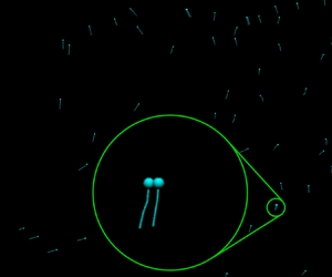
The experimental dataset presented in this paper was acquired in the same flow facility and particle tracking methodology specialized for small- $r$ measurements described in Hammond & Meng (Reference Hammond and Meng2021). As pictured in figure 1, we used a fan-driven, 1 m-diameter homogeneous isotropic turbulence (HIT) chamber, which produces isotropic turbulence with Taylor Reynolds number $Re_\lambda$ between 246 and 357 (Dou et al. Reference Dou, Pecenak, Cao, Woodward, Liang and Meng2016). The complete turbulence characteristics of this chamber are detailed in Dou et al. (Reference Dou, Pecenak, Cao, Woodward, Liang and Meng2016).

Figure 1. Schematic of the experimental measurement system used in the experiments (Hammond & Meng Reference Hammond and Meng2021).
To test the theory valid for  $St\ll 1$, we aimed to vary $St\lessapprox 1$ with constant $a$, and vary $a$ with constant $St<1$. To that end, we ran the flow facility at five different fan speeds which produced different turbulence strengths, and used four particle types with specifically chosen $a$ in the range of $3.75\,\mathrm {\mu }{\rm m}$– $20.75\,\mathrm {\mu }{\rm m}$, with different particle densities chosen to match $St$ at constant $a$. To acquire the particles, we used hollow spheres with different shell thicknesses (3M Glass Bubbles, types K25, S60 and IM16K) and specifically chosen diameters. The hollow spheres allowed particle size control through sieving and inertia control through choice of particle type (Dou et al. Reference Dou, Bragg, Hammond, Liang, Collins and Meng2018a,Reference Dou, Ireland, Bragg, Liang, Collins and Mengb). We sieved the originally widely polydisperse particles to acquire narrow size distributions for each of the four particle samples. Particle density was measured with a Micromeritics accu-Pyc II 1340 gas pycnometer. The flow and particle conditions of the experiments are listed in table 1. The condition at $St=0.74, a=14.25\,\mathrm {\mu }{\rm m}$ is identical to that reported in Hammond & Meng (Reference Hammond and Meng2021).
Table 1. Particle properties, Stokes numbers and corresponding flow conditions in the experiments. For complete flow details see Dou et al. (Reference Dou, Pecenak, Cao, Woodward, Liang and Meng2016).

The experimental set-up, matching that of Hammond & Meng (Reference Hammond and Meng2021), is shown in figure 1. Four high-speed pulsed lasers ( $2{\times }$ Photonics 30 mJ Nd-YLF, dual head, cross-polarized beams) fired four pulses in rapid succession and were directed and shaped into a 5 mm-thickness laser sheet in the centre of the HIT chamber. From the laser head, beam collimators at the apertures of lasers L1 and L2 kept the beam from expanding over the 6 m path to the flow facility. A 50/50 beam expander then combined the outputs of L1 and L2 such that all four pulses were mixed into two identical beam paths with 50 % of the pulse energy in each beam. Then, mirrors were used to direct the two identical beams to the flow facility centre. A quarter-wave plate converted the cross-polarized light to circularly polarized light to avoid imbalanced illumination due to the dependence of Mie scattering on polarization direction. A cylindrical lens was then used to spread the beam into a 5 mm-thickness sheet, and a square aperture provided sharp cutoffs of the illumination volume producing a $50\,{\rm mm} \times 30\,{\rm mm} \times 5\,{\rm mm}$ box illuminated by the four independently controllable laser pulses. The illuminated particles were then imaged by four high-speed cameras at four distinct points in time separated by $\Delta t_i$, where $i=1,2,3$. In these experiments, $\Delta t_1=\Delta t_3=1.6(\Delta t_2)$, where $\Delta t_2$ is given in table 1.
The imaging set-up, shown above the HIT chamber in figure 1, consisted of four Phantom Veo 640L cameras in frame-straddling mode with macro lenses on tilt mounts, mounted on a vibration isolating table. Vibration isolation was crucial in the experiments to avoid biases which may occur due to relative motion between cameras (Hammond & Meng Reference Hammond and Meng2021). The remaining vibration from the passive vibration-isolating table was a 3 Hz small-amplitude swaying of the entire table contents, which effectively caused an inconsequential change of the arbitrarily chosen coordinate origin of the experiment (Hammond & Meng Reference Hammond and Meng2021).
The experimental technique for  $g(r)$ measurement has been fully described in Hammond & Meng (Reference Hammond and Meng2021). Briefly, we used a four camera, three-dimensional particle tracking velocimetry system with a unique track interpolation approach to tackle small-separation measurement of particle positions. This was achieved using 4P-STB particle tracking (Novara et al. Reference Novara, Schanz, Geisler, Gesemann, Voss and Schroder2019) by LaVision (Göttingen, Germany), with the interpolated four-pulse track midpoint used as the particle position for calculation of $g(r)$. This method enabled the first-ever tracking of particle pairs in turbulence at extremely small separations where particle images would be overlapped and unrecoverable by traditional particle tracking algorithms. Measurements below this overlap limit were made possible by acquiring images of a near-contact particle pair just before and after they reach their closest approach.
Exploration into the potential biases of this measurement technique was performed in Hammond & Meng (Reference Hammond and Meng2021), and one potential bias intrinsic to all particle tracking velocimetry systems was identified and explored. Not all particles registered by the tracking system were actually tracked, in the case of these experiments, primarily due to the fluctuating intensity of particles caused by random fluctuations in local laser volumetric intensity arising from ambient dust in the laboratory occluding and interfering with the 6 m-long laser beam. It was identified that the particles lost by the tracking system were dispersed evenly through the flow volume, since motion of ambient dust is independent of the turbulence. Therefore, the track loss effectively resulted in a reduction of particle number density that does not affect  $g(r)$, since $g(r)$ is normalized based on number density. For a detailed description of the potential biases of experiments, please refer to Hammond & Meng (Reference Hammond and Meng2021).
Uncertainties in  $r$ and $g(r)$ were calculated following the method of Hammond & Meng (Reference Hammond and Meng2021) and are presented in Appendix B as error bars on the forthcoming experimental data. These two uncertainties had similar magnitudes across all conditions. Convergence of the r.d.f. was achieved and the standard error was ${<}2\,\%$. For statistical convergence, 15 465 realizations were acquired for the $a=14.25\,\mathrm {\mu }{\rm m}$ particles, and 9279 realizations for the other three types of particles.
3. Theory
3.1. Physical mechanism of HI-induced clustering
We begin by providing a physical explanation for how HI can lead to particle clustering in turbulence. As shown in Appendix A, the steady-state r.d.f.  $g(r)$ may be expressed exactly as
 \begin{equation} g(r)=\lim_{t\to\infty}\left\langle\exp\left(-\int^t_0\boldsymbol{\nabla}\boldsymbol{\cdot} \boldsymbol{\mathcal{W}}(\boldsymbol{\xi}(s),s)\,{\rm d}s\right)\right\rangle_{{r}}, \end{equation}
where  $\boldsymbol {\mathcal {W}}$ is the relative velocity field between two particles which is formally defined as
 \begin{equation} \boldsymbol{\mathcal{W}}(\boldsymbol{r},t)\equiv \left\langle\boldsymbol{w}^p(t)\right\rangle^{\boldsymbol{r}^p(0),\boldsymbol{w}^p(0)}_{\boldsymbol{r},\boldsymbol{u}}, \end{equation}
where  $\boldsymbol {w}^p(t)$ is the relative velocity between two particles with separation $\boldsymbol {r}^p(t)$, and the operator $\langle \cdot \rangle ^{\boldsymbol {r}^p(0),\boldsymbol {w}^p(0)}_{\boldsymbol {r},\boldsymbol {u}}$ denotes an ensemble average over all initial particle-pair separations $\boldsymbol {r}^p(0)$ and initial relative velocities $\boldsymbol {w}^p(0)$, conditioned on a given realization of the flow $\boldsymbol {u}$, and conditioned on $\boldsymbol {r}^p(t)=\boldsymbol {r}$. This field reduces to $\boldsymbol {\mathcal {W}}(\boldsymbol {r},t)= \boldsymbol {w}^p(t\vert \boldsymbol {r})$ in the limit where there is a unique initial condition that generates a trajectory satisfying $\boldsymbol {r}^p(t)=\boldsymbol {r}$, such as is the case for fluid particles or $St\ll 1$. The characteristic variable $\boldsymbol {\xi }$ is defined via $\partial _s\boldsymbol {\xi }\equiv \boldsymbol{\mathcal {W}}(\boldsymbol {\xi }(s),s)$, and $\langle \cdot \rangle _{{r}}$ denotes an ensemble average conditioned on the particles having the separation $\|\boldsymbol {\xi }(t)\|={r}$. For fluid particles, $\boldsymbol {\nabla }\boldsymbol {\cdot }\boldsymbol {\mathcal {W}}=0$ in an incompressible flow and so $g(r)=1$, i.e. they do not cluster. However, if $\boldsymbol {\nabla }\boldsymbol {\cdot }\boldsymbol {\mathcal {W}}$ is finite, clustering may occur with $g(r)>1$.
If we consider monodisperse particle pairs with radius  $a$ that experience HI, then for $St\to 0$ we have $\boldsymbol {\nabla }\boldsymbol {\cdot }\boldsymbol {\mathcal {W}}=\lambda \mathcal {S}_{\parallel }$ (Brunk et al. Reference Brunk, Koch and Lion1997), where $\lambda \geq 0$ is a non-dimensional, nonlinear function of $r/a$ that characterizes the HI, and $\mathcal {S}_{\parallel }$ is the fluid strain rate parallel to the particle-pair separation vector. Since $\lambda \geq 0$, then the particle field will be compressed in regions where $\mathcal {S}_{\parallel }<0$, and dilated in regions where $\mathcal {S}_{\parallel }>0$. That $\boldsymbol {\nabla }\boldsymbol {\cdot }\boldsymbol {\mathcal {W}}\neq 0$ is due to the disturbance fields in the flow produced by displacement of the fluid around the two particles, which in turn generates forces on the particles. This force either causes the particles to be attracted or repelled from each other, and vanishes for fluid particles ( $a=0$) since they do not disturb the flow.
Using  $\boldsymbol {\nabla }\boldsymbol {\cdot }\boldsymbol {\mathcal {W}}=\lambda \mathcal {S}_{\parallel }$ in (3.1) we see that $g(r)>1$ is associated with a preference for trajectories with $\int ^t_0 \lambda (\xi (s))\mathcal {S}_{\parallel }(s)\,{\rm d}s<0$, that arises precisely because the particles are compressed into regions where $\mathcal {S}_{\parallel }<0$. This phenomenon is similar to the case of inertial particles with $St\ll 1$ (without HI) whose clustering is driven by preferential sampling of weak-vorticity, high-strain regions of the flow (Chun et al. Reference Chun, Koch, Rani, Ahluwalia and Collins2005; Bragg & Collins Reference Bragg and Collins2014; Bragg, Ireland & Collins Reference Bragg, Ireland and Collins2015), that arises due to the particles being centrifuged out of vortical regions of the flow (Maxey Reference Maxey1987).
The HI effect on clustering is dependent on  $St$. Since HI only occur when $r$ is sufficiently small, we define $\ell _a$ as the length scale of the hydrodynamic disturbance, below which HI become appreciable. At $r>\ell _a$, HI are not important, and the clustering arises solely due to how inertia modifies the particle interaction with the turbulence (Bragg & Collins Reference Bragg and Collins2014; Bragg et al. Reference Bragg, Ireland and Collins2015). For $r<\ell _a$ and $St\ll 1$, the physical mechanism leading to r.d.f. enhancement comes from particles being compressed into regions where $\mathcal {S}_{\parallel }<0$ as discussed above, with sub-leading corrections to the trajectories due to inertia. For $r<\ell _a$ and $St\geq O(1)$, the mechanism generating $g(r\leq \ell _a)>1$ will be strongly affected by the non-local dependence of $\boldsymbol {\mathcal {W}}(\boldsymbol {\xi }(s),s)$ upon the turbulence the particles have experienced along their path-history at times $s'< s$ (Bragg & Collins Reference Bragg and Collins2014; Bragg et al. Reference Bragg, Ireland and Collins2015).
3.2. Theory for the r.d.f. assuming  $St\ll 1$

While (3.1) is useful for understanding how particles cluster, it is not straightforward to derive from this a closed expression for  $g(r)$. Yavuz et al. (Reference Yavuz, Kunnen, van Heijst and Clercx2018) developed a theoretical model for $g(r)$ in the regime $St\ll 1$, based on the drift-diffusion models of Brunk et al. (Reference Brunk, Koch and Lion1997) and Chun et al. (Reference Chun, Koch, Rani, Ahluwalia and Collins2005). However, in going through their analysis we have found several significant errors. Therefore, in the following, we re-derive the correct form of the theory and discuss the differences with the result in Yavuz et al. (Reference Yavuz, Kunnen, van Heijst and Clercx2018).
Following Chun et al. (Reference Chun, Koch, Rani, Ahluwalia and Collins2005), Yavuz et al. (Reference Yavuz, Kunnen, van Heijst and Clercx2018) consider the transport equation governing the probability density function (p.d.f.)  $\rho (\boldsymbol {r},t)\equiv \langle \delta (\boldsymbol {r}^p(t)-\boldsymbol {r})\rangle$ (that will eventually be related to the r.d.f.) which at steady state is
 $$\begin{gather} \frac{\partial}{\partial\boldsymbol{r}}\boldsymbol{\cdot}\left(\boldsymbol{q}^{D}+ \boldsymbol{q}^{d}\right)={0}, \end{gather}$$
 $$\begin{gather}\boldsymbol{q}^{D}(\boldsymbol{r})\approx{-}B^{nl}\int_{-\infty}^0\left\langle\boldsymbol{\mathcal{W}}(\boldsymbol{r},0)\boldsymbol{\mathcal{W}}(\boldsymbol{r},s)\right\rangle\,{\rm d}s \boldsymbol{\cdot}\frac{\partial}{\partial\boldsymbol{r}}\rho(\boldsymbol{r})\,{\rm d}s, \end{gather}$$
 $$\begin{gather}\boldsymbol{q}^{d}(\boldsymbol{r})\approx{-}\rho(\boldsymbol{r})\int_{-\infty}^0 \left\langle\boldsymbol{\mathcal{W}}(\boldsymbol{r},0)\frac{\partial}{\partial\boldsymbol{r}}\boldsymbol{\cdot} \boldsymbol{\mathcal{W}}(\boldsymbol{r},s) \right\rangle\,{\rm d}s, \end{gather}$$
where  $\boldsymbol {q}^{D}$ and $\boldsymbol {q}^{d}$ are the diffusion and drift vectors, respectively. The expressions for $\boldsymbol {q}^{D}$ and $\boldsymbol {q}^{d}$ stated above are approximate because they have been developed under the diffusion approximation discussed in Brunk et al. (Reference Brunk, Koch and Lion1997) and Chun et al. (Reference Chun, Koch, Rani, Ahluwalia and Collins2005), wherein it is assumed that over the correlation time of the local flow field, the change in the particle-pair separation is small compared with their separation. As discussed in Chun et al. (Reference Chun, Koch, Rani, Ahluwalia and Collins2005), the diffusion approximation is not valid in real turbulence since the correlation time of the flow is of the same order as that on which the particle-pair separation evolves. Nevertheless, in Chun et al. (Reference Chun, Koch, Rani, Ahluwalia and Collins2005) it is argued that in real turbulence, the diffusion approximation gives the correct functional forms in the model, and the quantitative error associated with the diffusion approximation can be corrected for using a ‘non-local’ correction coefficient, denoted by $B^{nl}$ in the above expression for $\boldsymbol {q}^{D}$.
To construct a solution for  $\rho (\boldsymbol {r})$ using (3.3) for the regime $St\ll 1$, the correlations in $\boldsymbol {q}^{D}$ and $\boldsymbol {q}^{d}$ involving the particle velocity field $\boldsymbol {\mathcal {W}}$ must be specified, and these are constructed using solutions to the particle equation of motion in the regime $St\ll 1$. For this Yavuz et al. (Reference Yavuz, Kunnen, van Heijst and Clercx2018) consider monodisperse pairs of small, heavy, inertial particles subject to HI in steady Stokes flow, whose equation of relative motion is
 \begin{equation} \boldsymbol{w}^p(t)=St\tau_\eta\boldsymbol{J}^p\boldsymbol{\cdot}\dot{\boldsymbol{w}}^p+\boldsymbol{f}^p+St\tau_\eta\frac{3a}{5\|\boldsymbol{r}^p\|}C\boldsymbol{\dot{\varUpsilon}}^p\times\boldsymbol{r}^p,\end{equation}
where  $\boldsymbol {r}^p(t),\boldsymbol {w}^p(t)$ are the particle-pair relative separation and relative velocity, (the relative velocity $\boldsymbol {w}^p(t)$ is simply the difference between the velocity of the two particles, and in general differs from the relative velocity field $\boldsymbol {\mathcal {W}}$ defined in (3.2). However, for $St\ll 1$, $\boldsymbol {w}^p(t\vert \boldsymbol {r}^p(t)=\boldsymbol {r})=\boldsymbol {\mathcal {W}}(\boldsymbol {r},t)+O(St)$) respectively, $\boldsymbol {\varUpsilon }^p$ is the sum of the angular velocities of the two particles, $\boldsymbol {J}^p=\boldsymbol {J}(\boldsymbol {r}^p(t))$, $\boldsymbol {f}^p=\boldsymbol {f}(\boldsymbol {x}^p(t),\boldsymbol {r}^p(t),t)$, with
 $$\begin{gather} \boldsymbol{J}(\boldsymbol{r})\equiv\left(A\frac{\boldsymbol{r}\boldsymbol{r}}{\|\boldsymbol{r}\|^2} +B\left[\boldsymbol{I}-\frac{\boldsymbol{r}\boldsymbol{r}}{\|\boldsymbol{r}\|^2}\right] \right), \end{gather}$$
 $$\begin{gather}\boldsymbol{f}(\boldsymbol{x},\boldsymbol{r},t)\equiv\boldsymbol{\varGamma}\boldsymbol{\cdot} \boldsymbol{r}-2a\left(D\frac{\boldsymbol{r}\boldsymbol{r}}{\|\boldsymbol{r}\|^2} +E\left[\boldsymbol{I}-\frac{\boldsymbol{r}\boldsymbol{r}}{\|\boldsymbol{r}\|^2}\right] \right)\boldsymbol{\cdot}\frac{(\boldsymbol{S}\boldsymbol{\cdot} \boldsymbol{r})}{\|\boldsymbol{r}\|}, \end{gather}$$
where  $\boldsymbol {x}^p(t)$ is the position of the primary particle (relative to which the motion of the satellite particle is considered), and where $\boldsymbol {x}$ refers to the arguments of the velocity gradient $\boldsymbol {\varGamma }(\boldsymbol {x},t)\equiv \boldsymbol {\nabla } \boldsymbol {u}$ and the strain rate $\boldsymbol {S}(\boldsymbol {x},t)\equiv ( \boldsymbol {\nabla } \boldsymbol {u}+ \boldsymbol {\nabla } \boldsymbol {u}^\top )/2$. The terms $A,B,C,D,E$ are non-dimensional functions of $r/a\equiv \|\boldsymbol {r}\|/a$ only, whose forms may be found in Kim & Karrila (Reference Kim and Karrila1991).
Yavuz et al. (Reference Yavuz, Kunnen, van Heijst and Clercx2018) then expand (3.6) in  $St$ so that to order $O(St^2)$ we obtain
 \begin{equation} \boldsymbol{w}^p(t)=St\tau_\eta\boldsymbol{J}^p\boldsymbol{\cdot}\frac{{\rm d}}{{\rm d}t}\boldsymbol{f}^p+\boldsymbol{f}^p+St\tau_\eta\frac{3a}{5\|\boldsymbol{r}^p\|}C\boldsymbol{\dot{\varUpsilon}}^p\times\boldsymbol{ r}^p+O(St^2), \end{equation}
and based on the definition of the field  $\boldsymbol {\mathcal {W}}$ in (3.2) this leads to
 \begin{equation} {\boldsymbol{\mathcal{W}}}=St\tau_\eta\boldsymbol{J}\boldsymbol{\cdot}\frac{{\rm D}}{{\rm D}t}\boldsymbol{f}+\boldsymbol{f}+St\tau_\eta\frac{3a}{5 r}C\dot{\boldsymbol{\varTheta}}\times\boldsymbol{r}+O(St^2),\end{equation}
where
 \begin{equation} \dot{\boldsymbol{{\varTheta}}}(\boldsymbol{r},t)\equiv \left\langle\boldsymbol{\dot{\varUpsilon}}^p\right\rangle^{\boldsymbol{r}^p(0),\boldsymbol{w}^p(0)}_{\boldsymbol{r},\boldsymbol{u}}. \end{equation}
 Note that, owing to the definition of  $\boldsymbol {\mathcal {W}}$, in (3.10) the term $\boldsymbol {f}$ is explicitly $\boldsymbol {f}(\boldsymbol {x}^p(t),\boldsymbol {r},t)$, i.e. $\boldsymbol {f}$ measured at fixed separation $\boldsymbol {r}$, but along the time-dependent reference particle trajectory $\boldsymbol {x}^p(t)$.
For clarity, we now switch to index notation, and write the result for  ${\boldsymbol {\mathcal {W}}}$ in the form of an expansion in $St$
$St$
 $$\begin{gather} \mathcal{W}_i= \mathcal{W}_i^{[0]}+St \mathcal{W}_i^{[1]}+O(St^2), \end{gather}$$
 $$\begin{gather}\mathcal{W}_i^{[0]}\equiv f_i, \end{gather}$$
 $$\begin{gather}\mathcal{W}_i^{[1]}\equiv \tau_\eta J_{ij} \frac{{\rm D}}{{\rm D}t}f_j+\tau_\eta\frac{3a}{5 r}C\epsilon_{ijk}\dot{\varTheta}_j r_k, \end{gather}$$
so that, to leading order in  $St$, the diffusion velocity is
 \begin{equation} {q}_i^D(\boldsymbol{r})={-}B^{nl}\int_{-\infty}^0 \left\langle\mathcal{W}^{[0]}_i(\boldsymbol{r},0)\mathcal{W}^{[0]}_j(\boldsymbol{r},s)\right\rangle\,{\rm d}s \frac{\partial}{\partial r_j}\rho, \end{equation}
while the drift velocity is to  $O(St^2)$
 \begin{align} {q}_i^d(\boldsymbol{r})&={-}\rho\int_{-\infty}^0 \left\langle\mathcal{W}^{[0]}_i(\boldsymbol{r},0)\frac{\partial}{\partial r_l}{\mathcal{W}}^{[0]}_l(\boldsymbol{r},s)\right\rangle\,{\rm d}s\nonumber\\ &\quad-St \rho\int_{-\infty}^0 \left\langle\mathcal{W}^{[0]}_i(\boldsymbol{r},0)\frac{\partial}{\partial r_l}{\mathcal{W}}^{[1]}_l(\boldsymbol{r},s)\right\rangle\,{\rm d}s\nonumber\\ &\quad-St \rho\int_{-\infty}^0 \left\langle\mathcal{W}^{[1]}_i(\boldsymbol{r},0)\frac{\partial}{\partial r_l}{\mathcal{W}}^{[0]}_l(\boldsymbol{r},s)\right\rangle\,{\rm d}s\nonumber\\ &\quad-St^2 \rho\int_{-\infty}^0\left\langle \mathcal{W}^{[1]}_i(\boldsymbol{r},0)\frac{\partial}{\partial r_l}{\mathcal{W}}^{[1]}_l(\boldsymbol{r},s)\right\rangle\,{\rm d}s. \end{align}
Yavuz et al. (Reference Yavuz, Kunnen, van Heijst and Clercx2018) then focus on the far-field asymptotic behaviour where  $a/r\ll 1$, retaining at each order in $St$ only the leading-order contributions from HI. In order to obtain these, we must use the far-field forms of $\boldsymbol {f}$ and $\boldsymbol {J}$, which are obtained using the far-field asymptotic relations $A(r)\sim -1+3a/2r$, $B(r)\sim -1+3a/4r$, $D(r)\sim 5a^2/2 r^2 - 4 a^4/r^4 + 25 a^5/2 r^5$, $E(r)\sim 8 a^4/3r^4$ (Batchelor & Green Reference Batchelor and Green1972; Kim & Karrila Reference Kim and Karrila1991).
The required far-field forms are then
 $$\begin{gather} \mathcal{W}_i^{[0]}(\boldsymbol{r},t)\sim \varGamma^f_{ij}r_j, \end{gather}$$
 $$\begin{gather}\frac{\partial}{\partial r_l}{\mathcal{W}}^{[0]}_l(\boldsymbol{r},t)\sim 75\frac{a^6}{r^6}S^f_{kn}\frac{r_k r_n}{r^2}, \end{gather}$$
 $$\begin{gather}\mathcal{W}^{[1]}_i(\boldsymbol{r},t)\sim \tau_\eta\left(\frac{3a}{4r}-1\right)\varGamma_{ik}^f\varGamma^f_{km}r_m+\tau_\eta \frac{3a}{4r}\frac{r_i r_j r_m}{r^2} \varGamma_{jk}^f\varGamma^f_{km}, \end{gather}$$
 $$\begin{gather}\frac{\partial}{\partial r_l}{\mathcal{W}}^{[1]}_l(\boldsymbol{r},t)\sim\tau_\eta \left(\frac{3a}{4r}-1\right)\varGamma^f_{nm}\varGamma^f_{mn}+\tau_\eta\frac{3a}{4r}\frac{r_j r_n}{r^2}\varGamma^f_{jm}\varGamma^f_{mn}. \end{gather}$$
In these expressions we have used the assumption that  $\boldsymbol {\varGamma }$ along the particle trajectory $\boldsymbol {x}^p(t)$ can be replaced by that along the trajectory of an inertialess particle $\boldsymbol {x}^f(t)$, so that the above results contain $\boldsymbol {\varGamma }^f(t)\equiv \boldsymbol {\varGamma }(\boldsymbol {x}^f(t),t)$ and $\boldsymbol {S}^f(t)\equiv \boldsymbol {S}(\boldsymbol {x}^f(t),t)$. This is the same assumption made in Chun et al. (Reference Chun, Koch, Rani, Ahluwalia and Collins2005), upon which this present model is based, and as argued in Chun et al. (Reference Chun, Koch, Rani, Ahluwalia and Collins2005), it is reasonable for $St\ll 1$. One difference, however, is that in the present model, the inertialess particle trajectory $\boldsymbol {x}^f(t)$ cannot be interpreted as that of a fluid particle due to the influence of HI on the particle trajectory. In the above results we have also thrown away the terms involving $\dot {\boldsymbol {{\varTheta }}}$, since as noted in Yavuz et al. (Reference Yavuz, Kunnen, van Heijst and Clercx2018), this term is sub-leading in the far field under the assumptions $St\ll 1$ and that the local flow around the particles is steady Stokes flow.
Concerning the diffusion term, using the far-field result in (3.17) and invoking isotropy yields to leading order in  $St$ (Yavuz et al. Reference Yavuz, Kunnen, van Heijst and Clercx2018)
 \begin{equation} q^D_{i}(\boldsymbol{r})\sim{-} B^{nl}r r_i\tau_\eta^{{-}1} \boldsymbol{\nabla}\rho. \end{equation}
This is the same diffusion coefficient as in Chun et al. (Reference Chun, Koch, Rani, Ahluwalia and Collins2005), reflecting the fact that HI does not make a leading-order contribution to the diffusion process.
Assuming isotropy of the flow, the far-field form of the first contribution in (3.16), which is  $O(St^0)$, is
 \begin{equation} \int_{-\infty}^0 \left\langle\mathcal{W}^{[0]}_i(\boldsymbol{r},0)\frac{\partial}{\partial r_l}{\mathcal{W}}^{[0]}_l(\boldsymbol{r},s)\right\rangle\,{\rm d}s \sim 10\frac{a^6}{r^6}\tau_S r_i \langle S^2\rangle, \end{equation}
where  $\tau _S$ is the correlation time scale of the strain rate $\boldsymbol {S}^f$, and $\langle S^2\rangle \equiv \langle S^f_{ab}(0)S^f_{ab}(0)\rangle$. This result is the same as the far-field version of the drift velocity derived in Brunk et al. (Reference Brunk, Koch and Lion1997) and is also the leading-order contribution to $\boldsymbol {q}^d$ derived in Yavuz et al. (Reference Yavuz, Kunnen, van Heijst and Clercx2018). The results presented so far match exactly those in Yavuz et al. (Reference Yavuz, Kunnen, van Heijst and Clercx2018). However, we found several issues with their handling of the other contributions to the drift term $\boldsymbol {q}^d$ which we now discuss.
In Yavuz et al. (Reference Yavuz, Kunnen, van Heijst and Clercx2018), it is argued that the  $O(St)$ contributions to $\boldsymbol {q}^d$ disappear due to isotropy of the flow, and we now investigate this claim. In the far field, the second contribution in (3.16), which is $O(St)$, involves
 $$\begin{gather} \int_{-\infty}^0 \left\langle\mathcal{W}^{[0]}_i(\boldsymbol{r},0)\frac{\partial}{\partial r_l}{\mathcal{W}}^{[1]}_l(\boldsymbol{r},s)\right\rangle\,{\rm d}s\sim \tau_\eta \left(\frac{3a}{4r}-1\right)r_j \int_{-\infty}^0 \left\langle\varGamma^f_{ij}(0) \varGamma^f_{nm}(s)\varGamma^f_{mn}(s)\right\rangle\,{\rm d}s\nonumber\\ +\tau_\eta \frac{3a}{4r}\frac{r_j r_k r_n}{r^2} \int_{-\infty}^0 \left\langle\varGamma^f_{ij}(0)\varGamma^f_{km}(s)\varGamma^f_{mn}(s)\right\rangle\,{\rm d}s. \end{gather}$$
Invoking isotropy, incompressibility we have
 \begin{equation} \left\langle\varGamma^f_{ij}(0)\varGamma^f_{nm}(t)\varGamma^f_{mn}(t)\right\rangle=\frac{\delta_{ij}}{3}\left\langle\varGamma^f_{aa}(0)\varGamma^f_{nm}(s)\varGamma^f_{mn}(s) \right\rangle=0, \end{equation}
and
 \begin{equation} \left\langle\varGamma^f_{ij}(0)\varGamma^f_{km}(s)\varGamma^f_{mn}(s)\right\rangle=\frac{1}{30} \left\langle\varGamma^f_{bc}(0)\varGamma^f_{bd}(s)\varGamma^f_{dc}(s)\right\rangle\left(4\delta_{ik}\delta_{jn}-\delta_{ij}\delta_{kn} -\delta_{in}\delta_{jk} \right). \end{equation}
Yavuz et al. (Reference Yavuz, Kunnen, van Heijst and Clercx2018) correctly identified the correlation in (3.24) as being zero, but assumed that the correlation in (3.25) is also zero. The correlation in (3.25) may be written as
 \begin{equation} \left\langle\varGamma^f_{bc}(0)\varGamma^f_{bd}(s)\varGamma^f_{dc}(s)\right\rangle=\left\langle\varGamma^f_{bc}(0)\varGamma^f_{bd}(0)\varGamma^f_{dc}(0)\right\rangle\varSigma(s), \end{equation}
where  $\varSigma$ denotes the autocorrelation for the quantity, and by introducing the strain rate $\boldsymbol {S}$ and vorticity $\boldsymbol {\varOmega }$, the single-time invariant can be written as
 \begin{equation} \left\langle\varGamma^f_{bc}(0)\varGamma^f_{bd}(0)\varGamma^f_{dc}(0)\right\rangle=\left\langle{S}^f_{bc}(0){S}^f_{bd}(0){S}^f_{dc}(0)\right\rangle-\frac{1}{4}\left\langle{S}^f_{bc}(0)\varOmega^f_{b}(0)\varOmega^f_{c}(0)\right\rangle. \end{equation}
This invariant is not zero; the first term on the right-hand side is the strain-rate production term which is negative, and the second is the enstrophy production term (Tsinober Reference Tsinober2001). These invariants are finite in three-dimensional turbulence, and are directly connected to the energy cascade process (Carbone & Bragg Reference Carbone and Bragg2020; Johnson Reference Johnson2020). Thus, interestingly, the processes governing the energy cascade also contribute to inertial particle clustering in the presence of HI.
Using the results above in (3.23) we obtain
 \begin{equation} \int_{-\infty}^0 \left\langle\mathcal{W}^{[0]}_i(\boldsymbol{r},0)\frac{\partial}{\partial r_l}{\mathcal{W}}^{[1]}_l(\boldsymbol{r},s)\right\rangle\,{\rm d}s\sim\frac{a \tau_\eta \tau_{\varSigma}}{20 r}r_i\langle \varGamma^3\rangle, \end{equation}
where  $\tau _{\varSigma }$ is the time scale associated with the autocorrelation $\varSigma$, and $\langle \varGamma ^3\rangle \equiv \langle \varGamma ^f_{bc}(0)\varGamma ^f_{bd}(0)\varGamma ^f_{dc}(0)\rangle$. Note that, since $\langle \varGamma ^3\rangle <0$ in three-dimensional turbulence (Tsinober Reference Tsinober2001), then (3.28) makes a positive contribution to the drift velocity $\boldsymbol {q}^d$ and therefore actually opposes the clustering of the particles.
In the far field, the third contribution in (3.16), which is  $O(St)$, involves
 $$\begin{gather} \int_{-\infty}^0\left\langle \mathcal{W}^{[1]}_i(\boldsymbol{r},0)\frac{\partial}{\partial r_l}{\mathcal{W}}^{[0]}_l(\boldsymbol{r},s)\right\rangle\,{\rm d}s\sim75\frac{ a^6}{r^6}\tau_\eta\frac{r_m r_l r_q}{r^2}\left(\frac{3a}{4r}-1\right)\int_{-\infty}^0 \left\langle\varGamma^f_{ik}(0)\varGamma^f_{km}(0)S^f_{lq}(s)\right\rangle\,{\rm d}s\nonumber\\ +\frac{225}{4}\frac{ a^7}{r^7}\tau_\eta\frac{r_i r_j r_m r_l r_q}{r^4}\int_{-\infty}^0 \left\langle\varGamma^f_{jk}(0)\varGamma^f_{km}(0)S^f_{lq}(s)\right\rangle\,{\rm d}s. \end{gather}$$
Similar to before, invoking isotropy we have
 \begin{equation} \left\langle\varGamma^f_{ik}(0)\varGamma^f_{km}(0)S^f_{lq}(s)\right\rangle=\frac{1}{60} \left\langle\varGamma^f_{bc}(0)\varGamma^f_{cd}(0)\varGamma^f_{bd}(0)\right\rangle\left(4\delta_{il}\delta_{mq}-\delta_{im}\delta_{lq} -\delta_{iq}\delta_{ml} \right) \varSigma'(s), \end{equation}
where  $\varSigma '$ denotes the autocorrelation for the quantity, and we have used the results of Betchov (Reference Betchov1956) to obtain
 \begin{equation} \left\langle\varGamma^f_{bc}(0)\varGamma^f_{cd}(0)S^f_{bd}(0)\right\rangle=\frac{1}{2}\left\langle\varGamma^f_{bc}(0)\varGamma^f_{cd}(0)\varGamma^f_{bd}(0)\right\rangle. \end{equation}
Putting this all together we obtain
 \begin{equation} \int_{-\infty}^0 \left\langle\mathcal{W}^{[1]}_i(\boldsymbol{r},0)\frac{\partial}{\partial r_l}{\mathcal{W}}^{[0]}_l(\boldsymbol{r},s)\right\rangle\,{\rm d}s\sim\frac{5}{2}\left(\frac{3 a}{2r}-1 \right)\frac{a^6}{r^6}\tau_\eta\tau_{\varSigma'} r_i\langle \varGamma^3\rangle,\end{equation}
where  $\tau _{\varSigma '}$ is the time scale associated with the autocorrelation $\varSigma '$.
In the far field, the fourth contribution in (3.16), which is  $O(St^2)$, involves
 \begin{align} &\int_{-\infty}^0 \left\langle\mathcal{W}^{[1]}_i(\boldsymbol{r},0)\frac{\partial}{\partial r_l}{\mathcal{W}}^{[1]}_l(\boldsymbol{r},s)\right\rangle\,{\rm d}s\nonumber\\ &\quad\sim \tau_\eta^2\left(\frac{3a}{4 r}-1\right)^2 r_m \int_{-\infty}^0 \left\langle\varGamma^f_{ik}(0)\varGamma^f_{km}(0)\varGamma^f_{np}(s)\varGamma^f_{pn}(s) \right\rangle\,{\rm d}s\nonumber\\ &\qquad+\tau_\eta^2\frac{3a}{4 r}\left(\frac{3a}{4 r}-1\right) \frac{r_m r_j r_n}{r^2} \int_{-\infty}^0 \left\langle\varGamma^f_{ik}(0)\varGamma^f_{km}(0)\varGamma^f_{jp}(s)\varGamma^f_{pn}(s) \right\rangle\,{\rm d}s\nonumber\\ &\qquad+\tau_\eta^2\frac{3a}{4 r}\left(\frac{3a}{4 r}-1\right) \frac{r_i r_j r_m}{r^2} \int_{-\infty}^0 \left\langle\varGamma^f_{jk}(0)\varGamma^f_{km}(0)\varGamma^f_{np}(s)\varGamma^f_{pn}(s) \right\rangle\,{\rm d}s\nonumber\\ &\qquad+\tau_\eta^2\left(\frac{3a}{4 r}\right)^2 \frac{r_i r_j r_m r_p r_q}{r^4} \int_{-\infty}^0 \left\langle\varGamma^f_{jk}(0)\varGamma^f_{km}(0)\varGamma^f_{pl}(s)\varGamma^f_{lq}(s) \right\rangle\,{\rm d}s. \end{align}
These integrals involve the quantity (with differing index labels)
 \begin{equation} A_{imjn}(s)\equiv\left\langle\varGamma^f_{ik}(0)\varGamma^f_{km}(0)\varGamma^f_{jp}(s)\varGamma^f_{pn}(s) \right\rangle, \end{equation}
and this may be re-written using isotropy and autocorrelation functions as
 \begin{align} A_{imjn}(s)&=\frac{\langle \varGamma^4_1\rangle}{30}\left(4\delta_{im}\delta_{jn}-\delta_{ij}\delta_{mn}-\delta_{in}\delta_{mj}\right)\varPsi_1(s)\nonumber\\ &\quad+\frac{\langle \varGamma^4_2\rangle}{30}\left(-\delta_{im}\delta_{jn}+4\delta_{ij}\delta_{mn}-\delta_{in}\delta_{mj}\right)\varPsi_2(s)\nonumber\\ &\quad+\frac{\langle \varGamma^4_2\rangle}{30}\left(-\delta_{im}\delta_{jn}-\delta_{ij}\delta_{mn}+4\delta_{in}\delta_{mj}\right)\varPsi_3(s), \end{align}
where  $\langle \varGamma ^4_1\rangle \equiv A_{aabb}(0)$, $\langle \varGamma ^4_2\rangle \equiv A_{abab}(0)$, $\langle \varGamma ^4_3\rangle \equiv A_{abba}(0)$. Using this in (3.33) we obtain
 $$\begin{gather} \int_{-\infty}^0 \left\langle\mathcal{W}^{[1]}_i(\boldsymbol{r},0)\frac{\partial}{\partial r_l}{\mathcal{W}}^{[1]}_l(\boldsymbol{r},s)\right\rangle\,{\rm d}s \sim \tau_\eta^2\tau_{\varPsi_1}\frac{\langle \varGamma^4_1\rangle}{3}r_i\left(\frac{3a}{4 r}-1\right)\left(\frac{3a}{2r}-1\right)\nonumber\\ +\frac{2}{15}\left(\left(\frac{3a}{4 r}\right)^2-\frac{3a}{8 r}\right)\tau_\eta^2r_i\left(\langle \varGamma^4_1\rangle\tau_{\varPsi_1}+\langle \varGamma^4_2\rangle\tau_{\varPsi_2}+\langle \varGamma^4_3\rangle\tau_{\varPsi_3} \right), \end{gather}$$
where  $\tau _{\varPsi _1}, \tau _{\varPsi _2}, \tau _{\varPsi _3}$ are the time scales associated with $\varPsi _1(s),\varPsi _2(s),\varPsi _3(s)$. This is essentially the same as the result Yavuz et al. (Reference Yavuz, Kunnen, van Heijst and Clercx2018) obtain for the $O(St^2)$ contribution to $\boldsymbol {q}^d$ except that we chose to express $A_{imjn}$ in terms of its basic invariants, whereas Yavuz et al. (Reference Yavuz, Kunnen, van Heijst and Clercx2018) wrote it in terms of its components in particular coordinate directions.
We now gather together all the contributions to (3.16) and substitute this along with (3.21) into (3.3), and use (A2) to obtain the following solution for the r.d.f.
 \begin{equation} g(r)\sim \left(\frac{r}{a}\right)^{{-}St^2\mu_4}\exp\left( \mu_1\left(\frac{r}{a}\right)^{{-}6}+(St\mu_2 +St^2\mu_3)\left(\frac{r}{a}\right)^{{-}1}\right),\end{equation}
where
 $$\begin{gather} \mu_1\equiv 5\tau_\eta\tau_S\langle S^2\rangle/3B^{nl}, \end{gather}$$
 $$\begin{gather}\mu_2\equiv \tau_\eta^2\tau_\varSigma\langle\varGamma^3\rangle/20B^{nl}, \end{gather}$$
 $$\begin{gather}\mu_3 \equiv{-}9\tau_\eta^3\tau_{\varPsi_1}\langle \varGamma^4_1\rangle/12 B^{nl}-\tau_\eta^3\left(\langle \varGamma^4_1\rangle\tau_{\varPsi_1}+\langle \varGamma^4_2\rangle\tau_{\varPsi_2}+\langle \varGamma^4_3\rangle\tau_{\varPsi_3} \right)/20 B^{nl}, \end{gather}$$
 $$\begin{gather}\mu_4\equiv \tau_\eta^3 \tau_{\varPsi_1}\langle \varGamma^4_1\rangle/3 B^{nl}. \end{gather}$$
Note that, in (3.37), at each order in  $St$, only the leading-order contribution in $a/r$ has been retained, which is why the contribution from (3.32) (which gives a contribution to the r.d.f. of $O(St[r/a]^{-6}])$) has disappeared.
Two of the four terms in (3.37) have been characterized in the literature previously. In the absence of HI,  ${\mu _1=\mu _2=\mu _3=0}$, and $g(r)\sim (r/a)^{- St^2\mu _4}$ describes the clustering in turbulence due solely to particle inertia (Chun et al. Reference Chun, Koch, Rani, Ahluwalia and Collins2005). The leading HI contribution $\exp ( \mu _1 a^6/r^6)$ is the far-field form of the result derived in Brunk et al. (Reference Brunk, Koch and Lion1997), which is independent of $St$ and describes the clustering due to HI that can occur even for $St=0$.
The  $O (St^2)$ inertial contribution to the clustering arising from HI, $\exp (St^2 \mu _3 a/r)$, was first derived in Yavuz et al. (Reference Yavuz, Kunnen, van Heijst and Clercx2018). They determined $\mu _3$ by fitting $\exp (St^2 \mu _3 a/r)$ to their experimental data, obtaining $\mu _3> 0$. From their definitions it follows trivially that $\langle \varGamma ^4_1\rangle \geq 0,\langle \varGamma ^4_2\rangle \geq 0$. The quantity $\langle \varGamma ^4_3\rangle$ is the average of the invariant $\varGamma ^f_{ak}(0)\varGamma ^f_{kb}(0)\varGamma ^f_{bp}(0)\varGamma ^f_{pa}(0)$, and using the Cayley–Hamilton theorem we can derive the result
 \begin{equation} \varGamma^f_{ak}(0)\varGamma^f_{kb}(0)\varGamma^f_{bp}(0)\varGamma^f_{pa}(0)=(1/2) \left( \varGamma^f_{cd}(0)\varGamma^f_{dc}(0)\right)^2, \end{equation}
and hence  $\langle \varGamma ^4_3\rangle \geq 0$. In view of this, and the non-negativity of $B_{nl}$ and $\tau _\eta$, it follows that provided the time scales $\tau _{\varPsi _1},\tau _{\varPsi _2},\tau _{\varPsi _3}$ are non-negative (which seems very reasonable to assume), then the theory dictates that $\mu _3\leq 0$. This then calls into question the fitting procedure by which Yavuz et al. (Reference Yavuz, Kunnen, van Heijst and Clercx2018) obtained $\mu _3> 0$. This point is of crucial importance since if the theory dictates that $\mu _3\leq 0$, then the $O(St^2)$ HI contribution actually suppresses the r.d.f., contrary to the claim of Yavuz et al. (Reference Yavuz, Kunnen, van Heijst and Clercx2018) that this term explains the extreme clustering they observed.
The leading-order inertial contribution in (3.37) is  $\exp (St \mu _2 a/r)$. However, in Yavuz et al. (Reference Yavuz, Kunnen, van Heijst and Clercx2018) this $O(St)$ contribution is absent since as discussed earlier they argued that the third-order correlation $\langle \varGamma ^3\rangle$, on which $\mu _2$ depends, is zero for isotropic turbulence. As a result of this they concluded that the leading-order effect of particle inertia occurs at $O (St^2)$, whereas our result shows that because $\langle \varGamma ^3\rangle$ is in fact not zero in isotropic turbulence, inertia affects $g(r)$ at $O(St)$ to leading order, not $O(St^2)$.
3.3. Estimating the coefficients using direct numerical simulation data
The coefficients  $\mu _1,\mu _2,\mu _3,\mu _4$ appearing in (3.37) depend on statistical properties of $\boldsymbol {\varGamma }$ measured along the inertialess particle trajectory $\boldsymbol {x}^f(t)$. For the far-field regime for which the theory was derived, then under the same dynamical assumptions made in the theory the equation governing $\boldsymbol {x}^f(t)$ is
 \begin{equation} \ddot{\boldsymbol{x}}^f(t)=\boldsymbol{u}(\boldsymbol{x}^f(t),t)+O(a/\|\boldsymbol{r}^f(t)\|), \end{equation}
where  $\boldsymbol {r}^f(t)$ is the separation between two such inertialess particles, and $O(a/\|\boldsymbol {r}^f(t)\|)$ represents the leading-order contribution from HI in the far field where $a/\|\boldsymbol {r}^f(t)\|\ll 1$. Hence, the statistical properties of $\boldsymbol {\varGamma }(\boldsymbol {x}^f(t),t)$, which are required as input to the theory can be self-consistently estimated to leading order by the statistics of $\boldsymbol {\varGamma }(\boldsymbol {X}^f(t),t)$, where $\ddot {\boldsymbol {X}}^f(t)=\boldsymbol {u}(\boldsymbol {X}^f(t),t)$ describes a fluid particle trajectory in the flow. We used direct numerical simulation (DNS) data from Ireland, Bragg & Collins (Reference Ireland, Bragg and Collins2016) to compute the required statistics of $\boldsymbol {\varGamma }(\boldsymbol {X}^f(t),t)$ at $Re_\lambda = 88$, and then used these statistics to evaluate $\mu _1,\mu _2,\mu _3,\mu _4$. The values obtained are $\mu _1=39.98$, $\mu _2=-0.02$, $\mu _3=-40.15$, $\mu _4=15.76$.
The positive value  $\mu _1=39.98$ indicates that the theory predicts $g(r)>1$ for $St=0$, i.e. inertialess particles cluster due to HI, as described by Brunk et al. (Reference Brunk, Koch and Lion1997). The negative value $\mu _2=-0.02$ shows that the leading-order effect of inertia in (3.37) is to suppress the HI-induced clustering. The magnitude of $\mu _2$ is small and so the $O(St)$ contribution in (3.37) is only the largest inertial contribution to the HI induced clustering when $St<\mu _2/\mu _3= O(10^{-4})$. As mentioned earlier, Yavuz et al. (Reference Yavuz, Kunnen, van Heijst and Clercx2018) claimed that the third-order correlation $\langle \varGamma ^3\rangle$ on which $\mu _2$ depends is zero for an isotropic flow. We argued that this was incorrect, and the DNS data support this, showing $\tau _\eta ^3\langle \varGamma ^3\rangle \approx -0.15$. However, $\mu _2$ also depends on the time scale $\tau _\varSigma \equiv \int _{-\infty }^0 \varSigma (s)\,{\rm d}s$, and as shown in figure 2, the autocorrelation $\varSigma (s)$ passes through zero at $s\approx -2.5\tau _\eta$ and then exhibits a significant negative loop. This then leads to small values for $\tau _\varSigma$ and hence $\mu _2$.

Figure 2. DNS results for the autocorrelations  $\varSigma (s)$, $\varPsi _1(s)$, $\varPsi _2(s)$, $\varPsi _3(s)$ appearing in the theory.
Perhaps the most significant finding, however, concerns  $\mu _3$. Since they could not experimentally measure the fluid statistics on which $\mu _3$ depends, Yavuz et al. (Reference Yavuz, Kunnen, van Heijst and Clercx2018) tried to obtain $\mu _3$ by fitting $\exp (St^2 \mu _3 a/r)$ to their experimental data for $g(r)$. Doing this, they inferred a positive value for $\mu _3$, and claimed that the contribution $\exp (St^2 \mu _3 a/r)$ to the r.d.f. explained the extreme clustering they observed. We argued earlier that, under the very reasonable assumption that the time scales $\tau _{\varPsi _1},\tau _{\varPsi _2},\tau _{\varPsi _3}$ are non-negative, the theory dictates that the exponent $\mu _3$ is non-positive. The DNS data for the autocorrelations $\varPsi _1(s),\varPsi _2(s),\varPsi _3(s)$ associated with the time scales $\tau _{\varPsi _1},\tau _{\varPsi _2},\tau _{\varPsi _3}$ are shown in figure 2, and they yield positive values for $\tau _{\varPsi _1},\tau _{\varPsi _2},\tau _{\varPsi _3}$, so that $\mu _3$ is indeed negative. The implication of this is that the contribution $\exp (St^2 \mu _3 a/r)$ actually suppresses the r.d.f. Hence, it seems that the extreme values for the r.d.f. observed in Yavuz et al. (Reference Yavuz, Kunnen, van Heijst and Clercx2018) cannot be associated with the contribution $\exp (St^2 \mu _3 a/r)$ because this contribution suppresses the r.d.f. This points to the possibility that while the functional form $\exp (St^2 \mu _3 a/r)$ may have fit their data (the quality of the fit is a point we will return to later), the underlying physical cause of that functional behaviour is not that which is captured by the theory.
Figure 3(a) shows the predictions for  $g(r)$ based on the theoretical result (3.37) and using the values for $\mu _1,\mu _2,\mu _3,\mu _4$ estimated from the DNS (note that we are plotting the results down to $r/a=2$, although the theory is only strictly valid in the far-field region). The results show $g(r)>1$ for $St=0$ at the smallest separations, reflecting the clustering of inertialess particles due to HI. As $St$ is increased, the values of $g(r)$ increase significantly. However, this increase with increasing $St$ is due solely to the contribution $(r/a)^{-St^2\mu _4}$ in (3.37) which describes the clustering of inertial particles in the absence of HI (Chun et al. Reference Chun, Koch, Rani, Ahluwalia and Collins2005). Figure 3(b) shows the predictions for $g(r)$ based on the theoretical result (3.37) when we set $\mu _4=0$. In this case, $g(r)$ decreases as $St$ increases, illustrating the point already discussed that the inertial contribution to HI acts to suppress the clustering, not enhance it, because $\mu _2$ and $\mu _3$ are both negative.

Figure 3. (a) Theory predictions for  $g(r)$ for different $St$. (b) Theory prediction for $g(r)$ using $\mu _4=0$.
4. Results
We aimed to validate our corrected theory prediction in (3.37) using our new measurements. The experimental results for  $g(r)$ for all 13 flow and particle combinations are shown in figure 4.

Figure 4. The r.d.f. for different  $St$ and particle radii; (a) $a=3.75\,\mathrm {\mu }{\rm m}$, (b) $a=14.25\,\mathrm {\mu }{\rm m}$. Also shown is the behaviour $g(r)\propto r^{-6}$. Panel (c) compares results with same/similar $St$ but different $a$ and $Re_\lambda$ (see table 1).
At larger  $r$, we observe the behaviour $g(r)\sim r^{-St^2\mu _4}$ from (3.37). The r.d.f. in this regime is consistent with previous experiments (Salazar et al. Reference Salazar, de Jong, Cao, Woodward, Meng and Collins2008). When $r/a$ decreases to $r/a\approx 30$ in figure 4(a) for $a=3.75\,\mathrm {\mu }{\rm m}$ and $r/a\approx 12$ in figure 4(b) for $a=14.25\,\mathrm {\mu }{\rm m}$, $g(r)$ grows explosively for all $St$, attaining values that are two orders of magnitude larger than those observed in previous simulations of inertial particles in turbulence without HI (Ireland et al. Reference Ireland, Bragg and Collins2016). In this explosive regime, $g(r)-1\propto (r/a)^{-6}$. This is consistent with the far-field form of (3.37) in the limit $St\to 0$.
When  $r/a$ further decreases to below $r/a\approx 10$ in figure 4(a) and $r/a\approx 3.5$ in figure 4(b), $g(r)$ flattens out. This is most likely due to particle polydispersity, which is known to cause $g(r)$ to asymptote to a constant value at $r< r_c$, where $r_c$ is a cutoff scale that increases with increasing polydispersity in the system (Chun et al. Reference Chun, Koch, Rani, Ahluwalia and Collins2005; Saw et al. Reference Saw, Salazar, Collins and Shaw2012a,Reference Saw, Shaw, Salazar and Collinsb; Bhatnagar et al. Reference Bhatnagar, Gustavsson, Mehlig and Mitra2018; Dhariwal & Bragg Reference Dhariwal and Bragg2018; Momenifar, Dhariwal & Bragg Reference Momenifar, Dhariwal and Bragg2019). In our experiments, the sieving process leads to increased polydispersity (quantified by the ratio of the standard deviation to the mean of the particle size distribution) for decreasing particle size. Correspondingly, for smaller $a$ the flattened region in $g(r)$ broadened.
Figure 4(a,b) also shows that, for fixed  $a$, in the explosive regime, $g(r)$ increases with increasing $St$, with the scaling $g(r)-1\propto (r/a)^{-6}$ preserved. This would indicate that increasing $St$ weakly but consistently enhances the r.d.f., within the uncertainty of the r.d.f. measurement. However, even for the cases where $St\ll 1$ such that the theory applies, this is fundamentally inconsistent with (3.37), according to which particle inertia does not affect the $r^{-6}$ scaling, since $St$ does not appear in the $\mu _1 a^6/r^6$ term. Furthermore, since $\mu _2$ and $\mu _3$ are negative, inertia should reduce rather than enhance the HI-induced clustering.
To investigate if the r.d.f. collapses on  $r/a$ as predicted by (3.37), in figure 4(c) we plot r.d.f. at three different $St$, each obtained for two different particle radii $a$. It can be seen clearly that for $St=0.36$ and $St=0.37$ (red curves) the r.d.f. generally collapses over decreasing $r$, up until $r/a\approx 6$. For $St=0.74$ (blue curves), there is a horizontal shift of $g(r)$ in the explosive region between the two curves by approximately 2. Since the measurement uncertainty in $r/a$ is $\pm 2$, the blue curves might or might not collapse. For $St=0.23$ (green curves), the results clearly do not collapse. Therefore, the dependence of HI-induced $g(r)$ on $r/a$ predicted by (3.37) is not supported by all the experimental data.
Most strikingly, the experimental r.d.f.s grow to extremely large values due to the observed  $g(r)-1\propto (r/a)^{-6}$ scaling. To see how the experiments compare with the theory in this scaling range, we calculated the proportionality constants of the $g(r)-1\propto (r/a)^{-6}$ growth in the experiments by performing a least-squares regression on the experimental data in the range of $r$ corresponding to $g(r)-1\propto (r/a)^{-6}$. Unlike the theory, which predicts that for $St\to 0$, $g(r)-1\propto (r/a)^{-6}$ with proportionality constant $\mu _1\approx 31.98$, from the experimental data we find that the corresponding proportionality constant is as high as $3\times 10^8$ ( $St = 0.07$ and $a = 3.75\,\mathrm {\mu }{\rm m}$), and as low as $1.5 \times 10^6$ ( $St = 0.23$ and $a = 8.75\,\mathrm {\mu }{\rm m}$). This is five to seven orders of magnitude larger than $\mu _1$ in the theory. This enormous discrepancy between the theory and experiments suggests that while the theory predicts $g(r)-1\propto (r/a)^{-6}$ for $St\to 0$, the physics it describes as being responsible for this scaling behaviour cannot be the same as that causing the same scaling behaviour in the experiments. The existing theoretical framework does not fit the experimental data.
5. Discussion
Even though their scattered data (likely due to experimental noise) did not show the  $r^{-6}$ scaling, Yavuz et al. (Reference Yavuz, Kunnen, van Heijst and Clercx2018) were the first to provide experimental evidence of extreme inertial particle clustering as $r$ approaches the collision radius. They attempted to explain their extreme clustering through theoretical analysis. By extending the analysis of the inertia-free theory by Brunk et al. (Reference Brunk, Koch and Lion1997) to the case of weakly inertial particles ( $St\ll 1$) using the drift-diffusion model of Chun et al. (Reference Chun, Koch, Rani, Ahluwalia and Collins2005), they claimed that this r.d.f. enhancement was due to the combined effect of particle inertia and particle-pair HI (Yavuz et al. Reference Yavuz, Kunnen, van Heijst and Clercx2018). However, the theory by Yavuz et al. (Reference Yavuz, Kunnen, van Heijst and Clercx2018) contains a number of errors. When these errors are corrected, the theory actually indicates that the inertial contribution to HI hinders clustering instead of enhancing it. Therefore, their theory cannot explain the extreme clustering.
Yavuz et al. (Reference Yavuz, Kunnen, van Heijst and Clercx2018) claimed that their data do not allow them to observe  $g(r)\sim \exp ( \mu _1 a^6/r^6)$, but that they do observe $g(r)\sim \exp (St^2 \mu _3 a/r)$, to which they fit their data to indirectly obtain $\mu _3$. As discussed earlier, this claim is highly problematic because, while their fit yields $\mu _3> 0$, the theory requires $\mu _3\leq 0$ (and using our DNS we estimate $\mu _3\approx -40.15$). As such, their observations cannot be justifiably associated with $g(r)\sim \exp (St^2 \mu _3 a/r)$. Moreover, for some of the cases, their fit to $g(r)\sim \exp (St^2 \mu _3 a/r)$ is not that strong. Indeed, their case with $a=10\,\mathrm {\mu }{\rm m}$, $St=0.19$ is quite well described by $g(r)-1\propto (r/a)^{-6}$ over the range $6< r/a<11$, the same scaling we observe. However, just as found in our data, their data imply a proportionality constant orders of magnitude larger than the value $\mu _1$ predicted by the theory.
It is important to appreciate that the assumptions made in the DNS (which was used to compute the statistics required to estimate  $\mu _1$ in the theory) are self-consistent with those made in the theory, as discussed in §3.3. Hence, the enormous discrepancy between the theory prediction and the experimentally observed value for the proportionality coefficient in the $g(r)-1\propto (r/a)^{-6}$ regime is not due to issues with the DNS per se, but rather with the shared dynamical assumptions underlying both the theory and DNS. Namely, that the particles can be assumed to be small, weakly inertial, and suspended in a flow that is steady and Stokesian in their vicinity.
Comparison of our experimental data and our theoretical predictions presented in this report has shown that even though the theory-predicted scaling  $g(r) -1 \propto r^{-6}$ is matched by our data in the explosive $g(r)$ growth region, the proportionality estimated by the theory is orders of magnitudes smaller than our experimental measurement as well as measurements by Yavuz et al. (Reference Yavuz, Kunnen, van Heijst and Clercx2018). This shows that the extreme clustering cannot be correctly described by a theory based on the HI of weakly inertial particle pairs. We have therefore sought to understand which assumptions in the theory may be responsible for its catastrophic failure to predict $g(r)$ (noting that, although the theory correctly predicts the scaling $g(r)-1\propto (r/a)^{-6}$, it probably does so for the wrong reasons given the enormous quantitative errors). To this end, we investigated four potential error sources. First, the theory assumes HI between a particle pair; however, many-body HI could occur if three or more particles are found within each other's hydrodynamic disturbance field. To test if many-body HI occurred in our experiments, we calculated the average number of particles in a sphere of radius $R$ around a test particle of radius $a$, conditioned on there being at least one satellite particle around the test particle, denoted by $\mathcal {N}(R\vert \geq 1)$. For particle-pairs, $\mathcal {N}(R\vert \geq 1)=1$, while $\mathcal {N}(R\vert \geq 1)\geq 2$ indicates more than two particles in the sphere.
Figure 5 shows the results for  $\mathcal {N}(R\vert \geq 1)$, where sphere size $R/a$ can be likened to separation $r/a$. We found that in the range of $r/a$ where $g(r)$ grows explosively the $14.25\,\mathrm {\mu }{\rm m}$ and $8.75 \,\mathrm {\mu }{\rm m}$ particles have $\mathcal {N}(R\vert \geq 1)$ close to 1, while the $3.75\,\mathrm {\mu }{\rm m}$ and $20.75\,\mathrm {\mu }{\rm m}$ particles have $\mathcal {N}(R\vert \geq 1)$ up to $3$. This variation is due to different particle number densities. Although this could mean that many-body HI is playing a role for the $3.75\,\mathrm {\mu }{\rm m}$ and $20.75\,\mathrm {\mu }{\rm m}$ particles, many-body HI definitely do not for the $14.25\,\mathrm {\mu }{\rm m}$ and $8.75 \,\mathrm {\mu }{\rm m}$ particles. Since extreme clustering is observed among all our experiments, many-body HI cannot be the fundamental cause of the discrepancy with the theory.

Figure 5. Average number of particles (given that there are at least one of them) within a sphere of radius  $R$ centred on a test particle, $\mathcal {N}(R\vert \geq 1)$, for all experiments. Different colours correspond to different particle radii $a$, and for each $a$ there are multiple lines corresponding to the different flow conditions.
Second, in the theory the particles were assumed to be smooth spheres with radius  $a$, with no agglomeration occurring in the system. If in reality particles were irregularly shaped or agglomerated, the flow past these particles and the disturbances they produce would differ from that assumed by the theory. For example, if the particles were agglomerated in the experiments, then the hydrodynamic disturbances produced would correspond those of particles larger than the individual particle size (Kim & Karrila Reference Kim and Karrila1991), and this could explain in part the discrepancy between the theory and experiment. To investigate this issue, we sampled particles from the HIT chamber, and took images using a microscope. The particles were sampled by applying an adhesive to a glass microscope slide, and inserting it into the flow facility during fan operation while seeded with the $a = 21\,\mathrm {\mu }{\rm m}$ particles. A crop of this microscope image is shown in figure 6.

Figure 6. Particles (hollow glass spheres) at 20.75  $\,\mathrm {\mu }{\rm m}$ radius sampled from the HIT chamber during operation.
From figure 6, we do not observe traces of particle agglomeration. While the strength of the particle impacts on the glass slide would likely break up agglomerates, there is little trace of former sintering on the particle surfaces or evidence that the individual, separate particles shown in figure 6 were physically connected to one another in the high Reynolds number fan-driven turbulent flow. Therefore, the particles in the turbulent flow were unlikely to be agglomerated. As such, we do not expect that agglomeration of particles occurred in the experiments, and therefore this cannot explain the drastic difference between experiments and theory.
While the theory assumed far-field hydrodynamics such that the particle shape has negligible effect on the particle hydrodynamic disturbance, we have documented the proportion of particle shapes present in the experiments. In the case of near-field hydrodynamic interaction, which has not been considered in the theory of this paper, particle shape becomes important for describing the hydrodynamic disturbance. Of 1684 uniformly sampled particles from the photograph,  $87\,\%$ were regular sphere, while $7\,\%$ were double spheres (two spheres connected in the manner two soap bubbles touch, with varying individual radii) and $6\,\%$ were cracked or broken. Since $87\,\%$ of particles were regular, it is not expected that the particle shape led to the observed difference between theory and experiments.
Third, the neglect of other physically relevant forces on the particle-pair motion in the experiments, such as electrostatic and/or van der Waals forces etc. It is straightforward to show, however, that these forces would lead to behaviour that is very different from  $g(r)-1\propto (r/a)^{-6}$ (see, e.g. Lu et al. Reference Lu, Nordsiek, Saw and Shaw2010a), and therefore cannot be the explanation. Moreover, since electric charge is particularly ubiquitous and is known to affect $g(r)$ (Lu, Nordsiek & Shaw Reference Lu, Nordsiek and Shaw2010b; Lu & Shaw Reference Lu and Shaw2015), we also experimentally investigated whether or not electric charge affected the particle clustering. We have included the details of this experiment in Appendix B.
The experiment to test for the presence of charge was performed by introducing known charged particles into the flow facility, then measuring particle deflection in the sudden presence of an electric field before and after the startup time of the experiments ( ${\sim }30$ s) using STB particle tracking. Upon initial injection, particle deflections were observed by the introduction of an electric field. After the experiment startup time of $\sim 30$ s, particle deflection in the electric field was not observed, meaning the charge level was below the limit of detection, at $O(10^{-15})$. At this level of charge, an idealized pair of particles subject solely to the Coulomb force would have inward relative velocities which are two to three orders of magnitude smaller than the relative velocities reported in the experiments of Hammond & Meng (Reference Hammond and Meng2021), whose results correspond to the $St=0.73$ case presented in this paper. As such, electric charge is not expected to be responsible for the extreme growth of $g(r)$ by $g(r)-1\propto (r/a)^{-6}$. For more details, please refer to Appendix B.
Fourth, the particle Reynolds number  $Re_p$ was assumed to be small in the theory (Brunk et al. Reference Brunk, Koch and Lion1997; Chun et al. Reference Chun, Koch, Rani, Ahluwalia and Collins2005; Yavuz et al. Reference Yavuz, Kunnen, van Heijst and Clercx2018) such that Stokes flow around the particles is assumed. If we use the expression $Re_p= a^2/\tau _\eta \nu$ (Brunk et al. Reference Brunk, Koch and Lion1997), then for our experiments, $Re_p\ll 1$. Therefore, this assumption holds.
6. Conclusions
More experimental evidence of extreme clustering of inertial particles at small separations in a turbulent flow corroborates earlier observations (Yavuz et al. Reference Yavuz, Kunnen, van Heijst and Clercx2018; Hammond & Meng Reference Hammond and Meng2021) and allows for a clearer look into the scaling of  $g(r)$ and the influence of $St$ and $a$. Our data confirms $g(r)-1\propto r^{-6}$ in the explosive scaling regime across a range of parameters. We also considered a theoretical model for weakly inertial particle pairs experiencing HI, which is a corrected version of the model proposed by Yavuz et al. (Reference Yavuz, Kunnen, van Heijst and Clercx2018). While Yavuz et al. (Reference Yavuz, Kunnen, van Heijst and Clercx2018) claimed that the theoretical model can explain the extreme clustering observed experimentally, we show that the corrected version of the theory does not; the theory predicts an inhibition rather than enhancement of $g(r)$ by the inertial contribution to HI, while in the experiments increasing $St$ weakly increases the extreme clustering. Moreover, the theoretical predictions for the values of the r.d.f. are orders of magnitude smaller than experimental measurements. To explain this discrepancy, we explored several alternative mechanisms for this discrepancy that were not included in the theory and showed that none of them are likely the explanation. As such, the mechanism for the extreme clustering observed here, in Hammond & Meng (Reference Hammond and Meng2021), and Yavuz et al. (Reference Yavuz, Kunnen, van Heijst and Clercx2018) remains something of a mystery. The particle equation of motion invoked in the theory is clearly missing some vital effect, which future work must seek to uncover.
Funding
We thank the National Science Foundation (NSF) for support (Award 1828544), and LaVision for their continuous technical support. This work used the Comet cluster at the Extreme Science and Engineering Discovery Environment (XSEDE) under allocation CTS170009, which is supported by NSF grant number ACI-1548562 (Towns et al. Reference Towns2014).
Declaration of interests
The authors report no conflict of interest.
Author contributions
A.D.B. and A.L.H. contributed equally to this work.
Appendix A. Expression for the r.d.f.
Let  $\boldsymbol {r}^p(t)$ denote the separation of a particle pair, $\boldsymbol {w}^p(t)\equiv \dot {\boldsymbol {r}}^p(t)$ their relative velocity and $\boldsymbol {r}$ a time-independent coordinate field. The exact solution for the p.d.f. $\rho (\boldsymbol {r},t)\equiv \langle \delta (\boldsymbol {r}^p(t)-\boldsymbol {r})\rangle$ is (see, e.g. Tom & Bragg (Reference Tom and Bragg2019))
 \begin{equation} \rho(\boldsymbol{r},t)=V^{{-}1}\left\langle\exp\left(-\int_0^t\boldsymbol{\nabla}\boldsymbol{\cdot}\boldsymbol{\mathcal{W}}(\boldsymbol{\xi}(s),s)\,{\rm d}s\right) \right\rangle_{\boldsymbol{r}},\end{equation}
where we have assumed the particles are initially uniformly distributed over the domain  $V$,
$V$,  $\langle \cdot \rangle _{\boldsymbol {r}}$ denotes an ensemble average conditioned on $\boldsymbol {\xi }(t)=\boldsymbol {r}$ and $\boldsymbol {\xi }$ is defined by $\partial _s\boldsymbol {\xi }\equiv \boldsymbol {\mathcal {W}}$, with $\boldsymbol {\mathcal {W}}$ defined in (3.2).
For a statistically stationary, isotropic system, the dependence upon  $\boldsymbol {r}$ reduces to a dependence upon $r\equiv \|\boldsymbol {r}\|$, and the p.d.f. $\rho (r)$ is related to the radial distribution function (r.d.f.) as
 \begin{equation} g(r)=\frac{N(N-1)}{n^2V}\rho(r), \end{equation}
where  $N$ is the total number of particles in the flow, and $n\equiv N/V$. In the thermodynamic limit, $g(r)=V\rho (r)$ and we therefore finally obtain
 \begin{equation} g(r)=\lim_{t\to\infty}\left\langle\exp\left(-\int^t_0\boldsymbol{\nabla}\boldsymbol{\cdot}\boldsymbol{\mathcal{W}}(\boldsymbol{\xi}(s),s)\,{\rm d}s\right) \right\rangle_{r}, \end{equation}
which is the result in (3.1).
Appendix B. Experimental measurements
B.1. Estimation of electric charge level in experiments
Particle charging can potentially occur in the flow facility by friction charging due to particle contact with the fans and inside walls of the flow chamber, a phenomenon known as the triboelectric effect. The magnitude of the charge generated by this process depends on the difference in the work functions of the two materials (Matsusaka et al. Reference Matsusaka, Maruyama, Matsuyama and Ghadiri2010). To prevent particle charging, we coated the flow facility fans and walls in carbon conductive shielding paint (Stewart Macdonald), with work function  ${\sim }5$ eV (Michaelson Reference Michaelson1977; Fomenko Reference Fomenko2012), to match the work function of silicon dioxide, the primary compound of the particles (Fomenko Reference Fomenko2012). The flow facility was grounded, such that the conductive coating would mitigate residual or pre-existing particle charge.
To test if this material combination produced minimal charge, we measured particle charge in a small-scale turbulent flow facility (Tripathi Reference Tripathi2015). The experiment was performed on the  $a=14.25 \,\mathrm {\mu }{\rm m}$ glass bubble particles inside of a turbulent impinging flow tube with identical fans and surface coatings to the HIT chamber. We found that the resulting charge distribution was bipolar, with a mean of $3.5\times 10^{-17}\,\text {C}$ (C: Coulomb) and standard deviation $4.0\times 10^{-16}\,\text {C}$; hence, the charge level was of the order $O(10^{-16})$.
To verify that the level of charge was similar in our full-scale HIT chamber with the conductive shielding paint, we also measured the electric charge on particles in situ. We used a dynamic charge measurement strategy (Brown Reference Brown1997) like that of Hammond, Liang & Meng (Reference Hammond, Liang and Meng2019), designed to simply observe the presence or lack of deflection of particle trajectories in a strong electric field. When an electric field is applied instantaneously, the difference of HIT chamber particle velocity before and after the electric field is applied can be used to estimate the Coulomb drift velocity  $v_x$ required to estimate charge (equation (1) of Hammond et al. Reference Hammond, Liang and Meng2019), since the flow velocity from turbulence at the scale of the particle is tied to $\tau _\eta \ll \tau _e$, where $\tau _e\approx O(100\,\mathrm {\mu }{\rm s})$ is the response time of the particle to the electric field. To instantaneously generate an electric field to the flow facility centre, we connected a 5000 volt high voltage power supply with a $<1$ ms rise time to a pair of parallel wires separated by $1.8 cm$ that spanned the HIT chamber which could be triggered to turn on and off at will.
To perform this test, we used the STB experimental set-up shown in figure 1 and the  $a=14.25\,\mathrm {\mu }{\rm m}$ particles listed in table 1. Instead of 4P-STB as in the main portion of this paper, time-resolved STB was used to track particles over long time histories ( $120\Delta t$), where $\Delta t=118\,\mathrm {\mu }{\rm s}$.
At the start of the experiment, the chamber was clean and free of particles and the HIT chamber fans were turned off. We then injected the  $a=14.25\,\mathrm {\mu }{\rm m}$ particles which initially had a charge of ( $\approx 1\times 10^{-14}\,\text {C}$) generated by a helical tube tribocharger (Tripathi Reference Tripathi2015), and observed deflections of the particles when the electric field was applied. After turning on the fans and running them at $Re_\lambda = 246$ over a time duration shorter than the startup time of the experiments ( ${\sim }30$ s), particle charge was undetectable. That is, when initially injected inside the flow facility, particles visibly deflected in the presence of an electric field. After the startup time, the particles no longer detectably deflected in the electric field. We have calculated the resolution limit of this in situ charge measurement system as $1.2\times 10^{-15}\,\text {C}$, based on the particle position resolution of 0.5 pixels, meaning the electric charge level is expected to be below this resolution limit.
To test if particle charge at the level of  $10^{-15}$C could explain the extreme clustering observed, we compared the measured relative inward velocities of the particles with that which would be expected for oppositely signed charged particles under idealized Coulomb attraction with charge $q=10^{-15}$ C. In particular, we consider Coulomb attraction between two low Reynolds number particles (subject to Stokes drag) with charge magnitude $q$ and opposite charge sign, for which the magnitude of their inward relative velocity would be
 \begin{equation} w(r) = \frac{k_e q_1 q_2}{6{\rm \pi} \mu a} \frac{1}{r^2}, \end{equation}
where  $k_e$ is Coulomb's constant and $\mu$ is the dynamic viscosity of the fluid. In Hammond & Meng (Reference Hammond and Meng2021), we have reported inward relative velocity statistics as a function of $r$ for the $St=0.74$, $a=28.5\,\mathrm {\mu }{\rm m}$ particles used in this study. If $q\approx 10^{-15}$ C, then (B1) predicts relative velocities that are smaller by two orders of magnitude compared with the measurements. In the regime where $g(r)-1\propto (r/a)^{-6}$, this gap widens to three orders of magnitude. Since the predicted relative velocity due to the Coulomb force between two particles with the largest possible electric charge is 3 orders of magnitude smaller than the average observed relative velocities, this offers additional evidence that the Coulomb force is weak at the observed spatial scales, and not an explanation for the extreme clustering observed in the experiments.
B.2. Experimental uncertainty
The uncertainties have been discussed in detail in Hammond & Meng (Reference Hammond and Meng2021), and are presented on top of the data here as a means to avoid obfuscating the comparison between conditions in the main portion of the paper. For the uncertainty in  $r$, the primary source of error arises from the use of track interpolation to identify particle position and thus particle-pair separation. This uncertainty appears since the non-zero radial relative velocity may change the instantaneous value of $r$ in the time between laser pulses. If fluctuations in $r$ occur that are over shorter time scales than the time between frames $\Delta t_2$, these fluctuations will not be recorded in the track. As such, we take the product of the standard deviation of radial relative velocity and $\Delta t_2$ to estimate the range of separations which may contribute to the recorded data at the given datapoint.
For the uncertainty in r.d.f., we found that the random error (quantified by the standard error) was extremely small ( ${<}2\,\%$), since the data were well converged. The potential for variation in r.d.f. instead arose instead in the selection of inputs for STB. As such, we varied the most important, consequential input parameter in STB, the maximum allowable triangulation error $\epsilon$ by ${\pm }10\,\%$, and took twice the standard deviation of the resulting r.d.f.s as the vertical error bar in r.d.f.
In figure 7, we plot the interpolation uncertainty (in  $r$) as a shaded region and uncertainty in r.d.f. for the middle-most $St$ ( $St=0.16$ in figure 7(a) and $St=0.74$ in figure 7b) in both plots of the experimental results. Comparing these results with those of figure 7, we find that the variations among the different $St$ results across $r$ are within the uncertainty limits such that in the extreme clustering regime, the r.d.f. may collapse under certain ranges of $a$. Yet, there are clear, weak, positive trends in r.d.f. with $St$ when the particle condition is fixed and $St$ is increased by increasing $Re_\lambda$.

Figure 7. The r.d.f. for different  $St$ and radius (a) $a=3.75\,\mathrm {\mu }{\rm m}$, (b) $a=14.25\,\mathrm {\mu }{\rm m}$. The shaded regions represent horizontal error bars by interpolation uncertainty for the (a) $St=0.16$ case, and (b) $St=0.74$ case. The blue vertical error bars represent the r.d.f. uncertainty.


 Open access