


Introduction
Synthetic aperture radar (SAR) systems can achieve high resolution at long range without a large physical aperture by combining radar measurements from different positions as the system moves along a path. Compared to an electro-optical sensor, a SAR system is not dependent on ambient light, and it is less sensitive to weather conditions and time of day. These are some of the reasons that SAR is widely employed in fields such as terrain mapping, astronomy, and military surveillance [Reference Showman, Richards, Scheer and Holm1].
Previous experimental SAR research at FOI, Swedish Defence Research Agency, has typically involved (amongst others) the use of large airborne platforms and expensive state-of-the-art navigational units. The motivation for the present work has been to estimate the image quality attainable using an inexpensive, small platform, and low-cost sensors only, i.e. using a measurement system with a reduced SWaP-C (size weight and power-cost).
The use of unmanned aerial vehicles (UAVs) is one way to keep costs down, while also making it possible to venture into hazardous environments [Reference Zaugg, Hudson and Long2]. Small consumer UAVs (drones) are becoming less expensive, and have been used for SAR in several previous studies [Reference Li and Ling3–Reference Noviello, Esposito, Fasano, Renga, Soldovieri and Catapano12]. Furthermore, a group of drones can be less vulnerable than a single-UAV system, and can even be used for three-dimensional imaging by combining radar data from individual drones using beamforming techniques [Reference Hao, Li, Pi and Fang13].
SAR image generation requires that the antenna positions at the time of each radar sweep are determined with a precision of fractions of the wavelength of the radar. When the relative positions of the measurement points are known, the individual radar sweeps can be combined into a focused image. A perfectly controlled pre-defined flight path would provide such knowledge, but can be hard to realize, especially for small drones which are easily affected by winds. Sub-optimal control can also lead to deviations from the desired flight path.
In those cases, position measurements need to be used instead.
The accuracy of a stand-alone consumer GNSS sensor, which is in the meter range, may not be enough for SAR at high frequencies, but a GNSS/RTK (real-time kinematics) system can achieve accuracy in the centimeter range [Reference Gebre-Egziabher14]. A GNSS/RTK system uses two units, each with a GNSS sensor, where GNSS data recorded by one sensor is used to correct the position of the other. Several low-cost GNSS/RTK systems have become available recently. GNSS/RTK and related differential GNSS techniques have been used on small UAVs for SAR in several studies [Reference Schartel, Burr, Mayer, Docci and Waldschmidt7–Reference Luebeck, Wimmer, Moreira, Alcântara, Oré, Góes, Oliveira, Teruel, Bins, Gabrielli and Hernandez-Figueroa10]. An alternative approach, when accurate positions are not available, is to use an autofocus algorithm [Reference Lort, Aguasca, López-Martínez and Marín6], which we have done previously.
The phase centers of the radar and GNSS antennas are typically not co-located, and as the drone rotates in flight the relative position offsets of the antennas are also rotated. This may affect the SAR focusing negatively unless accounted for. Fortunately, autopilot hardware for drones typically includes an inertial measurement unit (IMU) which measures the attitude angles (pitch, yaw, and roll), and these angles can be used to determine the relative position offsets of the radar and GNSS antennas as the drone move.
Receiving SAR images from the drone as it flies may be beneficial compared to landing and generating images post flight. To achieve this, the radar and position measurements can be transmitted to a computer on the ground [Reference Garcia-Fernandez, Álvarez López, González Valdés, Rodríguez Vaqueiro, Arboleya Arboleya, Las Heras and Pino15] or SAR processing can be done on the UAV [Reference Colorado, Perez, Mondragon, Mendez, Parra, Devia, Martinez-Moritz and Neira5] and images transmitted to the ground. The latter approach requires less throughput from the data link but might be limited by the available processing power onboard.
In this paper, we present a SAR system assembled on a small drone using a low-cost 5–6 GHz radar, a low-cost GNSS/RTK positioning system, and an IMU sensor included in the drone autopilot. A previous version of this system was reported in [Reference Svedin, Bernland and Gustafsson16]. In the present paper, a more powerful drone computer is used, which permits SAR images to be generated onboard. The images are sent to a PC on ground using a Wi-Fi data link. To the best of the authors' knowledge, the presented system is the first successful attempt to demonstrate generation of high-resolution stripmap SAR images from the use of a category 1 UAV (0–7 kg) platform in combination with only low-cost radar, position, and attitude sensors, and including the use of highly curved flight trajectories with optional onboard image generation close to real time. Furthermore, we analyze the quality of SAR images generated using three different trajectories, and assess the benefit of using attitude (IMU) data.
System architecture
System overview
The measurement system consists of a small drone (UAV) and a ground station, as illustrated in Fig. 1. The key parts are described in more detail under separate headings below.
Fig. 1. Schematic overview of the SAR system.
The following parts of the measurement system are included on the drone:
• An frequency modulated continuous wave (FMCW) radar using separate transmit (Tx) and receive (Rx) antennas.
• A GNSS/RTK sensor (Piksi Multi evaluation board) and a multi-band GNSS antenna (mounted on a separate ground plane).
• A radio (Freewave) for reception of correction data from the GNSS/RTK sensor on the ground.
• A host computer (Nvidia Jetson Nano) for measurement control, logging of radar and position data, and SAR image generation & transmission.
• A Wi-Fi-module operating at 5 GHz connected to a Wi-Fi router on ground.
• An autopilot (Pixhawk mini) used for flight control from which the attitude data (pitch, roll, yaw) are obtained.
• Remote control receiver (Futaba).
• A video camera for capturing the measurement scene.
The following parts of the measurement system are located on the ground:
• A second GNSS/RTK sensor (Piksi Multi evaluation board) which sends correction data to the GNSS/RTK sensor on the drone.
• A radio (Freewave) for transmission of correction data to the drone-mounted radio.
• A memory for logging of satellite data for optional post-processing of the position using GNSS/PPK (post-processing kinematics).
• A computer for measurement control and reception of transmitted images, connected to the same Wi-Fi router as the drone.
• Remote control for UAV steering (Futaba).
A previous version of the measurement system was described in [Reference Svedin, Bernland and Gustafsson16]. The previous system was not set up for onboard image generation. Instead, logged radar, position, and (optionally) attitude data were used for post-processing of SAR images using a computer on ground.
Small drone
The used 85 cm diameter drone is a quadcopter built in-house (see Fig. 2). An integrated Pixhawk autopilot is used for flight control. Four MN3508 kv580 engines are used for a flight duration of up to about 10 min using a 6 Ah 4S battery. The payload weight is ~0.5 kg.
Fig. 2. Photograph of the small drone with SAR measurement hardware.
FMCW radar
As measurement device an FMCW radar sensor was used. The sensor was manufactured directly using design files from an open-source project [17, Reference Forstén18]. The radar transmits up to +23 dBm output power in the frequency range of 5.4–6.0 GHz. At the receiver side a range compensation filter and a 10-bit ADC are used. An NXP LPC4320 MCU is utilized to transfer radar data over USB2 to a host computer from which measurements can be configured, started, and stopped. The two light-weight (92 g) rectangular horn antennas were designed in-house and manufactured using copper foil. The measured gain is 15 dBi (at 5.7 GHz), and the 3 dB beamwidth is about 30° in both principal planes.
GNSS/RTK sensor
High-quality SAR focusing requires not only radar data but also accurate information about the antenna positions for each radar sweep. This makes a GNSS/RTK position sensor a suitable option, especially since several low-cost GNSS/RTK sensors have recently become available [Reference Gebre-Egziabher14]. Here, we have used the Piksi Multi GNSS/RTK module from Swift Navigation, Inc. [19], with a specified RTK accuracy (1σ) of 0.010 and 0.015 m in the lateral and vertical direction, respectively. We have verified the lateral accuracy experimentally using a GNSS/RTK receiver placed on a large (6 m) rotating turntable.
The GNSS/RTK system consists of two units (evaluation boards), one placed on the drone and a second unit placed on the ground. The ground unit transmits correction data to the drone unit using a 2.4 GHz radio link (Freewave), enabling the drone unit to compute its position with a 1 cm accuracy. Position data is transferred from the onboard GNSS/RTK board to the onboard computer (Jetson nano) through a TCP connection (Ethernet).
GNSS data received by both GNSS/RTK units is also logged to external memory for optional post-processing (GNSS/PPK).
Each radar pulse (1 kHz nominal PRF) is time-stamped by connecting a trig pin on the radar to the fast external event input pin on the drone GNSS/RTK evaluation board. The position of each radar sweep is computed by linear interpolation from the more sparsely obtained position data (10 Hz nominal solution frequency) during the SAR image generation pre-processing step.
Host computer
The host computer on the drone is an Nvidia Jetson Nano [20]. It has a four-core 1.43 GHz ARM CPU and a 128-core Maxwell architecture GPU, which has a single precision performance (FP32) of 236 GFLOPs. It weighs 248 g and measures 100 mm × 80 mm × 29 mm.
Autopilot (including IMU sensor)
A Pixhawk mini autopilot is used for flight control. This unit also stores the GNSS time-stamped and Kalman filtered IMU sensor data to an SD card.
Wi-Fi data link
A 5 GHz Wi-Fi data link (802.11ac) is used to transfer images and to control the measurements. The onboard host computer is connected to an 802.11ac router on ground using an Intel Dual Band Wireless-AC 8265Wi-Fi module. The computer on ground is connected to the same router using Ethernet. The router is configured to use a static channel with center frequency below 5.4 GHz, so that it does not interfere with the radar measurements. Throughput measurements using iPerf showed a performance of 20–50 Mbit/s at a 100 m distance. Similar measurements have previously shown throughput dropping below 50 Mbit/s before the drones are 100 m apart [Reference Guillen-Perez, Sanchez-Iborra, Cano, Sanchez-Aarnoutse and Garcia-Haro21, Reference Hayat, Yanmaz and Bettstetter22].
SAR image generation
The strip map SAR images in this paper have been generated using the back-projection (BP) algorithm [Reference Chan and Koo23–Reference Gorham and Moore25]. BP is chosen because it is the most accurate method (as it approximates the matched filter optimal solution) and the simplicity to include arbitrary measurement positions. The disadvantage with BP compared to more approximate algorithms is its high computational burden of O(N 2M), where N is the number of image pixels and M is the number of radar sweeps. For some cases methods, such as e.g. [Reference Ulander, Hellsten and Stenström26], exist to reduce this burden. However, by using multi-threaded BP implemented on a GPU [27], close to real-time performance is possible, even using relatively inexpensive hardware as is outlined below.
Image generation post flight using attitude data
For this case radar data, positions, and attitude angles are logged during measurements, and used for post-processing of the SAR images (after landing) using a fast computer. A multi-threaded BP code implemented in MATLAB and executed on CPU was used. Before running this code, Hilbert transformation is used to obtain complex-valued data from the real-valued radar data, and up-sampling is performed to permit fast linear interpolation to be used for interpolation of range data in the BP algorithm.
The longitude, latitude, and altitude above sea level are transferred to a local Cartesian coordinate system matching the flight trajectory and ground altitude. Attitude angles (roll, pitch, and yaw) recorded by the autopilot can be used to correct the relative offsets between the radar antennas and GNSS antenna on the drone as it moves. For an ideal, straight flight trajectory with constant velocity, the drone roll, pitch, and yaw would be constant, resulting in a constant antenna position offset. However, curved trajectories or rapid acceleration or deceleration, caused by, for example, windy conditions or flight control issues, can result in highly varying attitude and antenna offsets. The estimated positions of the radar antennas for each radar sweep are then used in the BP algorithm to compute the distance between antenna positions and image pixels.
Image formation onboard close to real time
The measurement system is also capable of generating SAR images close to real time onboard. This is done by logging radar and position data using separate sub-processes on the host computer. While new data are being logged, blocks of the log files are read, pre-processed, and sent to a BP algorithm implemented on the Jetson GPU. The resulting sub-image is post-processed and added to previous sub-images before being transmitted over the Wi-Fi link to a PC on the ground via a TCP/IP socket.
For this case, sinc-interpolation was found more efficient than linear interpolation. Only pixels inside the 3 dB lobe width of the antennas are considered, reducing the number of pixels to evaluate for each radar sweep.
Attitude angles are currently not used for onboard SAR image generation, but can be used for post-processing as described above.
Measurements and results
Measurement setup
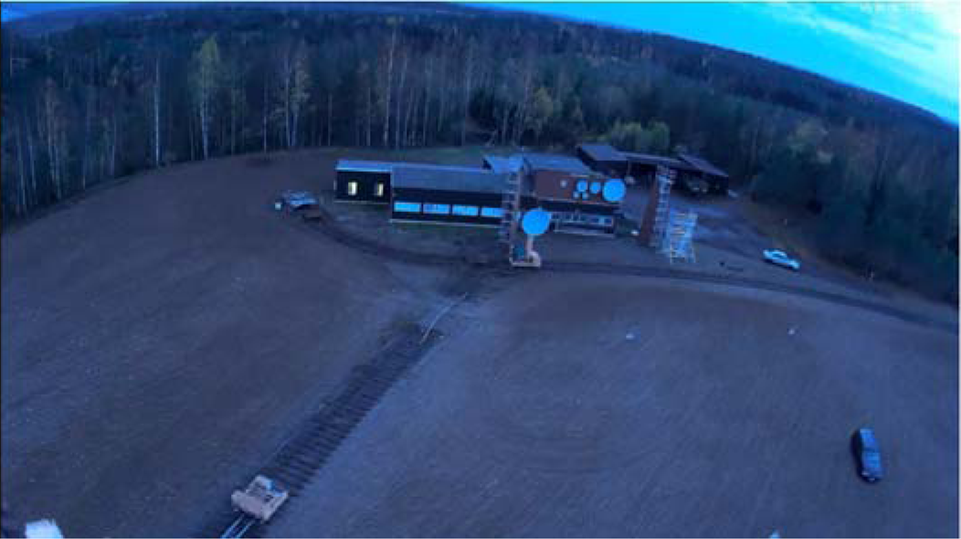
A photograph of the measurement scene taken from the drone is shown in Fig. 3. The scene contains (amongst others) a flat gravel area with a rail track, some corner reflectors of different sizes and a car. In the background, there is a group of buildings and a garage in front of a group of trees.

Fig. 3. Photograph of the measurement scene taken from the drone.
The used radar bandwidth was 5.4–6.0 GHz, the pulse repetition interval (PRI) was 1060 μs, and the ADC sample rate was about 5.1 Gsps. The radar antenna depression angle was 30°. The flight altitude and speed was in the range 25–30 m and 0–5 m/s, respectively. The theoretical best resolutions δ x and δ r in range and cross-range are approximately given by [Reference Chan and Koo23]

Here λ c is the center wavelength (at the center frequency 5.7 GHz), θ a is the 3 dB beamwidth of the antennas (30°), c is the speed of light, and B is the bandwidth (600 MHz).
SAR images generated with attitude (IMU) angles
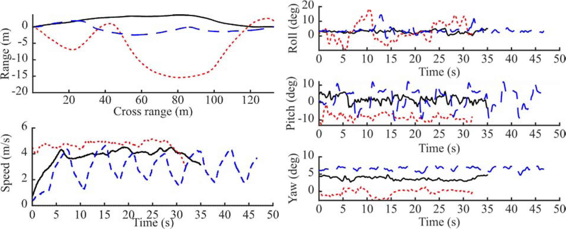
To assess the impact of using attitude angles (roll, pitch, and yaw) recorded by the IMU to adjust for the change in relative positions of the radar and GNSS antenna as the drone moves, three different flight trajectories were used (see Fig. 4). A straight flight trajectory was used as a reference, a zigzag trajectory was used to simulate windy conditions, and a third trajectory with large speed variations was also included. The resulting SAR images can be found in Figs 5–10.

Fig. 4. The flight trajectories (top left) and speed (bottom left) along with roll, pitch, and yaw (right top, mid, and bottom) recorded by the IMU for the straight (solid black), zigzag (dotted red), and varying speed (dashed blue) flights.
Fig. 5. SAR image generated with data from the straight flight trajectory, using RTK position but no IMU data. The image shows pixel intensity relative to the maximum pixel intensity in dB scale, where 0 dB is white and ≤ −70 dB is black. The scene is 150 m × 100 m.
Fig. 6. SAR image generated with data from the straight flight trajectory, using RTK position and IMU data. The image shows pixel intensity relative to the maximum pixel intensity in dB scale, where 0 dB is white and ≤ −70 dB is black. The scene is 150 m × 100 m.
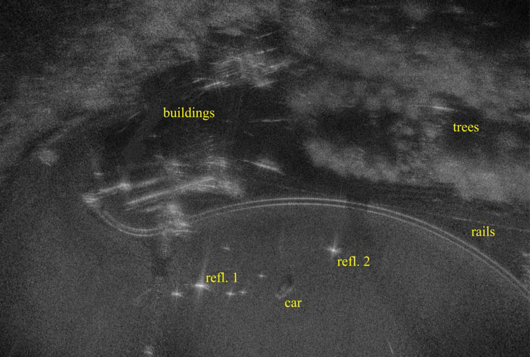
Fig. 7. SAR image generated with data from the zigzag flight trajectory, using RTK position but no IMU data. The image shows pixel intensity relative to the maximum pixel intensity in dB scale, where 0 dB is white and ≤ −70 dB is black. The scene is 150 m × 100 m.

Fig. 8. SAR image generated with data from the zigzag flight trajectory, using RTK position and IMU data. The image shows pixel intensity relative to the maximum pixel intensity in dB scale, where 0 dB is white and ≤ −70 dB is black. The scene is 150 m × 100 m.

Fig. 9. SAR image generated with data from the flight with varying speed, using RTK position but no IMU data. The image shows pixel intensity relative to the maximum pixel intensity in dB scale, where 0 dB is white and ≤ −70 dB is black. The scene is 150 m × 100 m.
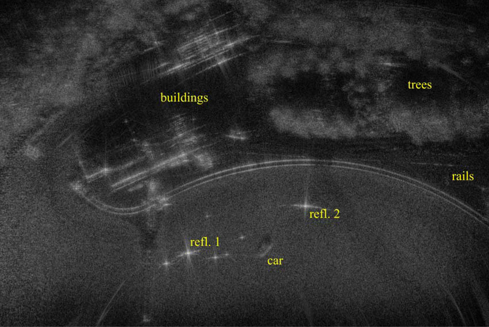
Fig. 10. SAR image generated with data from the flight with varying speed, using RTK position and IMU data. The image shows pixel intensity relative to the maximum pixel intensity in dB scale, where 0 dB is white and ≤ −70 dB is black. The scene is 150 m × 100 m.
Image quality assessment
In this section, the SAR images presented in section ‘SAR images generated with attitude (IMU) angles’ are analyzed using a set of quality measures. The images generated from the measurements along the straight trajectory give the impression of being independent of the compensation of attitude (IMU) angles and looks better to the eye than the images generated with the zigzag trajectory or the flight with varying speed. However, it seems like the quality of the images generated from the latter two flights is improved slightly when attitude angles are used. To investigate and quantify these impressions, a set of quality measures is computed (see Table 1). The image quality measures are presented and discussed in more detail following Table 1.
Table 1. Image quality measures for the SAR images in Figs 5–10, corresponding to the flight trajectories in Fig. 4.

First, the overall sharpness of the image is assessed using a global image sharpness measure from the field of image processing [Reference De and Masilamani28]. It uses the Fourier transform in the range and cross-range directions of an image, and is defined as the percentage of pixels in the transformed image that has an intensity higher than −60 dB relative to the center of the transformed image. Here, a higher percentage indicates a sharper image. We note a slight increase for all the images, albeit very small for the straight path, as attitude data (IMU) is used. The sharpness measure of the image generated with the straight trajectory is considerably higher than those for the zigzag trajectory and the flight with varying speed. Note, however, that the sharpness measures for the three different trajectories are not exactly comparable, since they image slightly different parts of the measurement scene.
Secondly, the side-lobes of the two dominant corner reflectors are analyzed by determining the corresponding 3 dB lobe widths and side-lobe ratios. In each image at least one reflector is seen to have 3 dB lobe widths in the same range as the theoretical resolution. The lobe widths are reduced when using attitude data (IMU) for the zigzag trajectory, while the results for the other two trajectories are ambiguous.
The peak side-lobe ratio is determined as the quotient of the maximum intensity in the main-lobe and side-lobe areas. Here, the main-lobe area is defined as the area inside an ellipse with semi-axes of lengths 3δ x and 3δ r, respectively. Likewise, the side-lobe area is defined as the area inside an ellipse with semi-axes of lengths 10δ x and 10δ r, respectively, but outside the main-lobe ellipse [Reference Vu, Sjögren, Pettersson and Gustavsson29]. When attitude data (IMU) is used, the peak side-lobe ratio is reduced for the zigzag trajectory, and for the flight with varying speed. The peak side-lobe ratios for the straight trajectory, which are lower than the peak side-lobe ratios for the other two trajectories, are slightly increased when attitude data is used.
Some conclusions made from the results in Table 1 are summarized here. Without attitude data (IMU), the straight flight trajectory yields the best image quality in terms of the global image sharpness measure, side-lobe ratios, and 3 dB lobe-widths in cross-range, while the 3 dB lobe-widths in range is not lower for all combinations. However, when attitude data is used, the 3 dB lobe width in cross-range of Reflector 2 is higher for the straight trajectory than the other two trajectories. Using attitude data improves all quality measures for the zigzag trajectory. For the trajectory with varying speed, all quality measures except the 3 dB lobe width in cross-range of Reflector 1 are improved or approximately equal when attitude data is used. For the straight trajectory, however, the side-lobe levels for both reflectors as well as the 3 dB lobe widths in range and cross-range of Reflector 1 are higher, although still low, when attitude data is used. Possible explanations for the slightly lower quality with attitude data could be the limited accuracy of the IMU sensor and in the measured locations of the antenna phase centers.
The zigzag trajectory exhibits the largest variation in roll angle, while the flight with varying speed exhibits the largest variation in pitch angle, as seen in Fig. 4. Intuitively, variations in roll angle can be expected to affect the image quality more than variations in pitch angle, since a varying roll angle mostly changes the relative antenna positions in the range direction, while variations in the pitch angle mostly changes the relative antenna altitude. Although the overall image sharpness measure and quality measures for Reflector 1 support this expectation, the quality measures for Reflector 2 point in the opposite direction.
To further analyze the main and side-lobes, the point spread function (PSF) of a target located at the position of Reflector 1 and Reflector 2 is computed for the three trajectories. More specifically, the return of an ideal, isotropically scattering point target is used in the BP algorithm to create an image, assuming the measured positions are the exact position of the antenna phase centers. Here, the radar antennas are assumed to have uniform gain within a 30o lobe, and no gain outside that lobe. The result is compared to the images generated with measured data, using position data as well as attitude data (see Figs 11 and 12). The measured and simulated results agree well in the range direction, while the side-lobes in the cross-range direction are much higher for the measured image, especially for the non-straight trajectories. Note, however, that the corner reflector is not an ideal point target, and that a perfect match between measurements and simulations is not realistic. It is also interesting to note the smoother range pattern for the PSF computed with the trajectory with varying speed, compared to the other trajectories. A further analysis of varying resolution due to non-ideal trajectories can be found in [Reference Catapano, Gennarelli, Ludeno, Noviello, Esposito, Renga, Fasano and Soldovieri11].
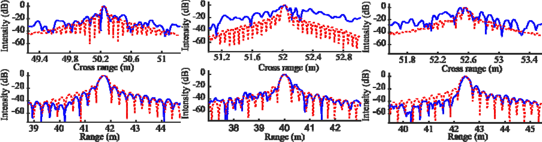
Fig. 11. Simulated PSF of a point target located at the position of Reflector 1 (dotted red) compared to measured image intensity (solid blue) for (a) the straight trajectory, (b) the zigzag trajectory, and (c) the trajectory with varying speed. Position and attitude data were used, and the antenna positions are assumed to be exact for the simulated PSF.
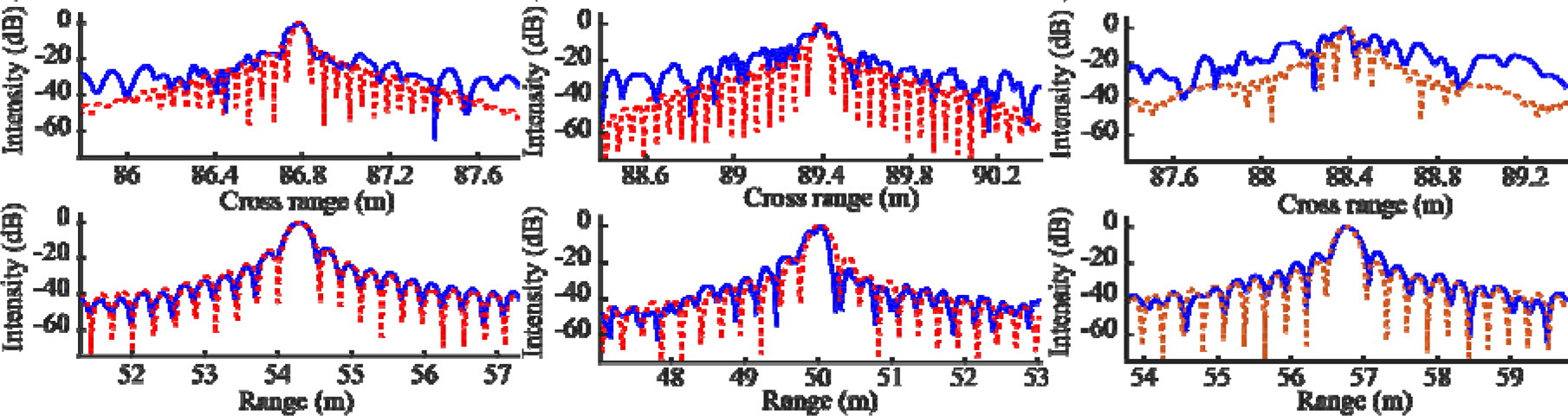
Fig. 12. Simulated PSF of a point target located at the position of Reflector 2 (dotted red) compared to measured image intensity (solid blue) for (a) the straight trajectory, (b) the zigzag trajectory, and (c) the trajectory with varying speed. Position and attitude data were used, and the antenna positions are assumed to be exact for the simulated PSF.
SAR images generated onboard in near real time
The measurement system presented in this paper is capable of generating SAR images using a BP algorithm implemented on the GPU of the onboard computer, as described in section ‘Image formation onboard close to real time’. The SAR sub-images are transmitted to a PC on the ground using the Wi-Fi data link.
SAR images generated onboard the UAV can be found in Fig. 13. Here, a relatively straight flight trajectory was chosen, since attitude data presently cannot be accessed by the onboard computer. The scene is 120 m × 100 m, and the pixel size is the theoretical resolution given in equation (1).
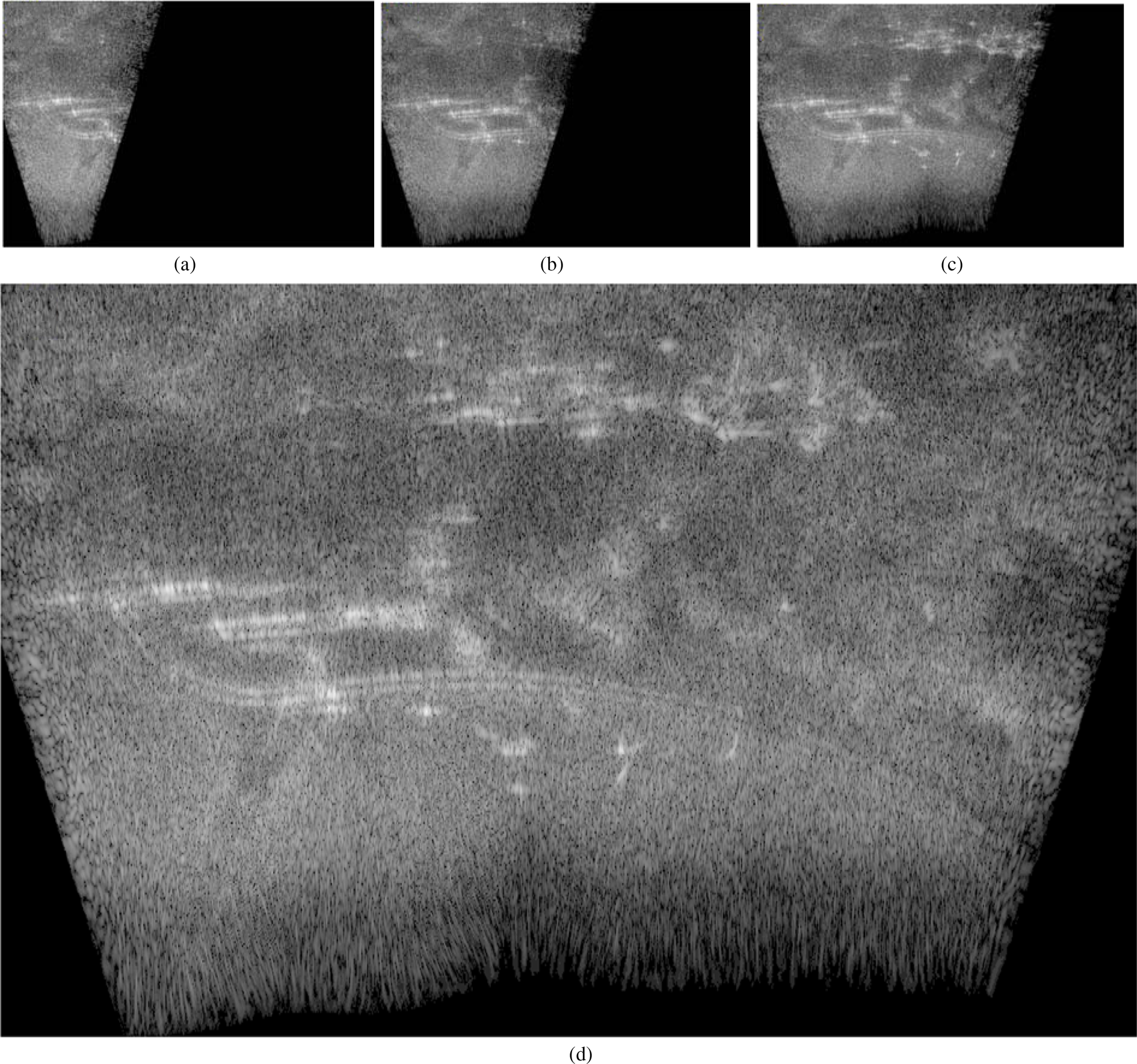
Fig. 13. SAR images generated in near real time onboard the drone, and transmitted to a PC on the ground using a Wi-Fi data link. The figure shows four of the images, (a)–(d), transmitted during the flight. The images show pixel intensity relative to the maximum pixel intensity in dB scale, where 0 dB is white and ≤−70 dB is black. The scene is 120 m × 100 m.
The Shannon–Nyquist sampling criterion needs to be fulfilled, that is, at least two samples per wavelength are needed [Reference Showman, Richards, Scheer and Holm1]. With a maximum frequency of 6 GHz and 3 dB antenna lobe-width of θ a =30°, it means that the distance travelled between two samples needs to fulfil

Here, we choose to consider every 20th radar sweep, that is, the decimation factor is 20. When the speed of the UAV is ~2 m/s and the PRI is 1060 μs, this is sufficient to fulfil the sampling criterion, as the distance travelled between every 20th sweep is Δdist ≈ 2 m/s × 20 × 1060 × 10−6 s ≈ 0.042 m. Ideally, however, over-sampling with at least a factor of ~2 is desirable [Reference Showman, Richards, Scheer and Holm1]. The relatively low quality of the SAR image generated onboard (Fig. 13) compared to the SAR images generated post flight (Figs 5–10) are likely caused by the coarse sampling in cross-range and the coarse grid of the SAR image generated onboard.
SAR measurements are naturally not working in true real time since the technique is based on multiple measurements along a flight path. Mainly two factors limit the real-time performance; the radar data collection and the onboard SAR processing. The onboard computer processes blocks of 100 radar sweeps at a time, with which a PRI of 1060 μs and a decimation factor of 20 correspond to slightly more than 2 s. With the scene size and resolution chosen here, processing a block of 100 sweeps takes ~2 s, which means that the SAR processing is not the limiting factor. The processing time can likely be improved by increasing the hardware processing capacity or by using more optimized software.
In the example considered here, the onboard SAR processing can just about keep up. Increasing the scene size or resolution will slow down the SAR processing, resulting in the image generation falling behind more and more. Likewise, increasing the speed of the UAV, which requires a reduced decimation factor, will also slow down the SAR processing. On the other hand, decreasing the scene size, resolution, or speed of the UAV speeds up the processing.
Conclusion
We presented a SAR system assembled on a small UAV, based on low-cost open-source and off-the-shelf components: a 5–6 GHz radar, a GNSS/RTK position sensor, an autopilot including IMU sensor, and a single-board computer with GPU. SAR images were generated, showing 3 dB lobe-widths close to the theoretically predicted resolution.
We found that flying in a zigzag trajectory, or varying the speed, resulted in larger 3 dB lobe-widths, and also larger peak side-lobe ratios, compared to a relatively straight trajectory with more constant speed. This is likely due to the changes in the relative positions of the GNSS and radar antennas as the drone tilts back and forth. The 3 dB lobe-widths and peak side-lobe ratios for these cases were, for the most part, improved when we made use of the attitude data (roll, pitch, and yaw) recorded by the IMU. The 3 dB lobe-widths were in some cases close to those of the straight trajectory, and in the same order as the theoretical resolution. The side-lobe ratios, however, were higher than those for the straight trajectory, even when attitude data were used.
The overall sharpness of the images was also analyzed using a global image sharpness measure from the field of image processing, which lead to much the same conclusion as above: the quality of the SAR images was reduced when the flight trajectory was curved or the speed was varied, something that could be somewhat remedied using recorded attitude data.
Possible ways to improve the results further, and approach the quality achieved with the straight trajectory, could be to use a more accurate IMU sensor, or to compute and make use of the frequency-dependent antenna phase centers. Further experiments with many varying flight trajectories and measurement scenes are also highly relevant future work. Using autofocus algorithms can likely also improve the image quality but leads to an increased computational burden.
Finally, SAR images generated in near real time onboard the UAV, and transmitted to a PC using a Wi-Fi data link, were presented. The SAR processing speed was enough to keep up with the data collection for the example considered, where the speed of the UAV was ~2 m/s and the scene size was 120 m × 100 m with range and cross-range resolution 0.25 and 0.05 m, respectively. Increasing the demands would require more efficient software or hardware.
The SAR system we presented was built using low-cost off-the-shelf or open-source hardware. Furthermore, the type of equipment used is rapidly becoming better and less expensive, a development we believe will make similar systems attractive for a wide variety of applications.
Acknowledgements
This work has been funded by the Swedish Armed Forces R&D programme for Sensors and low observables (FoT SoS, AT.9220420).
 Jan Svedin received the M.Sc. degree in applied physics and electrical engineering and Ph.D. degree in theoretical physics from the Linköping Institute of Technology, Linköping, Sweden, in 1986 and 1991, respectively. He is presently a Deputy Director of Research within the Radar Systems Department at FOI, the Swedish Defence Research Agency. His research interests include millimeter wave technology and its various applications, including antennas, components, and manufacturing technologies for sensor imaging systems.
 Anders Bernland received the M.Sc. degree in engineering mathematics and the Ph.D. degree in electromagnetic theory from Lund University, Lund, Sweden, in 2007 and 2012, respectively. He is presently a researcher within radar systems at FOI, Swedish Defence Research Agency. His research interests include electromagnetic wave propagation and scattering, antennas, computational electromagnetics, and computational design optimization.
 Andreas Gustafsson received his M.Sc. in engineering physics at Umeå University, Sweden, in 1996. Since 1997 he has been employed at FOI, Swedish Defence Research Agency, working with RF front-end technology. In 2004, he received (as first author) the Radar Prize at the European Microwave Week for the design and evaluation of an experimental compact 16-channel smart-skin digital beam forming X-band antenna module. During the last 15 years, he has also been working with multistatic arrays with several publications in that field. He is also active within the research areas of radar systems, microwave subsystem design, and MMIC-design. He is the author or co-author of more than 30 scientific publications.
 Eric Claar is currently pursuing the M.Sc. degree in Electronics Design at Linköping University, Sweden. He is working on his master thesis at FOI, Swedish Defence Research Agency, which focuses on near real-time SAR processing.
 John Luong is currently a student at Linköping University, Sweden, working towards receiving the M.Sc. degree in Electronics Design. He is doing his master thesis at FOI, Swedish Defence Research Agency, about near real-time SAR processing.


 Open access