


1 Introduction
One of the major challenges facing the wind energy sector is the growing need to accurately model large-scale wind turbines, numerically or experimentally. The difficulty of this task is realized when considering the requirement of full dynamic similarity for the given physical problem. In general, the concept of dynamic similarity stipulates that the relevant non-dimensional parameters be matched between a model or simulation and the full-scale application, as well as the non-dimensional boundary conditions, to fully capture the associated dynamics. For the aerodynamics of wind turbines, the governing parameters for the canonical case are the Reynolds number ( $Re$
), tip speed ratio (
$Re$
), tip speed ratio ( $\unicode[STIX]{x1D706}$
) and Mach number (
$\unicode[STIX]{x1D706}$
) and Mach number ( $Ma$
):
$Ma$
):
 $$\begin{eqnarray}Re=\frac{\unicode[STIX]{x1D70C}U^{\ast }L^{\ast }}{\unicode[STIX]{x1D707}},\quad \unicode[STIX]{x1D706}=\frac{\unicode[STIX]{x1D714}R}{U^{\ast }},\quad Ma=\frac{\unicode[STIX]{x1D714}R}{a}.\end{eqnarray}$$
Here $\unicode[STIX]{x1D70C}$
and
$\unicode[STIX]{x1D70C}$
and $\unicode[STIX]{x1D707}$
are the fluid density and dynamic viscosity, respectively;
$\unicode[STIX]{x1D707}$
are the fluid density and dynamic viscosity, respectively; $U^{\ast }$
is a characteristic velocity scale of the flow;
$U^{\ast }$
is a characteristic velocity scale of the flow; $L^{\ast }$
is a characteristic length scale (such as the radius of the turbine,
$L^{\ast }$
is a characteristic length scale (such as the radius of the turbine, $R$
, or its chord length,
$R$
, or its chord length, $c$
);
$c$
); $\unicode[STIX]{x1D714}$
is the angular velocity of the turbine rotor; and
$\unicode[STIX]{x1D714}$
is the angular velocity of the turbine rotor; and $a$
is the local speed of sound. To satisfy the non-dimensional boundary conditions, geometric similarity with the full scale is required. Deviation from this will result in additional length-scale ratios, and hence additional non-dimensional parameters that are not found at the full scale.
$a$
is the local speed of sound. To satisfy the non-dimensional boundary conditions, geometric similarity with the full scale is required. Deviation from this will result in additional length-scale ratios, and hence additional non-dimensional parameters that are not found at the full scale.
Owing to the inverse relationship with velocity in $Re$
and
$Re$
and $\unicode[STIX]{x1D706}$
, it is challenging to simultaneously match these non-dimensional parameters in model scale testing. Consequently, many wind turbine experiments (both horizontal- and vertical-axis wind turbines, or HAWTs and VAWTs for short) are performed at reduced Reynolds numbers and/or tip speed ratios (Vermeer, Sørensen & Crespo Reference Vermeer, Sørensen and Crespo2003). There has been some justification for this methodology for HAWT studies (Chamorro, Arndt & Sotiropoulos Reference Chamorro, Arndt and Sotiropoulos2011), where a value of
$\unicode[STIX]{x1D706}$
, it is challenging to simultaneously match these non-dimensional parameters in model scale testing. Consequently, many wind turbine experiments (both horizontal- and vertical-axis wind turbines, or HAWTs and VAWTs for short) are performed at reduced Reynolds numbers and/or tip speed ratios (Vermeer, Sørensen & Crespo Reference Vermeer, Sørensen and Crespo2003). There has been some justification for this methodology for HAWT studies (Chamorro, Arndt & Sotiropoulos Reference Chamorro, Arndt and Sotiropoulos2011), where a value of $Re_{D}$
(based on hub-height wind velocity and rotor diameter) of at least 93 000 is specified for the flow dynamics to be independent of the Reynolds number. Measurements in the far wake of a small model turbine showed less of a dependence on
$Re_{D}$
(based on hub-height wind velocity and rotor diameter) of at least 93 000 is specified for the flow dynamics to be independent of the Reynolds number. Measurements in the far wake of a small model turbine showed less of a dependence on $Re$
for the first and second velocity moments. However, the Reynolds numbers tested in that study were at least an order of magnitude lower than what can be considered a full-scale value (
$Re$
for the first and second velocity moments. However, the Reynolds numbers tested in that study were at least an order of magnitude lower than what can be considered a full-scale value ( $1.66\times 10^{4}<Re_{D}<1.73\times 10^{5}$
), and it is likely that flow regimes are different. Another often-cited study is the review article of Vries (Reference Vries1983), wherein the problem of scaling is addressed and a value of the Reynolds number (based on the chord length and relative velocity),
$1.66\times 10^{4}<Re_{D}<1.73\times 10^{5}$
), and it is likely that flow regimes are different. Another often-cited study is the review article of Vries (Reference Vries1983), wherein the problem of scaling is addressed and a value of the Reynolds number (based on the chord length and relative velocity), $Re_{c}>3\times 10^{5}$
, is given as a possible minimum. However, this value was suggested without a convincing justification. Interestingly, the review article notes that a compressed-air wind tunnel is the only way to realize the matching of all non-dimensional parameters, suggesting that the author was well aware of the scaling issues associated with model wind turbine tests.
$Re_{c}>3\times 10^{5}$
, is given as a possible minimum. However, this value was suggested without a convincing justification. Interestingly, the review article notes that a compressed-air wind tunnel is the only way to realize the matching of all non-dimensional parameters, suggesting that the author was well aware of the scaling issues associated with model wind turbine tests.
In the closely related field of steady two-dimensional airfoil aerodynamics, similar trends have been observed. The minimum $Re_{c}$
that is required to achieve Reynolds-number invariance in the lift and drag coefficients (
$Re_{c}$
that is required to achieve Reynolds-number invariance in the lift and drag coefficients ( $C_{l}$
and
$C_{l}$
and $C_{d}$
, respectively) is still a subject of ongoing debate. Based on Miley (Reference Miley1982), values of
$C_{d}$
, respectively) is still a subject of ongoing debate. Based on Miley (Reference Miley1982), values of $Re_{c}\leqslant 500\,000$
are often cited as low, where significant portions of the boundary layer can be expected to be laminar, which alters the separation and stall characteristics of the airfoil. On the other hand, a sufficiently high Reynolds number is considered to be
$Re_{c}\leqslant 500\,000$
are often cited as low, where significant portions of the boundary layer can be expected to be laminar, which alters the separation and stall characteristics of the airfoil. On the other hand, a sufficiently high Reynolds number is considered to be $Re_{c}>3\times 10^{6}$
, where effects such as stall and laminar separation are reduced due to the boundary layer being turbulent over most of the airfoil. These suggested bounds may in fact be conservative, but it is generally agreed that below an
$Re_{c}>3\times 10^{6}$
, where effects such as stall and laminar separation are reduced due to the boundary layer being turbulent over most of the airfoil. These suggested bounds may in fact be conservative, but it is generally agreed that below an $Re_{c}$
of approximately 500 000 additional aerodynamic phenomena arise which complicate the measurement of a global flow variable such as lift coefficient (Mueller Reference Mueller1985).
$Re_{c}$
of approximately 500 000 additional aerodynamic phenomena arise which complicate the measurement of a global flow variable such as lift coefficient (Mueller Reference Mueller1985).
Although physically smaller in scale compared to modern HAWT designs, field-scale VAWTs still achieve Reynolds numbers that are higher than those easily matched in laboratory studies. For instance, the FloWind VAWT (FloWind 1996), with a rotor diameter of $D=19.2~\text{m}$
, achieved a Reynolds number of
$D=19.2~\text{m}$
, achieved a Reynolds number of $Re_{D}=\unicode[STIX]{x1D70C}UD/\unicode[STIX]{x1D707}\approx 15\times 10^{6}$
at an operational tip speed ratio of
$Re_{D}=\unicode[STIX]{x1D70C}UD/\unicode[STIX]{x1D707}\approx 15\times 10^{6}$
at an operational tip speed ratio of $\unicode[STIX]{x1D706}\approx 4.3$
and standard atmospheric conditions. To capture the effects of Reynolds-number changes at the blade level, a chord-based Reynolds number can be defined for convenience, which uses the maximum relative speed possible at the rotor blade,
$\unicode[STIX]{x1D706}\approx 4.3$
and standard atmospheric conditions. To capture the effects of Reynolds-number changes at the blade level, a chord-based Reynolds number can be defined for convenience, which uses the maximum relative speed possible at the rotor blade, $U+\unicode[STIX]{x1D714}R$
, as the velocity scale. For the FloWind unit at the conditions given previously, this translates to a blade Reynolds number of
$U+\unicode[STIX]{x1D714}R$
, as the velocity scale. For the FloWind unit at the conditions given previously, this translates to a blade Reynolds number of $Re_{c}=\unicode[STIX]{x1D70C}c(U+\unicode[STIX]{x1D714}R)/\unicode[STIX]{x1D707}\approx 3.0\times 10^{6}$
. Smaller wind turbines, such as those that have been used at the Stanford University Field Laboratory for Optimized Wind Energy (FLOWE), still achieved relatively high
$Re_{c}=\unicode[STIX]{x1D70C}c(U+\unicode[STIX]{x1D714}R)/\unicode[STIX]{x1D707}\approx 3.0\times 10^{6}$
. Smaller wind turbines, such as those that have been used at the Stanford University Field Laboratory for Optimized Wind Energy (FLOWE), still achieved relatively high $Re_{D}\approx 760\,000$
and
$Re_{D}\approx 760\,000$
and $Re_{c}\approx 420\,000$
(at operational point
$Re_{c}\approx 420\,000$
(at operational point $\unicode[STIX]{x1D706}\approx 2.3$
(Dabiri Reference Dabiri2011)). This indicates that, despite the method of operation, be it vertical or horizontal rotation, most commercial field-scale wind turbines operate outside the Reynolds-number range achievable in traditional laboratories.
$\unicode[STIX]{x1D706}\approx 2.3$
(Dabiri Reference Dabiri2011)). This indicates that, despite the method of operation, be it vertical or horizontal rotation, most commercial field-scale wind turbines operate outside the Reynolds-number range achievable in traditional laboratories.
In this study, we aim to address the question of scaling independence with Reynolds number as it applies to VAWTs. A five-bladed model turbine, based on an existing commercial design, was fabricated for this study. The model accurately replicates the full-scale geometry with a $1/22.5$
scale ratio. Using a specialized wind tunnel that utilizes compressed air as the working fluid, the full-scale Reynolds numbers and tip speed ratios were matched and even exceeded using the relatively small-scale model, while the Mach number was kept low (similar to the field values) to avoid any flow compressibility effects. The model turbine rotation in these experiments was solely powered by aerodynamic forces (self-spinning), including the start-up phase (from
$1/22.5$
scale ratio. Using a specialized wind tunnel that utilizes compressed air as the working fluid, the full-scale Reynolds numbers and tip speed ratios were matched and even exceeded using the relatively small-scale model, while the Mach number was kept low (similar to the field values) to avoid any flow compressibility effects. The model turbine rotation in these experiments was solely powered by aerodynamic forces (self-spinning), including the start-up phase (from $\unicode[STIX]{x1D706}=0$
to operational values), without any external inputs. This is in contrast to several low-Reynolds-number model studies where the turbine rotor is artificially spun up (typically with an external motor) to the desired tip speed ratio. This allows for the interpretation of the experimental results in the context of field-scale turbine behaviour without any assumptions or corrections.
$\unicode[STIX]{x1D706}=0$
to operational values), without any external inputs. This is in contrast to several low-Reynolds-number model studies where the turbine rotor is artificially spun up (typically with an external motor) to the desired tip speed ratio. This allows for the interpretation of the experimental results in the context of field-scale turbine behaviour without any assumptions or corrections.
2 Experimental facility and model
While the concept of using a compressed gas as a working fluid for increased Reynolds numbers is not new (see e.g. Jacobs & Abbott Reference Jacobs and Abbott1933; Zagarola & Smits Reference Zagarola and Smits1998; Llorente et al.
Reference Llorente, Gorostidi, Jacobs, Timmer, Munduate and Pires2014), the implementation of this method for testing rotating wind turbine models at full-scale $Re$
has not been previously attempted. To achieve this, a specialized wind tunnel at Princeton University known as the High Reynolds number Test Facility (HRTF) was used. The HRTF is a recirculating type, low-velocity, high-static-pressure tunnel that uses compressed air as the working fluid. The facility can support static pressures,
$Re$
has not been previously attempted. To achieve this, a specialized wind tunnel at Princeton University known as the High Reynolds number Test Facility (HRTF) was used. The HRTF is a recirculating type, low-velocity, high-static-pressure tunnel that uses compressed air as the working fluid. The facility can support static pressures, $p_{s}$
, of up to 24 MPa (3500 psia, or in excess of 233 bar) and free-stream velocities,
$p_{s}$
, of up to 24 MPa (3500 psia, or in excess of 233 bar) and free-stream velocities, $U$
, in the test section of up to
$U$
, in the test section of up to $10~\text{m}~\text{s}^{-1}$
. It is the ability to achieve high Reynolds numbers at relatively low velocities that permits studies of rotating flows, since it enables tests at realistic rotational rates. The relationship between tunnel pressure and density is given by
$10~\text{m}~\text{s}^{-1}$
. It is the ability to achieve high Reynolds numbers at relatively low velocities that permits studies of rotating flows, since it enables tests at realistic rotational rates. The relationship between tunnel pressure and density is given by $\unicode[STIX]{x1D70C}=p_{s}/(ZRT)$
, where
$\unicode[STIX]{x1D70C}=p_{s}/(ZRT)$
, where $R$
is the specific gas constant for air,
$R$
is the specific gas constant for air, $T$
the tunnel temperature and
$T$
the tunnel temperature and $Z$
the compressibility factor. For dry air
$Z$
the compressibility factor. For dry air $Z$
changes by only 10 % for static pressures in the range 1–233 bar, meaning that density changes nearly linearly with static pressure in the test section. The key to this facility is twofold: firstly, the dynamic viscosity of air has a weak dependence on pressure, changing by only 30 % over the same pressure range given above; and secondly, the Mach number remains well below the compressible limit for all tests, since the speed of sound is also a very weak function of pressure. For all data, the exact density and viscosity of the compressed air are calculated using the real-gas relationship with measurements of
$Z$
changes by only 10 % for static pressures in the range 1–233 bar, meaning that density changes nearly linearly with static pressure in the test section. The key to this facility is twofold: firstly, the dynamic viscosity of air has a weak dependence on pressure, changing by only 30 % over the same pressure range given above; and secondly, the Mach number remains well below the compressible limit for all tests, since the speed of sound is also a very weak function of pressure. For all data, the exact density and viscosity of the compressed air are calculated using the real-gas relationship with measurements of $p_{s}$
and
$p_{s}$
and $T$
from the test section (this method is outlined in Zagarola (Reference Zagarola1996)), but for convenience plots are shown with the static tunnel pressure as a reference point.
$T$
from the test section (this method is outlined in Zagarola (Reference Zagarola1996)), but for convenience plots are shown with the static tunnel pressure as a reference point.
A schematic of the HRTF is shown in figure 1. It contains two working sections with a total length of 4.88 m. Each test section length has a circular cross-section with an inside diameter of 0.49 m. Preceding the test section is a contraction with an area ratio of 2.2 : 1 in which a series of honeycomb straighteners and flow conditioning screens are located. These measures produce a laminar slug flow in the test section with a turbulence level of 0.3 % at the lowest Reynolds number and 1.1 % at the highest values of $Re$
(Jiménez, Hultmark & Smits Reference Jiménez, Hultmark and Smits2010). Free-stream velocity is measured via a pitot-static tube located upstream of the turbine model and connected to a Validyne DP-15 differential pressure transducer with a range of 13.79 kPa. The HRTF was previously used in high-Reynolds-number studies of the wake of a suboff model (Jiménez et al.
Reference Jiménez, Hultmark and Smits2010; Ashok, Van Buren & Smits Reference Ashok, Van Buren and Smits2015) and zero-pressure-gradient turbulent boundary layers (Vallikivi, Hultmark & Smits Reference Vallikivi, Hultmark and Smits2015); further details on the facility itself can be found in those papers.
$Re$
(Jiménez, Hultmark & Smits Reference Jiménez, Hultmark and Smits2010). Free-stream velocity is measured via a pitot-static tube located upstream of the turbine model and connected to a Validyne DP-15 differential pressure transducer with a range of 13.79 kPa. The HRTF was previously used in high-Reynolds-number studies of the wake of a suboff model (Jiménez et al.
Reference Jiménez, Hultmark and Smits2010; Ashok, Van Buren & Smits Reference Ashok, Van Buren and Smits2015) and zero-pressure-gradient turbulent boundary layers (Vallikivi, Hultmark & Smits Reference Vallikivi, Hultmark and Smits2015); further details on the facility itself can be found in those papers.

Figure 1. The High Reynolds number Test Facility (HRTF) located at the Princeton Gas Dynamics Laboratory. The external motor (a) drives an internal impeller pump, which moves compressed air though the return section and on to the flow conditioning and contraction at (b), where it next enters the two working sections at (c). The facility is designed to produce laminar slug flow inside the test section at low turbulence levels.
2.1 Wind turbine model
One of the primary challenges associated with testing in a pressurized environment is the large mechanical loads imposed on the model, which scale proportionally with the density. This can be shown by considering the power and thrust coefficients, which are the non-dimensionalized shaft power and axial thrust,
 $$\begin{eqnarray}C_{p}=\frac{\unicode[STIX]{x1D70F}\unicode[STIX]{x1D714}}{{\textstyle \frac{1}{2}}\unicode[STIX]{x1D70C}U^{3}A},\quad C_{t}=\frac{F_{t}}{{\textstyle \frac{1}{2}}\unicode[STIX]{x1D70C}U^{2}A},\end{eqnarray}$$
where $A=S\times D$
is the rotor swept area (
$A=S\times D$
is the rotor swept area ( $S$
is the rotor span and
$S$
is the rotor span and $D$
its diameter),
$D$
its diameter), $\unicode[STIX]{x1D70F}$
is the total aerodynamic torque on the central shaft and
$\unicode[STIX]{x1D70F}$
is the total aerodynamic torque on the central shaft and $F_{t}$
is the axial thrust force. It is important to note that
$F_{t}$
is the axial thrust force. It is important to note that $C_{p}$
and
$C_{p}$
and $C_{t}$
, or any other dependent, non-dimensional group for this physical problem, rely only upon the parameters set in (1.1). This means that different combinations of
$C_{t}$
, or any other dependent, non-dimensional group for this physical problem, rely only upon the parameters set in (1.1). This means that different combinations of $U$
,
$U$
, $\unicode[STIX]{x1D70C}$
and
$\unicode[STIX]{x1D70C}$
and $\unicode[STIX]{x1D714}$
can be used to vary the physical loads, but produce the same
$\unicode[STIX]{x1D714}$
can be used to vary the physical loads, but produce the same $Re$
and
$Re$
and $\unicode[STIX]{x1D706}$
, and thus the same values of
$\unicode[STIX]{x1D706}$
, and thus the same values of $C_{p}$
and
$C_{p}$
and $C_{t}$
(as long as
$C_{t}$
(as long as $Ma$
is kept low enough to avoid compressibility effects, which is the case with the present experiments). This also implies that, due to the variable tunnel density, a model will see up to 230 times the mechanical loads (
$Ma$
is kept low enough to avoid compressibility effects, which is the case with the present experiments). This also implies that, due to the variable tunnel density, a model will see up to 230 times the mechanical loads ( $\unicode[STIX]{x1D70F}$
and
$\unicode[STIX]{x1D70F}$
and $F_{t}$
) in the HRTF as a model in an atmospheric tunnel at the same velocity and physical scale.
$F_{t}$
) in the HRTF as a model in an atmospheric tunnel at the same velocity and physical scale.
For these experiments a five-bladed model rotor geometry was used that is based on a commercial unit produced by Wing Power Energy (WPE: this unit was previously used at the FLOWE test site, see § 2.4). The airfoil blades were accurately reproduced by a five-axis computer numerical control (CNC) milling machine starting from solid blocks of 7075 aluminium alloy. Small geometric changes to the model hub and support tower were made to accommodate the increased loads. The full-scale airfoil has a small surface section removed on the trailing edge of the pressure side to aid in self-starting. This detail was not replicated on the model, as it is not expected to significantly affect the turbine performance in steady operational conditions, and the model had no self-starting issues. The final model airfoil retains the same overall profile as the full scale, which closely resembles a NACA 0021 airfoil. The area-averaged root-mean-square (r.m.s.) roughness height of the model airfoil was measured with a three-dimensional confocal laser microscope (Olympus LEXT OLS4000) and was found to be
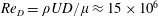
 $S_{q}=0.5\pm 0.25~\unicode[STIX]{x03BC}\text{m}$
. Details of the final model geometry are given in table 1. In addition, a full three-dimensional computer model is available upon request. Preliminary bench testing indicated the model should be kept under a rotational speed of 1500 r.p.m. during operation to minimize any mechanical vibrations in the model fixture. This is reflected in the maximum achievable
$S_{q}=0.5\pm 0.25~\unicode[STIX]{x03BC}\text{m}$
. Details of the final model geometry are given in table 1. In addition, a full three-dimensional computer model is available upon request. Preliminary bench testing indicated the model should be kept under a rotational speed of 1500 r.p.m. during operation to minimize any mechanical vibrations in the model fixture. This is reflected in the maximum achievable $\unicode[STIX]{x1D706}$
for given experimental conditions.
$\unicode[STIX]{x1D706}$
for given experimental conditions.
Table 1. Model geometry.

2.2 Instrumentation

Figure 2. Rendering of VAWT model inside cut-away of HRTF test section. Labels correspond to (a) five-bladed VAWT model, (b) tower housing, (c) six-component force/moment sensor, (d) torque transducer with speed encoder, and (e) magnetic hysteresis brake for speed control. Red arrow gives direction of flow. Detail view of VAWT model is shown with dimensions at right.
Accurate resolution of the forces and torques produced by the model turbine was accomplished with a measurement and control stack located inside the pressurized environment of the HRTF. The measurement stack interfaces with the turbine tower and provides control of the model rotational speed. The entire measurement stack and turbine set-up is shown in the schematic of figure 2. The turbine hub is located in the tunnel centreline and is bolted to the main drive shaft. The entire rotating assembly is supported by the central tower, which itself is mounted onto a three-axis force/moment (six-component) transducer (JR3 Inc., model 75E20A4). The central shaft is located inside the tower by two bearings. It transfers power through a central hole in the force sensor and is connected on the opposite side to a torque transducer/speed encoder (Magtrol, model TM-305, with a dynamic torque range of $\pm 2~\text{N}~\text{m}$
) via a flexible coupling. The rotor speed is controlled by a magnetic hysteresis brake (Magtrol, model AHB-3), located directly after the torque transducer and connected to the shaft via another flexible coupling. In this way, the applied brake torque on the rotor is directly measured, without any losses. Note that the torsional load applied by the brake in this experiment is directly equivalent to a generator load on a field turbine. Individual operating points for the model are set using a fixed brake load and a constant tunnel velocity. At each point, data are sampled at 20 kHz via a National Instruments PCI-6123 card for a period of 300 rotations, from which the relevant statistics are calculated. An overview of the system uncertainties associated with the processed data is shown in table 2.
$\pm 2~\text{N}~\text{m}$
) via a flexible coupling. The rotor speed is controlled by a magnetic hysteresis brake (Magtrol, model AHB-3), located directly after the torque transducer and connected to the shaft via another flexible coupling. In this way, the applied brake torque on the rotor is directly measured, without any losses. Note that the torsional load applied by the brake in this experiment is directly equivalent to a generator load on a field turbine. Individual operating points for the model are set using a fixed brake load and a constant tunnel velocity. At each point, data are sampled at 20 kHz via a National Instruments PCI-6123 card for a period of 300 rotations, from which the relevant statistics are calculated. An overview of the system uncertainties associated with the processed data is shown in table 2.
Table 2. Error sources. Listed uncertainties include linearity, hysteresis and temperature influences combined in an r.m.s. sense for each sensor.

2.3 Experiment test procedure
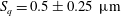
Tests were performed at various Reynolds numbers in the range $5\times 10^{5}<Re_{D}<5\times 10^{6}$
, obtained using different combinations of static pressure and velocity. For a given test condition,
$5\times 10^{5}<Re_{D}<5\times 10^{6}$
, obtained using different combinations of static pressure and velocity. For a given test condition, $p_{s}$
and
$p_{s}$
and $U$
are held constant while the unloaded (zero brake load) model is allowed to self-start completely unassisted and reach the maximum rotational speed (free-spin condition). Once a steady operating point is reached, various braking loads are applied to the model to control the rotational speed (thereby the tip speed ratio), and the corresponding values of
$U$
are held constant while the unloaded (zero brake load) model is allowed to self-start completely unassisted and reach the maximum rotational speed (free-spin condition). Once a steady operating point is reached, various braking loads are applied to the model to control the rotational speed (thereby the tip speed ratio), and the corresponding values of $\unicode[STIX]{x1D70F}$
and
$\unicode[STIX]{x1D70F}$
and $\unicode[STIX]{x1D714}$
measured. In this way,
$\unicode[STIX]{x1D714}$
measured. In this way, $Re_{D}$
stays constant for an entire test while
$Re_{D}$
stays constant for an entire test while $\unicode[STIX]{x1D714}$
(and hence
$\unicode[STIX]{x1D714}$
(and hence $\unicode[STIX]{x1D706}$
and
$\unicode[STIX]{x1D706}$
and $Re_{c}$
) is varied.
$Re_{c}$
) is varied.
2.4 FLOWE field data
In addition to the small-scale experiments, data have been gathered for a single turbine at the Field Laboratory for Optimized Wind Energy (FLOWE) located in the Antelope Valley in northern Los Angeles County, California, USA. This site has been used previously for field measurements on other full-scale VAWT units (Dabiri Reference Dabiri2011; Kinzel, Mulligan & Dabiri Reference Kinzel, Mulligan and Dabiri2012). The terrain at the site is characterized by flat desert for at least 1.5 km in each direction from the array. The turbine used for this study was a 2 kW VAWT of the same geometry as given in § 2.1. Although slight differences do exist between the model airfoil shape, support strut shape and tower frontal area (as noted in § 2.1), it is expected that these differences do not significantly alter the total aerodynamic performance of the unit.
Field data were gathered over a period of two months at roughly 10 min intervals from 6 September to 4 November 2014. During this interval, wind speed measurements were taken using a cup anemometer (Thies First Class) mounted on top of a 10 m tower upstream of the turbine. The Reynolds number based on diameter was at a minimum $Re_{D}=740\,000$
and achieved a maximum of
$Re_{D}=740\,000$
and achieved a maximum of $2.440\times 10^{6}$
. The turbine rotational speed was collected using a Hall effect sensor (Hamlin 55505) measuring the passing of gear teeth mounted onto the rotor, and the electrical power produced was measured using a WattNode Modbus (model WNC-3Y-208-MB). The nominal accuracies of the anemometer and WattNode were
$2.440\times 10^{6}$
. The turbine rotational speed was collected using a Hall effect sensor (Hamlin 55505) measuring the passing of gear teeth mounted onto the rotor, and the electrical power produced was measured using a WattNode Modbus (model WNC-3Y-208-MB). The nominal accuracies of the anemometer and WattNode were $\pm 3\,\%$
and
$\pm 3\,\%$
and $\pm 0.5\,\%$
, respectively. Corrections have been made to account for generator and drive-train losses in the turbine according to standard methods as in Manwell, McGowan & Rogers (Reference Manwell, McGowan and Rogers2010). In addition, the free-stream velocity and available power have been corrected for non-uniform inflow using a logarithmic velocity profile in the vertical. The constants and details of this fit can be found in Kinzel et al. (Reference Kinzel, Mulligan and Dabiri2012). These two corrections allow for a preliminary comparison of the field data to the HRTF experiments at matched Reynolds numbers and tip speed ratios.
$\pm 0.5\,\%$
, respectively. Corrections have been made to account for generator and drive-train losses in the turbine according to standard methods as in Manwell, McGowan & Rogers (Reference Manwell, McGowan and Rogers2010). In addition, the free-stream velocity and available power have been corrected for non-uniform inflow using a logarithmic velocity profile in the vertical. The constants and details of this fit can be found in Kinzel et al. (Reference Kinzel, Mulligan and Dabiri2012). These two corrections allow for a preliminary comparison of the field data to the HRTF experiments at matched Reynolds numbers and tip speed ratios.
3 Results

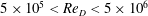
Figure 3. Power curves shown for a single Reynolds number of $Re_{D}=2.82\times 10^{6}$
at various tunnel conditions. Dimensional data are shown in physical units for (a) and then normalized with free-stream conditions for (b). Legend applies to both plots.
$Re_{D}=2.82\times 10^{6}$
at various tunnel conditions. Dimensional data are shown in physical units for (a) and then normalized with free-stream conditions for (b). Legend applies to both plots.

Figure 4. Collapse of data as Reynolds number increases (from (a) to (f)). Data are shown referenced to the tunnel static pressure for convenience (actual density and viscosity calculated at each run condition from measured pressure and temperature).
In addition to achieving dynamic similarity, conducting tests in a pressurized facility comes with a few key advantages. Among them is the ability to match the Reynolds number and tip speed ratio of the full scale using various combinations of dimensional parameters. In the HRTF, multiple experiments were performed at the same Reynolds number but with different tunnel densities and velocities. An example of this method is shown in figure 3. The measured dimensional values of the mean aerodynamic power ( $\unicode[STIX]{x1D70F}\unicode[STIX]{x1D714}$
) as a function of rotational speed (
$\unicode[STIX]{x1D70F}\unicode[STIX]{x1D714}$
) as a function of rotational speed ( $\unicode[STIX]{x1D714}$
) are shown in figure 3(a) for a Reynolds number of
$\unicode[STIX]{x1D714}$
) are shown in figure 3(a) for a Reynolds number of $Re_{D}=2.82\times 10^{6}$
. Tests at this
$Re_{D}=2.82\times 10^{6}$
. Tests at this $Re_{D}$
were performed at four different static pressures as shown. Error bars are shown in shaded grey, and include both systematic and random measurement uncertainties as outlined in § 2.2. In figure 3(b), the same data are shown in non-dimensional form. Since the Reynolds number is kept constant, dynamic similarity implies that the non-dimensional data should collapse to one curve within experimental error. As is evident in figure 3(b), the data exhibit convincing collapse across all values of
$Re_{D}$
were performed at four different static pressures as shown. Error bars are shown in shaded grey, and include both systematic and random measurement uncertainties as outlined in § 2.2. In figure 3(b), the same data are shown in non-dimensional form. Since the Reynolds number is kept constant, dynamic similarity implies that the non-dimensional data should collapse to one curve within experimental error. As is evident in figure 3(b), the data exhibit convincing collapse across all values of $\unicode[STIX]{x1D706}$
, despite the fact that the physical power is nearly doubled from the highest pressure to the lowest pressure case. While these results neatly illustrate the powerful concept of dynamic similarity, they also reflect the high degree of accuracy of the present experimental results. Achieving dynamic similarity at different physical loads also allows for maximizing the accuracy at any given combination of
$\unicode[STIX]{x1D706}$
, despite the fact that the physical power is nearly doubled from the highest pressure to the lowest pressure case. While these results neatly illustrate the powerful concept of dynamic similarity, they also reflect the high degree of accuracy of the present experimental results. Achieving dynamic similarity at different physical loads also allows for maximizing the accuracy at any given combination of $Re$
and
$Re$
and $\unicode[STIX]{x1D706}$
values, since the physical test parameters can be tailored to suit the sensitivity of the measurement equipment, and thus minimize experimental errors.
$\unicode[STIX]{x1D706}$
values, since the physical test parameters can be tailored to suit the sensitivity of the measurement equipment, and thus minimize experimental errors.
Data for $C_{p}$
as a function of
$C_{p}$
as a function of $\unicode[STIX]{x1D706}$
at various values of
$\unicode[STIX]{x1D706}$
at various values of $Re_{D}$
in the range
$Re_{D}$
in the range $0.9\times 10^{6}$
to
$0.9\times 10^{6}$
to $4\times 10^{6}$
are shown in figure 4. Similar to figure 3(b), excellent collapse is seen across a wide range of tunnel conditions at every
$4\times 10^{6}$
are shown in figure 4. Similar to figure 3(b), excellent collapse is seen across a wide range of tunnel conditions at every $Re_{D}$
. For instance, in the case of
$Re_{D}$
. For instance, in the case of $Re_{D}=1.48\times 10^{6}$
in figure 4(b), the operating pressure more than doubles between the datasets shown in black and red coloured markers (and correspondingly, velocity halves), yet the data show excellent agreement for all values of the tip speed ratio. It is useful to note that the error bars decrease in size as
$Re_{D}=1.48\times 10^{6}$
in figure 4(b), the operating pressure more than doubles between the datasets shown in black and red coloured markers (and correspondingly, velocity halves), yet the data show excellent agreement for all values of the tip speed ratio. It is useful to note that the error bars decrease in size as $Re_{D}$
is increased due to the larger magnitude of the actual forces and torques being measured. This directly translates to highly accurate measurements at the highest Reynolds numbers. The plots of figure 4 suggest that any combination of tunnel conditions, which produce a specific
$Re_{D}$
is increased due to the larger magnitude of the actual forces and torques being measured. This directly translates to highly accurate measurements at the highest Reynolds numbers. The plots of figure 4 suggest that any combination of tunnel conditions, which produce a specific $Re_{D}$
, can be chosen to examine
$Re_{D}$
, can be chosen to examine $C_{p}$
.
$C_{p}$
.
3.1 Comparison with FLOWE field data

Figure 5. The power coefficient plotted as a function of tip speed ratio and Reynolds number (given by colour bar). HRTF data are given by crosses while FLOWE field data are shown as a point cloud.
Past work on high-Reynolds-number wind turbines has come almost exclusively from field data. Oftentimes, new research in the wind industry is instigated by observations made in the field. In this regard, a controlled, laboratory experiment such as that presented in this work makes a natural complement to field measurements. It allows for separation of the complicated inflow and unsteady effects in which all real turbines operate to focus on the relevant canonical flow physics driving some observed phenomena.
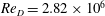
In figure 5, the power coefficient is plotted for various values of $Re_{D}$
and
$Re_{D}$
and $\unicode[STIX]{x1D706}$
. The colour indicates the Reynolds number of a given dataset. Experimental data gathered in the HRTF are shown with crosses connected by solid lines, while field data taken at the FLOWE site for the same turbine geometry are given by the point cloud. Field data points represent averages over 10 min intervals that are individually colour mapped based on the measured Reynolds number. The range of Reynolds numbers shown for the field data is between
$\unicode[STIX]{x1D706}$
. The colour indicates the Reynolds number of a given dataset. Experimental data gathered in the HRTF are shown with crosses connected by solid lines, while field data taken at the FLOWE site for the same turbine geometry are given by the point cloud. Field data points represent averages over 10 min intervals that are individually colour mapped based on the measured Reynolds number. The range of Reynolds numbers shown for the field data is between $740\,000\leqslant Re_{D}\leqslant 2.440\times 10^{6}$
while the experimental data fall between
$740\,000\leqslant Re_{D}\leqslant 2.440\times 10^{6}$
while the experimental data fall between $580\,000\leqslant Re_{D}\leqslant 5\times 10^{6}$
. Overall, the field data report a lower value of the power coefficient for similar Reynolds numbers and tip speed ratios, despite the corrections applied for non-uniform inflow and generator losses. The difference is primarily attributed to uncertainty regarding the exact inflow conditions at the field site. Any small difference in the reference wind velocity (however it is introduced) will cause the power coefficient to scale with the cube of this difference. In addition, free-stream turbulence alone can reduce turbine output power, in some cases by 10 % or more (Sheinman & Rosen Reference Sheinman and Rosen1992). Previous work has measured average values of 26 % at the FLOWE site (Kinzel et al.
Reference Kinzel, Mulligan and Dabiri2012), which is much higher than the nominally laminar (less than 1.1 % turbulence level) inflow of the model. Despite these effects, general trends between both field and laboratory match well, including an increase in
$580\,000\leqslant Re_{D}\leqslant 5\times 10^{6}$
. Overall, the field data report a lower value of the power coefficient for similar Reynolds numbers and tip speed ratios, despite the corrections applied for non-uniform inflow and generator losses. The difference is primarily attributed to uncertainty regarding the exact inflow conditions at the field site. Any small difference in the reference wind velocity (however it is introduced) will cause the power coefficient to scale with the cube of this difference. In addition, free-stream turbulence alone can reduce turbine output power, in some cases by 10 % or more (Sheinman & Rosen Reference Sheinman and Rosen1992). Previous work has measured average values of 26 % at the FLOWE site (Kinzel et al.
Reference Kinzel, Mulligan and Dabiri2012), which is much higher than the nominally laminar (less than 1.1 % turbulence level) inflow of the model. Despite these effects, general trends between both field and laboratory match well, including an increase in $C_{p}$
with
$C_{p}$
with $Re_{D}$
and the region of highest efficiency residing around
$Re_{D}$
and the region of highest efficiency residing around $\unicode[STIX]{x1D706}=1$
.
$\unicode[STIX]{x1D706}=1$
.
The HRTF measurements display an initial, steep gradient in the power coefficient with Reynolds number, suggesting that, even at $Re_{D}$
values matching that of the full scale,
$Re_{D}$
values matching that of the full scale, $C_{p}$
still maintains a strong dependence. The peak power coefficient (
$C_{p}$
still maintains a strong dependence. The peak power coefficient ( $C_{p,max}$
) occurs at a nearly constant tip speed ratio of
$C_{p,max}$
) occurs at a nearly constant tip speed ratio of $\unicode[STIX]{x1D706}=1\pm 0.05$
for all tested Reynolds numbers. The value of
$\unicode[STIX]{x1D706}=1\pm 0.05$
for all tested Reynolds numbers. The value of $Re_{D}$
at which the invariance occurs is lower for higher values of
$Re_{D}$
at which the invariance occurs is lower for higher values of $\unicode[STIX]{x1D706}$
. This observation is due to the fact that the Reynolds number based on the chord length becomes larger as the tip speed ratio is increased.
$\unicode[STIX]{x1D706}$
. This observation is due to the fact that the Reynolds number based on the chord length becomes larger as the tip speed ratio is increased.

Figure 6. Power coefficient as a function of Reynolds number based on diameter and tip speed ratio. HRTF data (black crosses) have been interpolated onto the average operating tip speed ratios for the FLOWE wind turbine (red circles).
To more directly compare the field and laboratory-scale measurements, the FLOWE data were bin-averaged at specific $Re_{D}$
values (which is strongly correlated with
$Re_{D}$
values (which is strongly correlated with $\unicode[STIX]{x1D706}$
in the field) and those resulting data points were used to interpolate HRTF data at specific field operating points. The interpolation of the HRTF data was necessary due to the changing Reynolds number of the field measurements. Figure 6 displays these results for several different
$\unicode[STIX]{x1D706}$
in the field) and those resulting data points were used to interpolate HRTF data at specific field operating points. The interpolation of the HRTF data was necessary due to the changing Reynolds number of the field measurements. Figure 6 displays these results for several different $Re_{D}$
values, along with the associated error bars for each measurement. Despite the difference in overall
$Re_{D}$
values, along with the associated error bars for each measurement. Despite the difference in overall $C_{p}$
(as discussed previously), both datasets exhibit similar trends as Reynolds number increases.
$C_{p}$
(as discussed previously), both datasets exhibit similar trends as Reynolds number increases.
3.2 Reynolds-number invariance
The HRTF data of § 3.1 show a strong dependence on the Reynolds number even when $Re_{D}$
is more than twice the maximum of the field turbine. The invariance of the power coefficient is of particular interest to wind turbine designers and manufacturers, but to the authors’ knowledge has not been studied previously. This section describes the variation of
$Re_{D}$
is more than twice the maximum of the field turbine. The invariance of the power coefficient is of particular interest to wind turbine designers and manufacturers, but to the authors’ knowledge has not been studied previously. This section describes the variation of $C_{p}$
observed in the HRTF experiments and provides support for using the Reynolds number based on the local blade conditions, instead of free-stream values, in order to characterize the observed changes.
$C_{p}$
observed in the HRTF experiments and provides support for using the Reynolds number based on the local blade conditions, instead of free-stream values, in order to characterize the observed changes.

Figure 7. The maximum measured power coefficient shown as a function of Reynolds number based on diameter. Top axis is given in terms of the local blade conditions and taking $\unicode[STIX]{x1D706}=1$
. The crosses are measured data, and the solid line is a fitted error function given by (3.1).
$\unicode[STIX]{x1D706}=1$
. The crosses are measured data, and the solid line is a fitted error function given by (3.1).
Figure 7 shows the peak power coefficient of the HRTF experiments plotted as a function of $Re_{D}$
with the error bars included (note that the errors in
$Re_{D}$
with the error bars included (note that the errors in $Re_{D}$
are smaller than the symbols and were neglected for clarity). The data are also given in terms of the chord Reynolds number along the upper abscissa where a value of
$Re_{D}$
are smaller than the symbols and were neglected for clarity). The data are also given in terms of the chord Reynolds number along the upper abscissa where a value of $\unicode[STIX]{x1D706}=1$
has been used. Here a clear trend is evident, with the power coefficient becoming Reynolds-number-invariant at
$\unicode[STIX]{x1D706}=1$
has been used. Here a clear trend is evident, with the power coefficient becoming Reynolds-number-invariant at $Re_{D}\approx 3\times 10^{6}$
. The line in figure 7 represents a curve fit over a range of
$Re_{D}\approx 3\times 10^{6}$
. The line in figure 7 represents a curve fit over a range of $600\,000\leqslant Re_{D}\leqslant 5\times 10^{6}$
with
$600\,000\leqslant Re_{D}\leqslant 5\times 10^{6}$
with
 $$\begin{eqnarray}C_{p,max}=0.1444\,\text{erf}(0.5133\times 10^{-6}\,Re_{D})+0.1128,\end{eqnarray}$$
where $\text{erf}$
is the error function. This scaling can be used to guide experimental design when determining the conditions necessary to achieve Reynolds-number independence, or possibly even interpreting data acquired at low Reynolds numbers. In the lens of the FLOWE field data, this can be viewed as the asymptotic state for a field turbine operating in the ideal case of steady, laminar inflow conditions at high Reynolds number.
$\text{erf}$
is the error function. This scaling can be used to guide experimental design when determining the conditions necessary to achieve Reynolds-number independence, or possibly even interpreting data acquired at low Reynolds numbers. In the lens of the FLOWE field data, this can be viewed as the asymptotic state for a field turbine operating in the ideal case of steady, laminar inflow conditions at high Reynolds number.
As expected, and as demonstrated previously in figure 5, the power coefficient reaches a different asymptotic value depending on the tip speed ratio. Each value of $\unicode[STIX]{x1D706}$
therefore has a maximum
$\unicode[STIX]{x1D706}$
therefore has a maximum $C_{p}$
, which is achieved if the Reynolds number is large enough. This was clearly demonstrated in figure 7 for
$C_{p}$
, which is achieved if the Reynolds number is large enough. This was clearly demonstrated in figure 7 for $\unicode[STIX]{x1D706}=1$
when
$\unicode[STIX]{x1D706}=1$
when $Re_{D}$
exceeded a value of
$Re_{D}$
exceeded a value of $3\times 10^{6}$
. This two-parameter dependence indicates that a single non-dimensional group, the previously discussed Reynolds number based on chord length,
$3\times 10^{6}$
. This two-parameter dependence indicates that a single non-dimensional group, the previously discussed Reynolds number based on chord length, $Re_{c}$
, would more accurately capture the behaviour of the power coefficient. It includes both the outer-flow effects of
$Re_{c}$
, would more accurately capture the behaviour of the power coefficient. It includes both the outer-flow effects of $Re_{D}$
and information on the local blade conditions given by
$Re_{D}$
and information on the local blade conditions given by $\unicode[STIX]{x1D706}$
. To investigate this claim, the data of figure 5 have been interpolated to a specified grid of tip speed ratios, allowing for direct comparison across datasets. The resulting points are shown in figure 8(a) as a function of
$\unicode[STIX]{x1D706}$
. To investigate this claim, the data of figure 5 have been interpolated to a specified grid of tip speed ratios, allowing for direct comparison across datasets. The resulting points are shown in figure 8(a) as a function of $Re_{c}$
. Note that the
$Re_{c}$
. Note that the $\unicode[STIX]{x1D706}=1$
points are identical to figure 7. Above
$\unicode[STIX]{x1D706}=1$
points are identical to figure 7. Above $Re_{c}=1.5\times 10^{6}$
, the HRTF data become invariant to additional increases in blade Reynolds number, regardless of the
$Re_{c}=1.5\times 10^{6}$
, the HRTF data become invariant to additional increases in blade Reynolds number, regardless of the $\unicode[STIX]{x1D706}$
chosen. The mean value of the power coefficient above this threshold is denoted by
$\unicode[STIX]{x1D706}$
chosen. The mean value of the power coefficient above this threshold is denoted by $C_{p,\infty }$
.
$C_{p,\infty }$
.
The data of figure 8(a) also indicate that a specific value of $C_{p,\infty }$
exists for each
$C_{p,\infty }$
exists for each $\unicode[STIX]{x1D706}$
, which may be found by averaging
$\unicode[STIX]{x1D706}$
, which may be found by averaging $C_{p}$
above the invariance threshold of
$C_{p}$
above the invariance threshold of $Re_{c}=1.5\times 10^{6}$
. Then
$Re_{c}=1.5\times 10^{6}$
. Then $C_{p,\infty }$
for each specific
$C_{p,\infty }$
for each specific $\unicode[STIX]{x1D706}$
is used to normalize the entire curve, ideally showing an asymptote to a value of 1 as
$\unicode[STIX]{x1D706}$
is used to normalize the entire curve, ideally showing an asymptote to a value of 1 as $Re_{c}$
crosses the threshold value. This is shown in figure 8(b) with excellent collapse across the entire range of
$Re_{c}$
crosses the threshold value. This is shown in figure 8(b) with excellent collapse across the entire range of $C_{p}$
and
$C_{p}$
and $\unicode[STIX]{x1D706}$
values.
$\unicode[STIX]{x1D706}$
values.

Figure 8. Power coefficient shown as a function of the blade Reynolds number in (a). Data have been interpolated to a fixed $\unicode[STIX]{x1D706}$
grid as given by the legend of (b). (b) These same data normalized by the Reynolds-number-invariant value of
$\unicode[STIX]{x1D706}$
grid as given by the legend of (b). (b) These same data normalized by the Reynolds-number-invariant value of $C_{p}$
, found as the mean power coefficient for cases where
$C_{p}$
, found as the mean power coefficient for cases where $Re_{c}>1.5\times 10^{6}$
. Legend applies to both plots.
$Re_{c}>1.5\times 10^{6}$
. Legend applies to both plots.
The final value of $C_{p,\infty }$
can be plotted against its respective tip speed ratio to produce the invariant power coefficient curve as in figure 9. This curve represents the asymptotic operational state of the WPE vertical-axis wind turbine used in this study. Experiments and simulations using this geometry will return points on this curve if the blade Reynolds number is above the threshold value of
$C_{p,\infty }$
can be plotted against its respective tip speed ratio to produce the invariant power coefficient curve as in figure 9. This curve represents the asymptotic operational state of the WPE vertical-axis wind turbine used in this study. Experiments and simulations using this geometry will return points on this curve if the blade Reynolds number is above the threshold value of $Re_{c}=1.5\times 10^{6}$
.
$Re_{c}=1.5\times 10^{6}$
.

Figure 9. Reynolds-number-invariant power coefficient as a function of tip speed ratio. Symbols as in figure 8.
4 Conclusions
A new methodology for investigating high-Reynolds-number rotating flows is introduced. By using a high-density working fluid, relatively low velocities and geometrically similar test models, dynamic similarity is achieved for a commercially available vertical-axis wind turbine. The experimental campaign investigated a flow regime that was previously unavailable to those in the wind turbine aerodynamics community. The power coefficient of a model turbine was measured over an entire decade of Reynolds numbers, from $5\times 10^{5}$
to
$5\times 10^{5}$
to $5\times 10^{6}$
, which exceeds the Reynolds number to which the full-scale turbine is exposed in the field. The strength of dynamic similarity and the accuracy of the measurements were demonstrated for various Reynolds numbers and over a realistic range of tip speed ratios, by varying the testing conditions. The model turbine data exhibit excellent collapse for distinct Reynolds numbers, with all data points falling well within experimental error. The maximum power coefficient was found to occur at a nearly constant
$5\times 10^{6}$
, which exceeds the Reynolds number to which the full-scale turbine is exposed in the field. The strength of dynamic similarity and the accuracy of the measurements were demonstrated for various Reynolds numbers and over a realistic range of tip speed ratios, by varying the testing conditions. The model turbine data exhibit excellent collapse for distinct Reynolds numbers, with all data points falling well within experimental error. The maximum power coefficient was found to occur at a nearly constant $\unicode[STIX]{x1D706}=1$
regardless of the tested Reynolds number in both laboratory and field experiments. It was found that the power coefficient becomes Reynolds-number-invariant above a critical Reynolds number. Furthermore, the critical Reynolds number was found to be
$\unicode[STIX]{x1D706}=1$
regardless of the tested Reynolds number in both laboratory and field experiments. It was found that the power coefficient becomes Reynolds-number-invariant above a critical Reynolds number. Furthermore, the critical Reynolds number was found to be $Re_{c}=1.5\times 10^{6}$
, independent of the specific
$Re_{c}=1.5\times 10^{6}$
, independent of the specific $Re_{D}$
or
$Re_{D}$
or $\unicode[STIX]{x1D706}$
chosen. Finally, the invariant power curve was produced using this threshold value on Reynolds number with the results having direct impact on efforts to model and simulate the flow physics of vertical-axis wind turbines.
$\unicode[STIX]{x1D706}$
chosen. Finally, the invariant power curve was produced using this threshold value on Reynolds number with the results having direct impact on efforts to model and simulate the flow physics of vertical-axis wind turbines.
Acknowledgements
The support of the National Science Foundation under grants CBET-1435254 and CBET-1652583 as well as the Gordon and Betty Moore Foundation under grant 2645 is gratefully acknowledged. The authors also wish to thank L. Tang and S. Sudhakar for assisting with the design and manufacture of the wind turbine model.


