


1. Introduction
Electrophoresis is an electrokinetic phenomenon, in which a charged colloidal particle suspended in an electrolyte is set in motion by an applied electric field. Electrophoresis has applications in colloid science (Russel, Saville & Schowalter Reference Russel, Saville and Schowalter1991), microfluidics (Erickson & Li Reference Erickson and Li2004; Liu & Mathies Reference Liu and Mathies2009), DNA sequencing (Huang, Quesada & Mathies Reference Huang, Quesada and Mathies1992), protein separation (Zhu, Lu & Liu Reference Zhu, Lu and Liu2012), active matter (De Corato et al. Reference De Corato, Arqué, Patino, Arroyo, Sánchez and Pagonabarraga2020) and directed assembly (Mittal et al. Reference Mittal, Lele, Kaler and Furst2008), among others. The strength of the imposed electric field is characterized by the dimensionless parameter  $\beta =a^*e^*E_\infty ^*/k_B^*T^*$, for a spherical particle of radius $a^*$ in a monovalent electrolyte under an applied electric field with magnitude $E_\infty ^*$. Here, $k_B^*T^*/e^*$ is the thermal voltage, where $k_B^*$ is the Boltzmann constant, $T^*$ is the absolute temperature, and $e^*$ is the elementary charge. For reference, the thermal voltage is approximately $25\ \mathrm {mV}$ at $T^*=298\ \mathrm {K}$. Variables decorated by an asterisk are dimensional quantities. Other useful parameters to characterize different regimes in electrophoresis are the dimensionless Debye layer thickness $\delta =1/(\kappa ^*a^*)$ and the dimensionless surface charge density $\sigma =e^*a^*\sigma ^*/\epsilon ^*k_B^*T^*$. Here, $1/\kappa ^*$ is the Debye length, $\sigma ^*$ is the dimensional surface charge density, and $\epsilon ^*$ is the fluid permittivity. For example, the thin-Debye-layer limit, $\delta \ll 1$, is relevant to micron-sized colloidal particles in aqueous electrolytes at millimolar (and higher) concentrations. Here, Schnitzer & Yariv (Reference Schnitzer and Yariv2012b) define $\sigma ={O}(1)$ as a moderately charged particle, and $\sigma ={O}(\delta ^{-1})$ as a highly charged particle.
Initial developments on the theory of electrophoresis were made by Smoluchowski (Reference Smoluchowski1903), who formulated his famous equation
 \begin{equation} \boldsymbol{U}^*=\frac{\epsilon^*\zeta^*\boldsymbol{E}_{\infty}^*}{\eta^*}, \end{equation}
which establishes a linear relation between the steady electrophoretic velocity  $\boldsymbol {U}^*$ of the particle and the imposed (steady, uniform) electric field $\boldsymbol {E}_\infty ^*$, where $\zeta ^*$ is the zeta potential of the colloid in a given electrolytic solution, and $\eta ^*$ is the dynamic viscosity of the fluid. Smoluchowski's equation is valid when the Debye length is small compared to the particle size, and for moderately charged particles, $\sigma ={O}(1)$. An equivalent expression for a fixed surface charge on the particle is
 \begin{equation} \boldsymbol{U}^*=\frac{\sigma^*\boldsymbol{E}_{\infty}^*}{\kappa^*\eta^*}, \end{equation}
in which case it is evident that the electrophoretic velocity is asymptotically small in the thin-Debye-layer limit. Furthermore, Smoluchowski's derivation of this equation assumes the weak-field limit,  $\beta \ll 1$. Further developments by Debye & Hückel (Reference Debye and Hückel1924) for thick Debye layers, $\delta \gg 1$, and Henry (Reference Henry1931) for arbitrary $\delta$, also found linear relations between the particle velocity and the applied electric field, since these too assumed the weak-field limit. Specifically, the Hückel result in terms of charge density is
 \begin{equation} \boldsymbol{U}^*=\frac{2a^*\sigma^*\boldsymbol{E}_{\infty}^*}{3\eta^*}. \end{equation}
 Overbeek (Reference Overbeek1943) and Booth (Reference Booth1950) included ionic convection in the electrokinetic model for electrophoresis, which accounts for relaxation effects that arise due to a relative motion between the colloid and the ions, albeit only for moderately charged particles. Numerical results by Wiersema, Loeb & Overbeek (Reference Wiersema, Loeb and Overbeek1966) and O'Brien & White (Reference O'Brien and White1978), including retardation and relaxation effects for highly charged particles, followed. Here, by ‘relaxation’ we refer to deformation of the charge cloud from its spherically symmetric equilibrium state, and by ‘retardation’ we refer to a reduction in the electrophoretic speed in comparison to Smoluchowski's result. These works showed, in particular, that the electrophoretic velocity does not remain a linear function of the zeta potential for particles of sufficiently high surface charge in the weak-field limit. In the thin-Debye-layer regime, this deviation from linearity can be interpreted as being caused by surface conduction of ions in the Debye layer. Indeed, perturbation analyses by Dukhin & Semenikhin (Reference Dukhin and Semenikhin1970) and O'Brien & Hunter (Reference O'Brien and Hunter1981) allowed for a correction to Smoluchowski's formula in binary electrolytes for thin Debye layers, owing to surface conduction; this was later generalized to multi-component electrolytes by O'Brien (Reference O'Brien1983). However, just as in the earlier developments in the theory of electrophoresis, the focus remained in the weak-field regime,  $\beta \ll 1$, where the particle velocity remains linear in electric field strength.
An asymptotic analysis for nonlinear electrophoretic motion of highly charged particles in the thin-Debye-layer limit  $(\delta \ll 1)$ was developed by Schnitzer & Yariv (Reference Schnitzer and Yariv2012b). Here, by nonlinear electrophoresis we refer to conditions where $\beta$ is not much smaller than unity, i.e. beyond the weak-field limit. Specifically, they created a macroscale model for moderate electric fields, corresponding to $\beta ={O}(1)$, wherein the Debye-scale transport is coarse-grained into effective boundary conditions on the equations governing the electrostatic potential and neutral salt concentration in the electroneutral bulk electrolyte outside the Debye layer. The potential and salt evolution in the bulk is also coupled to bulk fluid flow via the Stokes equations with a Coulomb body force. Using this macroscale model, they calculated the electrophoretic velocity of a spherical particle in the ‘weakly nonlinear regime’ as a perturbation expansion in $\beta$ (Schnitzer et al. Reference Schnitzer, Zeyde, Yavneh and Yariv2013), for $\sigma ={O}(\delta ^{-1})$ and arbitrary Dukhin number $Du$. The latter quantity is a measure of the surface conductivity relative to bulk conductivity, and is defined as
 \begin{equation} Du=\delta^2\sigma(1+2\alpha^-), \end{equation}
in which  $\alpha ^-$ is the counterion drag coefficient. The difference between our definition of $Du$ and the one given by Schnitzer et al. (Reference Schnitzer, Zeyde, Yavneh and Yariv2013) lies in the different normalization of the surface charge density. In this weakly nonlinear regime, they found that the first nonlinear contribution to the electrophoretic velocity is of order $\beta ^3$. In a subsequent paper (Schnitzer & Yariv Reference Schnitzer and Yariv2014), they analysed their macroscale model at small $Du$ across the transition from weak to strong fields. Here, the field dependence of the nonlinear electrophoretic velocity is parametrized via the Péclet number $Pe=\alpha \zeta _0\beta$, which physically represents the relative importance of ion advection to diffusion; $\alpha$ is the mean ionic drag coefficient, and $\zeta _0$ is the dimensionless equilibrium zeta potential (normalized by the thermal voltage), defined via
 \begin{equation} \sigma=2\delta^{{-}1}\sinh(\zeta_0/2). \end{equation}
The nonlinear electrophoretic velocity scales as  $\beta ^3$ at small $Pe$, and as $\beta ^{3/2}$ at large $Pe$. While analytical results are not available in the transition between these two regimes, numerical computations suggest a smooth transition of the electrophoretic velocity between these limiting cases.
Experiments on nonlinear electrophoresis have confirmed that the electrophoretic velocity has a nonlinear dependence on the field strength at sufficiently large applied fields. Tottori et al. (Reference Tottori, Misiunas, Keyser and Bonthuis2019) conducted experiments, as well as COMSOL simulations, involving highly charged submicron particles in the weakly nonlinear regime: their results are in good agreement with Schnitzer et al. (Reference Schnitzer, Zeyde, Yavneh and Yariv2013). Cardenas-Benitez et al. (Reference Cardenas-Benitez, Jind, Gallo-Villanueva, Martinez-Chapa, Lapizco-Encinas and Perez-Gonzalez2020) performed experiments in direct current (DC) insulator-based dielectrophoresis microfluidic devices, and attributed the observed reversal of the particle velocity direction when subjected to strong DC fields to a nonlinear electrophoretic mobility, instead of dielectrophoretic effects. Antunez-Vela et al. (Reference Antunez-Vela, Perez-Gonzalez, De Peña, Lentz and Lapizco-Encinas2020) used this set-up to determine experimentally the field strength at which the electrophoretic particle velocity balances particle advection due to electro-osmotic flow in the microchannel, resulting in particle trapping. Kumar et al. (Reference Kumar, Elele, Yeksel, Khusid, Qiu and Acrivos2006) developed a microfluidic technique to measure the electrophoretic velocity at large field strengths; in contrast to the above-mentioned studies, their results show the linear theory of electrophoresis extends beyond the weak-field regime in the case of moderately charged particles. This is in line with Schnitzer & Yariv (Reference Schnitzer and Yariv2012b), who demonstrated that Smoluchowski's formula is indeed valid at  $\beta ={O}(1)$ for moderately charged particles. In fact, these authors in an earlier work (Schnitzer & Yariv Reference Schnitzer and Yariv2012c) demonstrated that Smoluchowski's formula holds until strong fields, where $\beta ={O}(\delta ^{-1})$. This last conclusion, however, could be invalidated by consideration of dielectric–solid polarization at strong fields (Schnitzer & Yariv Reference Schnitzer and Yariv2012a).
Theoretical and numerical results for nonlinear electrophoresis beyond the thin-Debye-layer limit are relatively scarce. Khair (Reference Khair2018) developed an asymptotic approximation to the nonlinear electrophoretic velocity for weakly charged colloids  ${(\sigma \ll 1)}$ with thick Debye layers $(\delta \gg 1)$. It was predicted that in the strong-field regime, the electrophoretic velocity approaches Hückel's result as the Debye cloud is stripped from the particle at large $\beta$. Interestingly, the notion of Debye cloud stripping was suggested by Stotz (Reference Stotz1978) in his experimental study of nonlinear electrophoresis in a non-polar fluid. Numerical computations from Fixman & Jagannathan (Reference Fixman and Jagannathan1983), using a multipole expansion to solve the full electrokinetic equations, showed no nonlinear dependence of the electrophoretic velocity on field strength at $\beta ={O}(1)$ for particles with $\zeta ^*={O}(k_B^*T^*/e^*)$. Computations from Bhattacharyya & Gopmandal (Reference Bhattacharyya and Gopmandal2011) for the hydrodynamic drag force on a charged particle exhibited a nonlinear dependence on field strength, at sufficiently large fields. Numerical results from Frants et al. (Reference Frants, Artyukhov, Kireeva, Ganchenko and Demekhin2021) in the thin-Debye-layer limit suggested a transition to an unsteady, and eventually chaotic, flow in very strong steady fields, i.e. $\beta \gg 1$, due to the formation of unstable microvortices, which lose their steadiness as the electric field increases.
In general, the nonlinear coupling between the ion concentration, the electric field and the fluid flow around the particle means that a numerical scheme must be used to compute nonlinear electrophoresis outside the weak-field regime for arbitrary Debye lengths. In the present work, a robust numerical scheme, employing a spectral element method algorithm, is developed to compute the electrophoretic velocity of a spherical, dielectric, rigid, uniformly charged particle immersed in a monovalent electrolyte for, in principle, arbitrary Debye lengths and electric field magnitudes. Additionally, the permittivity of the particle is assumed to be small compared to that of the electrolyte, which obviates the need to determine the electric potential variation within the particle. Note that this assumption is reasonable for colloidal particles of inorganic composition (e.g. silica or polystyrene) in aqueous solutions. The following sections are structured as follows. In § 2, the electrokinetic governing equations and the model assumptions are introduced. In § 3, the numerical scheme is described. In § 4, results for moderately charged and highly charged particles are presented, wherein comparisons between the present work and previous theoretical and experimental studies are made. Finally, in § 5, we offer concluding remarks and suggestions for future work.
2. Problem formulation
Consider a spherical colloidal particle freely suspended in a monovalent electrolyte solution, as shown in figure 1. Depending on the physico-chemical nature of the colloid–electrolyte interface, the particle may acquire a non-zero charge on its surface at equilibrium. To compensate this surface charge, an ion cloud richer in counterions will form around the colloid. This so-called Debye cloud, or layer, is characterized by a thickness, the Debye length  $1/\kappa ^*=\sqrt {\epsilon ^*k_B^*T^*/2(e^*)^2c_\infty ^*}$, where $c_\infty ^*$ is the bulk electrolyte concentration far from the particle. For example, $1/\kappa ^*$ is approximately $10\ \mathrm {nm}$ for a $1\ \mathrm {mM}$ aqueous solution of a monovalent electrolyte at $298\ \mathrm {K}$. Normalizing this Debye length by the particle radius $a^*$ results in the dimensionless Debye layer thickness $\delta =1/(\kappa ^*a^*)$. For an isothermal system, $\delta$ is a function of only the particle radius and the bulk electrolyte concentration. Thin Debye layers ( $\delta \ll 1$) are present in the case of large colloids or highly concentrated electrolytes. In contrast, when the colloids are small or in case of diluted solutions, this corresponds to the thick Debye layer ( $\delta \gg 1$) regime. If an electric field with dimensionless strength $\beta$ is imposed, then the colloid will move at a speed $U$ along the same axis as the applied electric field. Here, $U=(e^*/k_B^*T^*)^2\eta ^*a^*U^*/\epsilon ^*$ is the dimensionless electrophoretic speed, and $U^*$ is its dimensional form. From figure 1, the surface charge is depicted as positive without loss of generality; therefore the cations and anions correspond to the coions and counterions, respectively.

Figure 1. Diagram of a colloidal particle with positive surface charge density  $\sigma$ and a Debye layer of thickness $\delta$ suspended in an electrolyte, moving at electrophoretic speed $U$, under the influence of an applied electric field with dimensionless strength $\beta$. The main goal is to calculate $U$ with prescribed values of $\delta$, $\sigma$ and $\beta$.
To determine  $U$, one must solve the electrokinetic equations, which encompass coupled fluid flow, ion transport and electric fields. Since we are interested in the steady-state particle velocity, we disregard the time dependence in these governing equations. Changes in temperature that would lead to variations in the physical properties of the electrolyte are neglected. Thus the system is isothermal and time-invariant. The governing equations will be presented in dimensionless form. The electric potential, ion concentration and velocity are normalized by the factors $k_B^*T^*/e^*$, $c_\infty ^*$ and $\epsilon ^*(k_B^*T^*/e^*)^2/\eta ^*a^*$, respectively, while the pressure and stress tensors are normalized by the Maxwell scale $\epsilon ^*(k_B^*T^*/a^*e^*)^2$.
The conditions under which colloidal electrophoresis occurs correspond to an electro-quasi-static regime, meaning that all induced magnetic effects can be neglected safely. Hence the electric field in the electrolyte is governed by the Poisson equation
 \begin{equation} \delta^2\,\nabla^2\varphi={-}\tfrac{1}{2}(c^+-c^-), \end{equation}
where  $\varphi$ is the dimensionless electric potential and $c^\pm$ stands for the dimensionless ion concentration, with the positive (negative) sign for cations (anions). The right-hand side of (2.1) represents the negative of the ionic charge density. The fluid flow is governed by the continuity and Stokes equations,
 $$\begin{gather} \boldsymbol{\nabla}\boldsymbol{\cdot}\boldsymbol{u}=0, \end{gather}$$
 $$\begin{gather}-\boldsymbol{\nabla}p+\nabla^2\boldsymbol{u}-\frac{c^+-c^-}{2\delta^2}\,\boldsymbol{\nabla}\varphi=\boldsymbol{0}, \end{gather}$$
where  $\boldsymbol {u}$ is the dimensionless fluid velocity field and $p$ is the dimensionless pressure. Equation (2.3) excludes the inertia term; this is valid as long as the Reynolds number is small, which is a plausible assumption for micron-scale colloidal particles in aqueous solutions, moving at speeds less than approximately $1\ \mathrm {cm}\ \mathrm {s}^{-1}$. The last term in (2.3) is the Coulomb body force that acts on any non-electroneutral fluid element.
The ion concentration is governed by the stationary ion mass balance, i.e. the steady-state Nernst–Planck equations
 \begin{equation} \nabla^2c^\pm\pm\boldsymbol{\nabla}\boldsymbol{\cdot}(c^\pm\,\boldsymbol{\nabla}\varphi)-\alpha^\pm \boldsymbol{u}\boldsymbol{\cdot}\boldsymbol{\nabla}c^\pm=0. \end{equation}
 The three terms in (2.4) represent, from left to right, diffusion, electromigration and advection, respectively. The parameter  $\alpha ^\pm =\epsilon ^*(k_B^*T^*/e^*)^2/D^\pm \eta ^*$ is the ion drag coefficient, where $D^\pm$ is the ion diffusion coefficient. Values of $\alpha ^\pm$ in an aqueous solution at $298\ \mathrm {K}$ are in the range 0.1–2 for most common systems (Vanysek Reference Vanysek1993).
For application of the boundary conditions, it is convenient to work in a reference frame that translates with the particle speed  $U$. In this case, the particle is stationary, and the fluid far from the particle moves at speed $-U$. We assume that the surface charge distribution on the colloid remains fixed as the imposed electric field varies in magnitude. Therefore, the inner boundary condition for the electric potential corresponds to the Gauss law at the colloid surface,
 \begin{equation} \boldsymbol{n}\boldsymbol{\cdot}\boldsymbol{\nabla}\varphi={-}\sigma\quad \text{at} \ r=1, \end{equation}
where  $\boldsymbol {n}$ is an outward unit vector normal to the colloid surface, and $r$ is the radial distance in spherical coordinates with origin at the centre of the colloid. We neglect the electric field variation inside the colloid in (2.5) due to the assumed small ratio of particle to fluid permittivity.
For the fluid flow problem we assume no-slip, and for the Nernst–Planck equations we impose the no-flux condition through the colloid, namely,
 \begin{equation} \boldsymbol{u}=\boldsymbol{0}\quad \text{and}\quad \boldsymbol{n}\boldsymbol{\cdot}[\boldsymbol{\nabla}c^\pm\pm c^\pm\,\boldsymbol{\nabla}\varphi]=0 \quad \text{at}\ r=1. \end{equation}
The advection term in (2.4) does not contribute to the no-flux condition in the co-moving reference frame because of the no-slip condition.
Far from the colloid, the electric field tends to the imposed electric field  $\boldsymbol {E}_\infty$, and the ion concentration must be equal to the bulk concentration $c_\infty$ to satisfy electroneutrality at the bulk. In dimensionless form, we have
 \begin{equation} \boldsymbol{\nabla}\varphi\to-\beta\hat{\boldsymbol{z}} \quad \text{and}\quad c^\pm\to 1\quad \text{as}\ r\to\infty, \end{equation}
where  $\hat {\boldsymbol {z}}$ denotes the unit vector corresponding to the axis in which the electric field is applied. Since the reference frame is moving with the colloid, the far-field boundary condition for the flow problem is
 \begin{equation} \boldsymbol{u}\to-U\hat{\boldsymbol{z}}\quad \text{as}\ r\to\infty, \end{equation}
where  $U$ is the electrophoretic speed. This value is unknown a priori; in fact, it is the main goal of the calculation. Since the system is at steady state, we find $U$ by enforcing zero net force on the particle:
 \begin{equation} \oint_S(\boldsymbol{\mathsf{N}}+\boldsymbol{\mathsf{M}})\boldsymbol{\cdot}\boldsymbol{n}\,{\rm d}S=\boldsymbol{0}, \end{equation}
where  $\boldsymbol{\mathsf{N}}$ and $\boldsymbol{\mathsf{M}}$ are the dimensionless hydrodynamic and Maxwell stress tensors, respectively, i.e.
 $$\begin{gather} \boldsymbol{\mathsf{N}}={-}p\boldsymbol{\mathsf{I}}+[\boldsymbol{\nabla} \boldsymbol{u}+(\boldsymbol{\nabla} \boldsymbol{u})^{\rm T}], \end{gather}$$
 $$\begin{gather}\boldsymbol{\mathsf{M}}=\boldsymbol{\nabla}\varphi\,\boldsymbol{\nabla}\varphi-\tfrac{1}{2}(\boldsymbol{\nabla} \varphi\boldsymbol{\cdot}\boldsymbol{\nabla}\varphi)\boldsymbol{\mathsf{I}}. \end{gather}$$
Here,  $\boldsymbol{\mathsf{I}}$ denotes the identity tensor, and the superscript ${\rm T}$ denotes the transpose. By applying the divergence theorem to (2.9), we see that $\boldsymbol{\mathsf{N}}+\boldsymbol{\mathsf{M}}$ must be divergence-free, therefore $S$ in (2.9) is an arbitrary surface of integration enclosing the particle; we choose the particle surface $r=1$ as $S$.
$S$.
The nonlinearity in the governing equations stemming from the Coulomb force in (2.3), and the electromigration and advection terms in (2.4), as well as electromigration in the no-flux boundary condition, means that a numerical approach is generally necessary to explore the regimes of nonlinear electrophoresis.
3. Numerical formulation
Our numerical approach to find the electrophoretic speed of the particle proceeds in two steps. First, a solution of the electrokinetic equations is found, given a guess of the electrophoretic speed, by employing a spectral element method algorithm, adapted from Chisholm et al. (Reference Chisholm, Legendre, Lauga and Khair2016). Then the electrophoretic speed is computed by imposing (2.9), given a solution for  $\varphi$, $c^\pm$ and $\boldsymbol {u}$ from the previous step in the system domain. The final solution is found by performing these two steps iteratively until convergence is reached within a prescribed tolerance.
The first step is solved by employing a spectral element method approach and the Galerkin method of weighted residuals (Karniadakis & Sherwin Reference Karniadakis and Sherwin2005). This requires the use of high-order polynomials for both the trial and test functions to achieve the desired spectral convergence. In addition, both trial and test spaces must be equal for the Galerkin method. The two-dimensional basis set is defined as a tensor product of one-dimensional Lagrange polynomials of order  $N$, which leads to $(N+1)^2$ degrees of freedom for each element. Finally, Gauss–Lobatto quadrature is employed to integrate over each parametric $[-1, 1]^2$ subdomain. The reader is referred to Chisholm et al. (Reference Chisholm, Legendre, Lauga and Khair2016) for more details of this numerical approach.
Due to the geometry of the system, we can benefit from the symmetry around the axis of the applied field; the azimuthal dependence of the variables involved is dropped, and the model is simplified to an axisymmetric two-dimensional problem. By exploiting this feature, (2.2) and (2.3) can be cast into the more convenient vorticity–streamfunction formulation:
 $$\begin{gather} E^2\psi+\omega=0, \end{gather}$$
 $$\begin{gather}2\delta^2\,\nabla^2\boldsymbol{\omega}-\boldsymbol{\nabla}(c^+-c^-)\times\boldsymbol{\nabla}\varphi=\boldsymbol{0}, \end{gather}$$
in which  $\boldsymbol {\omega }=\boldsymbol {\nabla }\times \boldsymbol {u}$ is the vorticity field, $\omega$ is its azimuthal (and only non-zero) component, $\psi$ is the streamfunction, and $E^2$ is a second-order differential operator. In cylindrical coordinates $(z,\rho )$, in which $z$ corresponds to the symmetry axis and $\rho$ is the normal distance to this axis, $E^2$ is defined as
 \begin{equation} E^2=\frac{1}{\rho}\left(\frac{\partial^2}{\partial\rho^2}-\frac{1}{\rho}\,\frac{\partial}{\partial\rho}+\frac{\partial^2}{\partial z^2}\right). \end{equation}
 The relation between the streamfunction  $\psi$ and the velocity field $\boldsymbol {u}$ in cylindrical coordinates is given by
 \begin{equation} \boldsymbol{u}=\frac{1}{\rho}\left(\frac{\partial\psi}{\partial\rho}\,\hat{\boldsymbol{z}}-\frac{\partial\psi}{\partial z}\,\hat{\boldsymbol{\rho}}\right), \end{equation}
where  $\hat {\boldsymbol {\rho }}$ is the unit vector normal to the axis of symmetry. A cylindrical coordinates system is selected to facilitate the transition to the Cartesian parametric space. The singularity at the symmetry axis introduced by this coordinate system can be circumvented with Dirichlet boundary conditions for $\psi$ at the symmetry axis. The flow boundary conditions (2.6) and (2.8) in the vorticity–streamfunction formulation become
 $$\begin{gather} \psi=A\quad\text{at}\ r=1, \end{gather}$$
 $$\begin{gather}\omega\to 0\quad \text{as}\ r\to\infty, \end{gather}$$
 $$\begin{gather}\boldsymbol{n}\boldsymbol{\cdot}\boldsymbol{\nabla}\psi\to -U\rho\sin\theta\quad \text{as}\ r\to\infty, \end{gather}$$
where  $A$ is an arbitrary constant; $A=0$ is chosen for convenience.
By taking the inner product of (2.1), (2.4), (3.1) and (3.2) with the test functions  $\phi$, we obtain the weak formulation of the full electrokinetic equations:
 $$\begin{gather} 2\delta^2\left[\langle\boldsymbol{\nabla}\phi,\boldsymbol{\nabla}\varphi\rangle-\left\langle\phi,\boldsymbol{n} \boldsymbol{\cdot}\boldsymbol{\nabla}\varphi\right\rangle_\partial\right]-\langle\phi,c^+-c^-\rangle=0, \end{gather}$$
 $$\begin{gather}\left\langle\boldsymbol{\nabla}\phi,\boldsymbol{\nabla} c^\pm\pm c^\pm\,\boldsymbol{\nabla}\varphi-\frac{\alpha^\pm}{\rho}\, c^\pm\,\boldsymbol{\nabla}^\bot\psi\right\rangle-\left\langle\phi,\boldsymbol{n} \boldsymbol{\cdot}\left(\boldsymbol{\nabla}c^\pm\pm c^\pm\,\boldsymbol{\nabla}\varphi-\frac{\alpha^\pm}{\rho}\,c^\pm\,\boldsymbol{\nabla}\psi\right)\right\rangle_\partial=0, \end{gather}$$
 $$\begin{gather}\langle\boldsymbol{\nabla}\phi,\boldsymbol{\nabla}\psi\rangle+\left\langle\phi,\frac{2}{\rho}\,\frac{\partial\psi}{ \partial\rho}-\rho\omega\right\rangle-\left\langle\phi,\boldsymbol{n} \boldsymbol{\cdot}\boldsymbol{\nabla}\psi\right\rangle_\partial=0, \end{gather}$$
 $$\begin{gather}2\delta^2\left[\langle\boldsymbol{\nabla}\phi,\boldsymbol{\nabla}\omega\rangle+\frac{1}{ \rho^2}\,\langle\phi,\omega\rangle-\left\langle\phi,\boldsymbol{n}\boldsymbol{\cdot} \boldsymbol{\nabla}\omega\right\rangle_\partial\right]+\langle\phi,\boldsymbol{\nabla}(c^+-c^-) \times\boldsymbol{\nabla}\varphi\rangle=0. \end{gather}$$
Here, the angle brackets denote the inner product. Equations (3.8)–(3.11) correspond to the Poisson, Nernst–Planck, vorticity definition and vorticity transport equations, respectively, in cylindrical coordinates. The subscript  $\partial$ denotes a boundary integral, which is evaluated only at the particle surface, the axis of symmetry and the boundary far from the particle. The second-order terms are converted to first order plus a boundary term by integrating by parts and making use of the divergence theorem.
Direct implementation of (3.8)–(3.11) would result in unnecessary computation at each step. To alleviate this issue, we define operators that can be fully defined once at the beginning of the computation, namely,  $\mathbb {M}_{ij}=\langle H_i,H_j\rangle$, $\mathbb {L}_{ij}=\langle \boldsymbol {\nabla } H_i,\boldsymbol {\nabla } H_j\rangle$, $\mathbb {B}_{ijk}=\langle H_i,H_j\,\boldsymbol {\nabla } H_k\rangle$, $\mathbb {D}_{ijk}=\langle H_i,\boldsymbol {\nabla } H_j\times \boldsymbol {\nabla } H_k\rangle$, $\mathbb{L}_{ij}^V=\mathbb {L}_{ij}+\langle H_i,H_j\rangle /\rho ^2$, $\mathbb {A}_{ijk}=\langle \boldsymbol {\nabla } H_i,H_j\,\boldsymbol {\nabla } H_k\rangle /\rho$ and $\mathbb{E}_{ij}^2=\mathbb {L}_{ij}+2\langle H_i,\partial H_j/\partial \rho \rangle /\rho$. Here, $H_i$ corresponds to the shape functions of the test functions $\phi$, while $H_{j,k}$ are the shape functions of the variables of interest, namely, $\varphi$, $c^\pm$, $\omega$ and $\psi$. This yields
 $$\begin{gather} 2\delta^2\mathbb{L}_{ij}\varphi_j-\mathbb{M}_{ij}(c^+-c^-)_j=0, \end{gather}$$
 $$\begin{gather}\pm\mathbb{B}_{ijk}c_{j}^{\pm}\varphi_k+\mathbb{L}_{ij}c_{j}^{\pm}-\alpha_\pm\mathbb{A}_{ijk}c_{j}^{\pm}\psi_k=0, \end{gather}$$
 $$\begin{gather}\rho\mathbb{M}_{ij}\omega_j-\mathbb{E}_{ij}^2\psi_j=0, \end{gather}$$
 $$\begin{gather}2\delta^2\mathbb{L}_{ij}^V\omega_j+\mathbb{D}_{ijk}(c^+-c^-)_j\varphi_k=0. \end{gather}$$
 Equations (3.12)–(3.15) are the residuals of the discretized electrokinetic equations in index notation. The solution to this linear–bilinear system of equations is found by the Newton–Raphson algorithm. The Jacobian matrix is built by the appropriate tensor contraction, exploiting the bilinearity of the equations. The method is deemed to have converged when the  $L^2$-norm of the difference of successive iterations of every system variable is below a given tolerance.
The second step is finding the electrophoretic speed  $U$, given a solution for the variables $\varphi$, $c^\pm$, $\omega$ and $\psi$. This is done iteratively using a secant method for interpolation and imposing that the total force $\boldsymbol {F}$ on the particle equals zero, i.e. using (2.9). Because of axisymmetry, $F_z=\hat {\boldsymbol {z}}\boldsymbol {\cdot }\boldsymbol {F}$ is the only component of $\boldsymbol {F}$ that can be non-zero with a given solution from the spectral element method algorithm. Therefore, this is the only component considered for the secant iteration. The interpolation expression is
 \begin{equation} U_{n+1}=\frac{F_{z,n-1}U_n-F_{z,n}U_{n-1}}{F_{z,n-1}-F_{z,n}}, \end{equation}
which requires two different speed estimates at the beginning of the computation. A tolerance of  $10^{-3}$ was chosen in our computations to balance accuracy with instability in the secant step. The latter can occur for tolerances that are too small.
The force on the particle is calculated using (2.9). The Maxwell stress tensor  $\boldsymbol{\mathsf{M}}$ can be computed readily with the solution domain for $\varphi$ using (2.11). However, the hydrodynamic stress tensor in (2.10) cannot be implemented directly without an expression for the pressure. An equivalent expression for the hydrodynamic force in terms of $\omega$, $c^\pm$ and $\varphi$ is
 \begin{equation} \oint\boldsymbol{\mathsf{N}}\boldsymbol{\cdot}\boldsymbol{n}\,{\rm d}S= {\rm \pi}\hat{\boldsymbol{z}}\int_0^{\rm \pi}\left[2\delta^2\left(\frac{\partial(r\omega)}{\partial r}-2\omega\right)-(c^+-c^-)\,\frac{\partial\varphi}{\partial\theta}\right]\sin^2\theta \,{\rm d}\theta. \end{equation}
 Equation (3.17) is the drag calculation for a spherical particle in a steady axisymmetric flow, adapted from Khair & Chisholm (Reference Khair and Chisholm2014), with an additional term that takes into account the effect of the Coulomb body force on the hydrodynamic pressure. Here,  $r$ and $\theta$ are spherical coordinates, such that $z=r\cos \theta$ and $\rho =r\sin \theta$.
The computational mesh is generated using Gmsh (Geuzaine & Remacle Reference Geuzaine and Remacle2009), with a spherical half-ring configuration of inner radius  $R_i=1$ and outer radius $R_o=100$. Lagrange polynomials of order $N=8$ were employed as basis sets, and $9\times 9$ quadrilateral elements were selected. The elements were distributed throughout $20^2$ nodes in both the $r$ and $\theta$ directions. In the radial direction, a geometric progression outwards with factor $1.25$ was employed, while in the $\theta$ direction, factor $1.1$ was used from $0$ to ${\rm \pi} /2$, and from ${\rm \pi}$ to ${\rm \pi} /2$. This created a mesh with a greater number of elements near the surface of the colloid and the symmetry axis, as shown in figure 2, with the smallest element size being $0.289$. The tolerance for the Newton–Raphson step was set to $10^{-5}$, while the tolerance for the secant method was set to $10^{-3}$. An irrotational flow with a uniform electric field and zero charge density was used as the initial condition. Finally, the initial speed guesses were $U_0=0$ and $U_1=\sigma \beta$ for each simulation. Convergence computations for different values of $\beta$ and $\delta$ to justify the chosen $R_o$ and the number of nodes are provided in Appendix A.

Figure 2. Computational mesh with half-ring configuration, in which the number of nodes is set to  $20^2$, with outward radial progression 1.25, and angular progression 1.1 towards $\theta ={\rm \pi} /2$. The inset shows a closer view of the mesh near the particle surface $r=1$.
4. Results and discussion
4.1. Moderately charged particles,  $\sigma ={O}(1)$

To examine the nonlinear electrophoretic speed dependence of a moderately charged particle on the electric field strength, numerical calculations are conducted for  $\sigma =1$ and $\alpha ^\pm =0.3$. We sweep through the parameters $\delta$ and $\beta$ in the domains $[0.05, 10]$ for $\delta$ and $[10^{-1},10^3]$ for $\beta$. This means that our computations cover thick and thin Debye layers, as well as weak and strong fields. For the smallest values of $\delta$, the number of elements was increased, such that the smallest element size was $0.031$. In principle, the mesh could be refined, to allow computations for smaller values of $\delta$, which would translate into longer computation times.
Figure 3 illustrates the scaled electrophoretic mobility, defined as
 \begin{equation} \mu=\frac{3U}{2\sigma\beta}, \end{equation}
as a function of the field strength  $\beta$ for different Debye layer thicknesses $\delta$. The electrophoretic mobility can be viewed as the ratio of speed to field strength, and it is scaled in such a way that the Hückel limit corresponds to a horizontal line at $\mu =1$. Recall that Hückel derived this result for a particle with a thick Debye layer ( $\delta \gg 1$) in a weak field ( $\beta \ll 1$). Physically, in this limit, electrokinetic effects associated with the deformation of the Debye cloud are absent; the electrophoretic speed is found simply by balancing the electric force on the particle, equal to its total charge multiplied by the electric field, with the Stokes drag on the sphere. The electrophoretic speed is linear with the electric field when the curves in figure 3 are horizontal; or equivalently, the mobility is independent of field strength. The weak-field regime ( $\beta \ll 1$) is thus characterized by a mobility that is independent of $\beta$ but dependent on $\delta$, since the speed is linear in the field strength. Here, our computations are in good agreement with Henry (Reference Henry1931).

Figure 3. Scaled electrophoretic mobility  $\mu$ (see (4.1)) of a moderately charged particle versus $\beta$ for different values of $\delta$. Here, $\sigma =1$ and $\alpha ^\pm =0.3$. Symbols correspond to the numerical computations, while the connecting lines are for visual purposes only.
At larger values of  $\beta$, the electrophoretic mobility transitions to a nonlinear regime, deviating from Henry's result with a superlinear behaviour. Figure 3 shows that the value of $\beta$ at which this nonlinear regime starts is $\delta$-dependent: for instance, the linear behaviour is maintained up to $\beta \approx {O}(\delta ^{-1})$ for $\delta \ll 1$, which is consistent with the asymptotic results from Schnitzer & Yariv (Reference Schnitzer and Yariv2012c) and also the experimental observations of Kumar et al. (Reference Kumar, Elele, Yeksel, Khusid, Qiu and Acrivos2006). This confirms that Smoluchowski's formula in the thin-Debye-layer limit holds beyond the weak-field regime.
At large values of  $\beta$, an inflection point appears and the nonlinear contribution to the mobility shifts to a sublinear trend. Eventually, as $\beta$ increases, another linear regime is reached. Remarkably, regardless of the value of $\delta$, the electrophoretic mobility appears to approach the Hückel limit as $\beta \to \infty$. This regime is reached even at relatively moderate values of $\beta$ in the case $\delta >1$. It is worthwhile revisiting the assumption that the Reynolds number $Re$ is negligibly small at large field strengths. Here, $Re=2\rho ^*\epsilon ^*(k_B^*T^*/e^*)^2\sigma \beta \mu /3(\eta ^*)^2$, where $\rho ^*$ is the fluid density. This expression is obtained using the electrophoretic speed as the velocity scale and the respective normalizing factors introduced in § 2. However, the highest value of $Re$ in our computations is $Re=0.3$, in the case $\sigma =\mu =1$ and $\beta =10^3$. This value is not negligible, but it is sufficiently small for the Stokes equations to provide a plausible approximation to the flow around the particle. In summary, as the electric field strength increases, the electrophoretic speed transitions from a linear variation with $\beta$ characterized by Henry's formula to a nonlinear (superlinear) variation that is $\delta$-dependent, and finally to another linear variation at the Hückel limit.
Figure 4 shows a comparison of our numerical results with the asymptotic prediction for the mobility from Khair (Reference Khair2018), valid for thick Debye layers ( $\delta \gg 1$) and symmetric electrolytes ( $\alpha ^+=\alpha ^-=\alpha$). In the present notation, that expression reads
 $$\begin{gather} \mu=1-\frac{3}{2}\,\frac{L(Pe)}{\delta}+{O}\left(\delta^{{-}2}\right), \end{gather}$$
 $$\begin{gather}L(Pe)=\frac{1}{Pe}\left[\left(2+\frac{4}{Pe^2}\right)\coth^{{-}1}\left(\sqrt{1+ \frac{4}{Pe^2}}\right)-\sqrt{1+\frac{4}{Pe^2}}\right], \end{gather}$$
in which  $Pe=2\alpha \delta \sigma \beta /3$ is a Péclet number, proportional to the dimensionless field strength. As $\beta \to \infty$, both the numerical and asymptotic results approach the Hückel limit for large values of $\delta$. However, our numerical computations differ from Khair (Reference Khair2018) in the sensitivity to $\alpha ^\pm$. In the case of the numerical solution, the mobility for both cases of $\alpha ^\pm$ is essentially the same for any value of $\beta$. This results in a better agreement when $\alpha ^\pm =2$; meanwhile, when $\alpha ^\pm =0.5$, the numerics and the asymptotics differ significantly. One might suspect that this discrepancy could be attributed to the Coulomb body force term in the Stokes equation, which is accounted for in our numerics but neglected in Khair (Reference Khair2018). The neglect of that term is valid provided that $Pe\gg \delta ^{-2}$, as discussed in Khair (Reference Khair2018) – see (19) in that paper. Note that $Pe\gg \delta ^{-2}$ even for the smallest values of $\beta$ and $\alpha ^\pm$ in figure 4, which is sufficient to neglect the electrical body force. The error in (4.2) is of order $\delta ^{-2}$, and this seems to be consistent with the mismatch between numerics and theory in figure 4.

Figure 4. Comparison of the scaled electrophoretic mobility  $\mu$ (see (4.1)) as a function of $\beta$ for $\delta =20$ and $\sigma =1$. Symbols correspond to our numerical computations, while lines correspond to the asymptotic expression from Khair (Reference Khair2018). Note that the squares and circles essentially lie on top of one another, which indicates that the numerical results are insensitive to the value of $\alpha ^\pm$, in contrast to the asymptotics of Khair (Reference Khair2018).
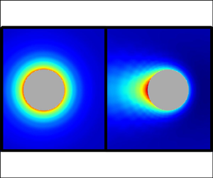
Figure 5 displays the charge  ${\textstyle \frac 12(c^+-c^-)}$, ionic strength ${\textstyle \frac 12(c^++c^-)}$ and counterion $c^-$ density configurations around the particle for $\delta =1$ at weak, moderate and strong, field regimes. Figures 5(a–c) show that the charge distribution is essentially spherically symmetric around the particle when $\beta =0.1$, characteristic of a weak perturbation to the equilibrium Debye cloud around a uniformly charged particle. The charge in this cloud is negative since $\sigma >0$. At $\beta =5$, the charge distribution has lost its spherical symmetry and displays a slight fore–aft asymmetry, and the Debye cloud appears to be closer to the particle surface when compared to the weak-field regime. At $\beta =50$, the spherical asymmetry is increased, and the electric field has stripped the Debye layer from the colloid. The fact that the Debye layer is stripped from the particle in strong electric fields explains why the electrophoretic mobility approaches the Hückel limit, since the electrokinetic retardation provoked by the Debye cloud becomes less prominent. Notably, the contribution from the electric dipole to the overall electric field, which at large distances is dominated by the imposed field, continues to be small, even after losing spherical symmetry, due to the maintained fore–aft symmetry.

Figure 5. (a–c) Charge, (d–f) ionic strength, and (g–i) counterion density distributions around the particle in (a,d,g) weak,  $\beta =0.1$, (b,e,h) moderate, $\beta =5$, and (c, f,i) strong, $\beta =50$, electric fields for $\delta =\sigma =1$ and $\alpha ^\pm =0.3$.
Figures 5(d–f) illustrate the ionic strength for the same values of  $\delta$ and $\beta$, where it can be seen that the spherical symmetry is broken when $\beta$ is not small. However, there is a different behaviour between the left and right sides of the particle. Since the particle is moving, to the right in figure 5, there are relaxation effects that become more significant at large values of $\beta$, making the ion cloud lag behind the particle as it moves. Figures 5(g–i) show the counterion distribution around the colloid. When comparing to the ionic strength, we see that the lack of ions to the right of the particle is not due to counterions. Notably, this asymmetric – in both spherical and fore–aft characteristics – counterion density distribution was proposed by O'Brien & White (Reference O'Brien and White1978), due to a disparity in the motion (relative to the particle) of the counterions at the front and at the rear of the colloid. This disparity causes the counterions to spend more time behind the particle as the latter moves. Since the colloid is only moderately charged, the coions also play an important role to reduce the fore–aft asymmetry in the charge density distribution.
Figure 6 shows the velocity field for varying values of the ion drag coefficient  $\alpha ^\pm$ and electric field strength $\beta$. Here, $\alpha ^+=\alpha ^-$, as probably best approximated by KCl. Note, however, that our numerical scheme can readily handle cases where the ionic diffusion coefficients are unequal, although this is not explored in the present work. Increasing the ion drag coefficient $\alpha ^\pm$ has a slight effect on the flow, skewing the streamlines opposite to the particle direction of motion. This would result in a retardation effect, slowing down the particle. It can also be seen that this effect is more noticeable in stronger fields, where the nonlinearity is more prevalent.

Figure 6. Streamlines of the velocity for different values of the ion drag coefficient  $\alpha ^\pm$ and electric field strength $\beta$. Here, $\delta =\sigma =1$.
The impact of  $\beta$ on the flow is more noticeable; figure 6 illustrates the transition between a flow pattern, at the particle scale, characteristic of phoretic motion to a flow pattern due to a conservative force. Namely, when $\beta =0.1$, a velocity field with a (irrotational) source dipole characteristic is visible, suggesting that the flow disturbance by the particle decays as $1/r^3$. This is the classic flow pattern for electrophoretic motion of a particle under a weak field, agreeing with the potential flow solution derived originally by Morrison (Reference Morrison1970) and Anderson (Reference Anderson1989) under the assumption of a thin Debye layer ( $\delta \ll 1$) and a moderately charged particle ( $\sigma ={O}(1)$). Schnitzer & Yariv (Reference Schnitzer and Yariv2012c) removed the weak-field restriction and showed that this potential flow solution holds for fields up to $\beta ={O}(\delta ^{-1})$. Notably, our computations suggest that the potential flow structure persists at the particle scale ( $r={O}(1)$) even beyond the small- $\delta$ limit. In the weak-field regime, $\alpha ^\pm$ has a negligible effect on the flow patterns. However, as $\beta$ increases, the effect of $\alpha ^\pm$ is evident. When $\beta =1$, the source dipole is lost to some degree, Finally, when $\beta =10$, the flow pattern resembles a sedimentation flow profile, where the flow disturbance is longer-ranged, decaying as $1/r$. This is related tightly to the ion cloud distribution shown in figure 5; as the electric field gets stronger, the Debye layer gets stripped from the colloid, reducing the magnitude of the coupling between the flow, ion transport and electric field, which leads to a conservative body force in the flow momentum equation. The important implication is that the common notion of hydrodynamic interactions between moderately charged particles undergoing electrophoresis being weak is invalidated at sufficiently strong fields. That is, at strong fields, the $1/r$ velocity decay at the particle scale would result in hydrodynamic interactions similar to particles undergoing sedimentation, for example. The present discussion has focused on the flow profile and ion distributions at the particle scale. In Appendix A, we present results for how the disturbance to the applied electric field varies at large distances from the particle. The results therein confirm that a sedimentation flow profile is attained at large $\beta$.
4.2. Highly charged particles, $\sigma \gg 1$

For the case of highly charged particles, a refinement in the computational mesh was imperative to obtain converging results. The high charge on the colloid exacerbates the presence of the boundary layer at the Debye scale, leading to numerical errors with the above-mentioned number of nodes. Convergence was reached when using  $40^2$ nodes distributed using the same radial and angular progressions after an adaptive mesh refinement. This resulted in a mesh with size $0.004$ in the particle neighbourhood. Furthermore, due to the small size of the Debye layer, visual depictions of the ion cloud, as in figure 5, are difficult to make; hence we focus on computing the electrophoretic velocity and comparing it to known results.
Figure 7 shows a comparison to the asymptotic expression from Schnitzer & Yariv (Reference Schnitzer and Yariv2014) obtained from analysis of their thin-Debye-layer macroscale model at small  $Du$ (see (1.4)) and small $\alpha ^\pm$. They refer to the latter condition as a ‘small-ion’ approximation, which means that the Péclet number is also small. The comparison is performed on the deviation from Smoluchowski's formula; that is, we compute the field-dependent mobility
 \begin{equation} \mu_1=\frac{1}{Du}\left(\frac{U}{\beta}-\zeta_0\right). \end{equation}
Here,  $\zeta _0$ is the zeta potential at weak electric fields and negligible ionic polarization, and it is related to the surface charge density by $\zeta _0=2\ln (\delta \sigma )$. The small-ion asymptotic expression from Schnitzer & Yariv (Reference Schnitzer and Yariv2014) is given by
 \begin{equation} \mu_1={-}4\ln\left(\cosh\frac{\zeta_0}{4}\right)-\zeta_0+\frac{2}{21}\,\beta^2. \end{equation}
Figure 7. Comparison of the electrophoretic mobility deviation  $\mu _1$ (see (4.4)) from Smoluchowski's formula to the small-ion asymptotic expression from Schnitzer & Yariv (Reference Schnitzer and Yariv2014) in (4.5). Here, $\delta =0.02$, $\sigma =213$, $\alpha ^\pm =0.01$, $\zeta _0=3$ and $Du=0.1$.
The first two terms in (4.5) address the inadequacy of Smoluchowski's formula in the case of highly charged particles in weak fields, while the last term represents the nonlinearity of the electrophoretic mobility in field strength. Our numerical computations and (4.5) exhibit the transition of the ion cloud from acting as a retardation effect to an enhancement, to the overall electrophoretic velocity as  $\beta$ increases. This is evidenced by the sign change of $\mu _1$ with increasing $\beta$ in figure 7. We view this agreement as a validation of our numerical computations. We stop our computations at $\beta =10$ to avoid numerical instabilities that arise at stronger fields. These instabilities can be managed by using a finer mesh, which would lead to larger computation times.
This transition from retardation to enhancement is not restricted to thin Debye layers: it also appears in the case  $\delta ={O}(1)$, as shown in figure 8(a). For low values of $\sigma$, the mobility transitions from Henry's formula to a superlinear behaviour as was shown in figure 3; and the electrophoretic mobilities for $\sigma =0.1$ and $\sigma =1$ remain close for any value of $\beta$. However, for a more highly charged particle ( $\sigma =10$ in the figure), the mobility in the weak-field regime is lower than the value predicted by Henry, then it transitions smoothly to an enhanced mobility as $\beta$ increases; this is in line with the prediction of Schnitzer & Yariv (Reference Schnitzer and Yariv2014) for thin Debye layers.

Figure 8. Scaled electrophoretic mobility  $\mu$ (see (4.1)) versus (a) $\beta$ at different values of $\sigma$, and (b) $\sigma$ at different values of $\beta$. Here, $\delta =1$ and $\alpha ^\pm =0.3$.
Figure 8(b) also displays how increasing  $\sigma$ causes a reduction in the mobility at weak-to-moderate electric field strength. However, in the strong field regime, increasing the surface charge $\sigma$ has only a slight effect on the mobility, since this is already approaching Hückel's result.
The comparisons in figures 7 and 8 were made with specific values of  $\delta$. In the comparison to Schnitzer & Yariv (Reference Schnitzer and Yariv2014) in figure 7 for $\delta =0.02$, a retardation effect of the Debye cloud (i.e. negative $\mu _1$) is still seen at $\beta ={O}(1)$. Thus in this case, a weak-field response is seen even at non-small values of $\beta$. This is not true for the case of $\delta =1$ as shown in figures 3 and 8. Therefore, the transition from retardation to enhancement is also $\delta$-dependent, as was the case of the departure from the linear electrophoretic velocity.
Figure 9 illustrates the effect of  $\alpha ^\pm$ on the nonlinear contribution to the electrophoretic velocity. The comparison is made in the nonlinear contribution to the electrophoretic speed $U_{nl}$; this is obtained by subtracting the linear speed $U_l$ from the total velocity $U$. The linear speed is calculated as $U_l=\mu _0\beta$, where $\mu _0$ is approximated as the total electrophoretic mobility at $\beta =10^{-2}$. The slope of all three curves is approximately $3$ over the range of $\beta$ examined, with a small deviation for larger values of $\beta$ and $\alpha ^\pm$. This is in good agreement with the weakly nonlinear analysis (Schnitzer et al. Reference Schnitzer, Zeyde, Yavneh and Yariv2013), since the leading behaviour of $U_{nl}$ is ${O}(\beta ^3)$. Furthermore, at fixed $\beta$, $U_{nl}$ increases with increasing $\alpha ^\pm$ (over the range of $\alpha ^\pm$ examined), in agreement with Schnitzer & Yariv (Reference Schnitzer and Yariv2014).

Figure 9. Nonlinear electrophoretic velocity  $U_{nl}$ for different values of $\alpha ^\pm$. Here, $\delta =0.02$, $\sigma =213$ and $\zeta _0=3$. The connecting dashed lines are for visual purposes only.
A comparison to experimental results from Tottori et al. (Reference Tottori, Misiunas, Keyser and Bonthuis2019) is presented in figure 10. Those authors measured the speed of polystyrene (PS) and polymethyl methacrylate (PMMA) particles immersed in a KCl solution in a microfluidic channel. The particles move due to a combination of electrophoresis and advection in an electro-osmotic flow resulting from the charged channel walls. The comparison is made in the nonlinear contribution to the electrophoretic speed; here, the linear component of the speed encompasses both linear electro-osmotic and electrophoretic components. Our numerical predictions are in good agreement with the experiments for both PMMA and PS particles. In both cases, the thin Debye layer represents a mathematical boundary layer, wherein the ionic concentrations and electric potential vary rapidly, making numerical computations challenging. Just as for the comparisons in figure 7, a refinement in the mesh was necessary to obtain converging results, especially in the case of PMMA particles. Their experiments for both particles correspond to the thin-Debye-layer limit, both particles are highly charged, and the field strength is weak to moderate. More specifically, in the case of PMMA particles,  $\delta =0.03$, $\beta _{max}=3$, $\sigma =-890$, $\alpha ^\pm =0.45$ and $\zeta _0=-6.5$; while for PS particles, $\delta =0.04$, $\beta _{max}=2.5$, $\sigma =-190$, $\alpha ^\pm =0.45$ and $\zeta _0=-4$. The values of $\delta$ and $\beta _{max}$ are approximately the same for both particles; however, PMMA particles have a significantly larger $\sigma$ than PS particles, resulting in more prominent nonlinear electrophoresis (and more challenging computations).

Figure 10. Comparison of the nonlinear electrophoretic velocity  $U_{nl}$ with experimental results from Tottori et al. (Reference Tottori, Misiunas, Keyser and Bonthuis2019). Blue: PMMA particles with $\delta =0.03$, $\beta _{max}=3$, $\sigma =-890$, $\alpha ^\pm =0.45$, $\zeta _0=-6.5$. Red: PS particles with $\delta =0.04$, $\beta _{max}=2.5$, $\sigma =-190$, $\alpha ^\pm =0.45$, $\zeta _0=-4$.
5. Conclusion
We have presented a numerical technique to compute the electrophoretic velocity of a uniformly charged, spherical, rigid, dielectric particle for, in principle, arbitrary Debye length and electric field strength. Specifically, we developed a spectral element method to solve the full nonlinear electrokinetics to this end. For moderately charged particles, we showed that the electrophoretic mobility transitions smoothly from Henry's formula to a superlinear mobility with increasing  $\beta$. Regardless of the value of $\delta$, the electrophoretic mobility tends to the Hückel limit for sufficiently large values of $\beta$. However, the rate of this transition to the Hückel limit in strong fields is $\delta$-dependent. In addition, we demonstrated how the fluid flow around the particle transitions from a phoretic-like pattern in weak fields to that induced by a conservative force when $\beta \gg 1$. In the case of highly charged particles, our results compare well with previous experiments and asymptotic expressions. We corroborated the transition of the Debye cloud from retardation to enhancement of particle motion, as predicted by Schnitzer & Yariv (Reference Schnitzer and Yariv2014), and we showed that this behaviour is not exclusive to thin Debye layers.
Future work naturally follows, as the numerical technique can be modified to capture the transient behaviour of the electrophoretic velocity, which is of paramount importance when the particle is under the influence of alternating fields, for example. The present numerical scheme can also be expanded to take into account electrothermal effects in the electrokinetic equations, which could become prominent at large values of  $\beta$, by incorporating an energy equation, to determine the evolution of the temperature distribution around the particle. Finally, other electrostatic conditions at the particle surface would be of interest, beyond the fixed-charge assumption adopted here. For example, a natural extension would be to consider particles with surface charge regulation.
Funding
This work was supported by the National Science Foundation through grant no. CBET 2002120.
Declaration of interests
The authors report no conflict of interest.
Appendix A. Convergence test and electric field far from the particle
Figure 11 shows a convergence test to determine the number of nodes and the size of the domain. A thin Debye layer ( $\delta =0.1$) was used as a test case to determine the number of nodes, and a thick Debye layer ( $\delta =10$) was used to determine the size of the domain $R_o$. These test cases were chosen as they represent the worst-case scenarios for each of these two parameters. Figure 11(a) illustrates the exponential convergence with increasing number of nodes for different values of $\beta$. While varying the number of elements (figure 11b), the domain size was fixed at $R_o=100$, and when varying the domain size (figure 11c), the number of nodes was $20^2$. Figure 11 illustrates that the improvement, of choosing a finer mesh or a larger domain than the chosen values, is negligible in the case of moderately charged particles.

Figure 11. Convergence test of the electrophoretic mobility at weak-to-moderate fields with different numbers of nodes and values of  $R_o$. Here, $\sigma =1$ and $\alpha ^\pm =0.4$.
Figure 12 displays contours of the negative of the charge density for  $\delta =\sigma =1$ and $\alpha ^\pm =0.3$, for $\beta =0.1$, $1$,
$1$,  $10$ and $50$. The same value of charge density $c^+-c^-=10^{-2}$ is chosen in each case. At weak fields ( $\beta =0.1$ in the figure), the charge density is essentially isotropic. However, as $\beta$ increases, the contour extends in the field direction. Hence for large $\beta$, it is critical to choose the domain size $R_o$ to be sufficiently large to capture the field-driven extension of the charge cloud. For these computations, $R_o=100$. With reference to figure 11(c), this value of $R_o$ results in a calculation of the mobility that does not change appreciably if $R_o$ is increased further.

Figure 12. Contour plot of charge density distribution for  $\delta =\sigma =1$ and $\alpha ^\pm =0.3$, (a) close to the particle, and (b) far from the particle. Contours levels correspond to $c^+-c^-=10^{-2}$. Since the particle is positively charged, this corresponds to the negative of the charge density in the electrolyte.
It is also of interest to determine how the disturbance to the uniform applied field varies at large distances from the particle. Following Fixman & Jagannathan (Reference Fixman and Jagannathan1983), the electric potential can be written as the multipole expansion
 \begin{equation} \varphi={-}\beta z+\frac{1}{8{\rm \pi}\delta^2r}\left[q+\frac{1}{r^2}\,\boldsymbol{p}\boldsymbol{\cdot}\boldsymbol{r}+{O}(r^{{-}2})\right], \end{equation}
where  $q$ is the apparent charge (or monopole strength), and $\boldsymbol {p}$ is the charge dipole. Note that $\boldsymbol {p}=p\hat {\boldsymbol {z}}$ due to axisymmetry, where $p$ is the dipole strength. We can calculate these quantities from our numerical scheme as the volume integrals
 \begin{equation} q=8{\rm \pi}\delta^2\sigma+\int(c^+-c^-)\,{\rm d}V \quad\text{and}\quad\boldsymbol{p}=\int(c^+-c^-)\boldsymbol{r}\,{\rm d}V, \end{equation}
where the first term in the monopole strength is the contribution from the charge on the particle surface.
Figures 13(a) and 13(b) show the monopole and dipole strengths, respectively, for  $\delta =\sigma =1$ and $\alpha ^\pm =0.4$ over the range $\beta =10^{-2}$ to $\beta =10^2$. Interestingly, the monopole contribution is generally non-zero, although it is small for weak fields. This is in agreement with numerics from Fixman & Jagannathan (Reference Fixman and Jagannathan1983). We compute a change in sign of the monopole strength with increasing $\beta$, which was also reported in their paper (see their figure 1), although their computations were restricted to values of $\beta$ smaller than ours. The existence of a monopole contribution to the disturbance field implies that a net electric force $F_e$ is exerted on a spherical surface at large distances from the particle. In figure 13(c), we compute this electric force (i.e. the surface integral of the traction arising from the Maxwell stress) over the surface $R_o=100$. The electric force is small at weak fields but certainly not negligible at moderate and large $\beta$. Schnitzer & Yariv (Reference Schnitzer and Yariv2014) noted that a net electric force can exist on a surface enclosing the Debye layer and particle for thin Debye layers beyond the weak field limit. Since the system must be force-free (see (2.9)), a non-zero electric force over $R_o$ must be compensated by a non-zero hydrodynamic force. Thus at large distances we expect the velocity field to decay as a Stokeslet; figure 13(d) shows the streamlines around the particle, which displays the familiar pattern associated with a particle under a net hydrodynamic force. The dipole strength (which is negative) decreases initially with increasing $\beta$, again in a manner that is similar to that found in Fixman & Jagannathan (Reference Fixman and Jagannathan1983). We find a minimum in the dipole strength at $\beta \approx 10$, which is beyond the field strength that they examined.

Figure 13. (a) Monopole strength  $q$, (b) dipole strength $p$, and (c) electric force $F_e$, evaluated using a far-field radius $r=100$. (d) Velocity streamlines for the case $\beta =50$. Here, $\delta =\sigma =1$ and $\alpha ^\pm =0.4$.


