


1. Introduction
The structure of the subglacial meltwater drainage system determines the efficiency with which water is discharged from beneath a glacier, thereby determining the distribution in space and time of basal water pressure and strongly influencing effective pressure and friction. A theory of drainage is vital for the solution of one of the central unresolved problems of glaciology: that although we can empirically deduce a basal friction law for a glacier of known form, we cannot predict dynamic behaviour from a description of the bed and the climate drive without a theory of basal hydraulics.
The drainage of meltwater over rock beds has been extensively studied (e.g. Reference Röthlisberger, Lang, Gurnell and ClarkRöthlisberger and Lang, 1987) and there have been theoretical studies of drainage over till beds (e.g. Reference Walder and FowlerWalder and Fowler, 1994). In the first case the rock bed, and in the second the substratum of the till, are implicitly assumed to have very low transmissivity or to be impermeable, such that there must be longitudinal drainage over the surface of the bed and/or within the till. This is assumed to be either by flow in tunnels or in anastomosing tunnel systems which enlarge and contract as meltwater recharge varies, either diurnally, seasonally or episodically, and which result in correlative fluctuations in water pressure, effective pressure and friction (Reference KambKamb, 1987).
In fact, most rock beds have a relatively high permeability. Even where the rock matrix on a small scale is impermeable, rocks have larger-scale fracture patterns; even ancient shield rocks have, in the topmost 100m or so, hydraulic conductivities of the order of 10–6ms–1 (e.g. Gustafsson and others, 1989; Reference Rhén, Gustafson, Stanfors and WikbergRhén and others, 1997), compared with conductivities in overlying tills that can be an order of magnitude less. Not only is the permeability of bedrock often enough to have a significant impact on drainage where the water flux is derived from basal melting alone, but when it is greater than that of the overlying till, it will act as a sink for water in the till, creating a strong downward potential gradient in the till (Reference Boulton and DobbieBoulton and Dobbie, 1993).
However, it is when the glacier is underlain by thick, sometimes highly permeable, beds that groundwater flow is particularly important. Thick masses of glaciofluvial sediment of high transmissivity are likely to be common beneath modern glaciers, and were ubiquitous beneath Pleistocene ice sheets (e.g. Reference Poole and WhitemanPoole and Whiteman, 1961; Reference Eissmann, Litt, Wansa, Ehlers, Kozarski and GibbardEissmann and others, 1995; Reference SchirmerSchirmer, 1995).
Unlithified sediment beds are intrinsically more susceptible to deformation than rock beds, either by shear immediately beneath the glacier sole or by consolidation of the sediment mass by the ice load. In both cases, the structure and efficiency of the drainage system is important in determining the rate at which the sediment can consolidate in response to a change in glacier loading or meltwater recharge rate, and in determining whether shear deformation of the sediments can occur.
Notwithstanding the importance of monitoring spatial and temporal variations of the subglacial hydraulic system and the associated deformation, the difficulties of doing so are considerable. A rare opportunity to undertake such an experiment was offered in 1988. In late 1987, a compressional wave was observed on the glacier surface near the eastern margin of Breiðamerkurjokull, southeast Iceland. It was moving towards the glacier terminus in an area known to be underlain by a thick (50–80 m) sedimentary sequence overlying bedrock. In anticipation of a readvance when the wave came near to the glacier margin, the unlithified sediment bed over which the glacier was expected to flow was instrumented in an attempt to monitor the behaviour of the groundwater system without the difficulties associated with drilling from the glacier surface (unknown bed stratigraphy and structure, difficulties of drilling into the bed, disturbing the bed in indeterminate ways, maintaining monitoring cables through the zone of basal décollement).
Monitoring was largely successful, and this paper describes the results of this natural experiment, presenting a theoretical analysis of the drainage and consolidation process and identifying important implications. The controlled natural experiment revealed the transient behaviour of a composite ice-till-aquifer system at the full spatial scale and almost full temporal scale of the event. Nothing of this type can be revealed by laboratory experiments. They lack the spatial scale captured by the field experiment, of 50cm between transducers, 20–30m between test sites and of the 1000m scale of the groundwater reservoir reflected by aquifer measurements; moreover, the characteristic scale in laboratory experiments is small (<10cm), and water flow is of negligible power, and cannot address issues of ice-till-aquifer coupling. Unfortunately, the 6 hour interval between field measurements was just too large to capture the full pressure response to diurnal melt cycles. This was, however, observed in a later experiment with higher-frequency monitoring (Reference Boulton, Dongelmans, Punkari and BroadgateBoulton and others, 2001b), permitting the full spectrum to be captured, from advance over the site and establishment of quasi-equilibrium to short-period diurnal oscillation.
2. Sedimentary Setting
Figure 1 shows the terminus area of the glacier Breiðamerkurjökull. Figure 2 shows the nature of the surface beyond the margin of the glacier before the local mini-surge, and the areal extent of the mini-surge east of proglacial lake Jökulsárlón. The surface is moulded into a series of drumlins and bears long, flow-parallel flutes on its surface. The proglacial surface has been progressively deglaciated during the 20th century (e.g. Reference Evans and TwiggEvans and Twigg, 2000, 2002), interrupted by brief phases of readvance, and short winter readvances that generate winter push moraines (Reference BoultonBoulton, 1986) which reflect the form of the retreating glacier margin. They demonstrate that lobate extensions of the glacier margin, associated with narrow zones of faster flow, occurred in the troughs between drumlins.

Fig. 1. Map of the terminal and proglacial zones of Breiðamerkurjokull, southeast Iceland, in early 1989. The outermost moraines (lower bold line) were formed at the maximum Little Ice Age advance between 1895 and 1905. The subsequent retreat of about 5 km has exposed a series of large lakes and, on land, areas of till (marked by lined shading) and intervening areas of glaciofluvial outwash. The lines on the till surface show the orientation of flow-parallel drumlins and flutes and the locations of major transverse moraines that mark halt or readvance of the glacier margin during overall retreat. The 1989 glacier margin is shown (upper bold line), together with the fast ice stream that flows into proglacial lake Jokulsarlon. Medial moraines are the other shaded areas on the glacier surface. The line A-B indicates the section from 0 to 2000m shown in Figure 3.

Fig. 2. The area to the northeast of proglacial lake Jokulsarlon showing the 1988 readvance and the location of the transect (the continuation of B-A in Fig. 1) along which the monitoring described in this paper was undertaken. The area marked L is the lake shown in Figure 5. The scale is in metres.
The proglacial surface that was later overridden by the mini-surge had an almost complete cover of till which was up to 2m thick (exceptionally up to 4m in push moraines), underlain by sands and gravels that appear to represent the top of a thick stratum of outwash sediments. These were proven by a 31m deep borehole drilled in the position shown in Figure 3 after the mini-surge had ended and retreat had recommenced. A seismic survey (Reference Bogadóttir, Boulton, Tömasson, Thors and SigbjarnarsonBogadóttir and others, 1986) suggested thicknesses of up to 90–130m of sediment above bedrock in the vicinity of the site, with a significant change in sediment properties in the lower part of the sequence (Fig. 3). Experience elsewhere on Breiðamerkursandur and interpretation of the origin of the sandur (Reference Boulton, Harris and JarvisBoulton and others, 1983) suggest that the latter might be finegrained sediments. A radio-echo survey was undertaken after the mini-surge to determine the form of the ice-bed interface. This linked with the later more extensive survey of Bjornsson (1996), and showed that the ice-bed interface dips systematically to the north, forming a major subglacial scarp. It has been suggested (Reference Boulton, Menzies and RoseBoulton, 1987) that other, similar scarps on Breiðamerkursandur represent former locations of large ice-contact outwash accumulations. We have projected the apparent sediment bedrock interface in the proglacial zone beneath the glacier in Figure 3.

Fig. 3. Section through the terminal zone of Breiðamerkurjökull along the line A–B shown in Figure 1, measured during summer 1989. The line of section is collinear with the transect in Figures 5 and 7 and has the same reference point for horizontal and vertical coordinates. The glacier bed is reconstructed from a radio-echo survey which went as far as 1200m from the reference point, where heavy crevassing prevented further progress. The bed profile between 1200 and 1900m was reconstructed from Reference BjörnssonBjörnsson’s (1996) more extensive survey. The apparent scarp between 1200 and 1300m may be a product of a mismatch between the two surveys, although it is possible that the scarp is real and may coincide with the sub-crop of possible muddy sediments and underlying basaltic bedrock. The sediment stratigraphy beyond the glacier margin is inferred from a seismic survey (Reference Bogadóttir, Boulton, Tömasson, Thors and SigbjarnarsonBogadóttir and others, 1986) and from the borehole marked on the section. Subglacial sediment stratigraphy is extrapolated from the proglacial evidence.
The topmost parts of the sedimentary sequence lying above bedrock and beneath the surface till are exposed in natural sections up to 10 m deep (Fig. 4). They are highly variable sands and gravels, ranging from poorly sorted, silty, sandy gravels to pods of highly porous, clast-supported gravels. There is evidence of washing down of significant quantities of silt from the till into the upper part of the sands and gravels (e.g. Reference Boulton and DentBoulton and Dent, 1974). In some places there is an internal non-sequence where younger gravels lie upon the eroded surface of older gravels, with, sporadically, an in situ moss peat horizon at the interface. We interpret the peat-covered surface as the stable, vegetated surface of Breiôamerkursandur as it was immediately before the glacier overrode the area in the 1740s (Reference Boulton, Harris and JarvisBoulton and others, 1983) and which was part of the fields of the historical farm Breiðá. We interpret the underlying, older, gravels as outwash of an earlier period, the overlying gravels as outwash laid down by glacial rivers in front of the advancing glacier in the 18th century, and the till as a product of the Little Ice Age advance before the glacier retreated from its maximum extent at the beginning of the 20th century. We have no evidence for the existence of older tills within the outwash sequence. The drilling method did not recover cores, and bulk samples from drilling are likely to have had any fine materials representing till matrix washed out during sampling. Given the thin nature of tills on Breiðamerkursandur, and evidence in sections across the sandur plain of thick, coarse, subsurface outwash strata, we believe that most of the sediment represented in the section above –60 to –70m in Figure 3 is coarse glaciofluvial outwash. This varies from silty-sandy, matrix-supported gravels, to clast-supported gravels, to diamictons typical of proximal alluvial fan environments, to poorly sorted sands and potentially to lacustrine and marine silts and clays dating from the early Holocene infilling of a previous fjord (Reference Boulton, Harris and JarvisBoulton and others, 1983). This variability is consistent with evidence from pumping tests in the borehole shown in Figure 3 (and at other sites). A slotted casing and packer system was used to conduct pumping tests at specific horizons. These yielded ranges of hydraulic conductivity from 2.2 × 10⁻³ to 7.4 × 10⁻⁷ m s–1, which reflects the wide range of lithologies observed in the fluviatile sequence and may even reflect sampling of tills, or lacustrine or marine clays that were not found exposed at the surface. A pumping test using the full length of the unpacked casing, a probable reflection of overall conductivity, yielded values of the order of 10–6ms–1. This suggests that the aquifer is compartmented and that low-conductivity horizons exercise an important control on overall conductivity. Such a compartmentalized structure would be consistent with the lenticular form of outwash-fan sediment bodies.

Fig. 4. Schematic composite section of the uppermost 10m of the stratigraphy in the immediate vicinity of the mini-surge area. The moss peat horizon probably represents pasture of the historical farm Breiðá, destroyed by outwash rivers in the 1740s (personal communication from F. Bjornsson, 1976), prior to the advance of the glacier to its Little Ice Age maximum extent (Fig. 1).
3. Glacier Flow and the Mini-Surge
An overdeepened trench extends through proglacial lake Jökulsárlón and far beneath the glacier (Reference BjörnssonBjörnsson, 1996). This trench is up to 150–250m deep, 1–3 km wide and is dammed by the Little Ice Age terminal moraines of the glacier to the south and the glacier ice cliff to the north (Fig. 1). This overdeepened axis is also an axis of a relatively fast-flowing glacier stream. Observations over a 30 year period show that, from time to time, there is a strong ice pulse along this axis, which projects a compressional wave through the ice to the east of the stream, leading eventually to a small surge of the glacier margin to the east of Jökulsárlón. An eastward shift of the stream in 1986–88 generated such a compressional wave. During this period, there was a transient flow divide in the glacier ~1 km to the north of the experimental site (Fig. 1), separating a zone to the north of strong glacier flow towards Jökulsárlón, from ice flowing towards the margin to the east of Jökulsárlón.
Figure 5a shows the form of the glacier margin and the proglacial area during the early part of the mini-surge, and the location of the outer part of the transect from which results are reported in this paper. The terminal slope of the glacier is smooth and little crevassed, although it contained numerous narrow fractures, some of which were closed, but others permitted drainage of surface water. However, a prominent compressional wave can be seen ≈250m from the glacier terminus. Behind it, the glacier surface is heavily fractured by predominantly longitudinal crevasses reflecting strong longitudinal compression and transverse extension. The movement of the glacier front along the transect from 130 to 0m, and the profile of the glacier surface in the marginal zone was surveyed by laser distance finder from points in the proglacial area on a frequent, although irregular, basis (Fig. 6). By early March 1988, the glacier margin had begun to advance, at an average rate of ~1md–1, and had reached its maximum extent by mid-September (approximately day 200). It remained at its maximum extent until about day 210, and then began to retreat at an average rate of ~0.2m d–1 until at least day 230.

Fig. 5. The glacier terminus during the mini-surge. (a) The glacier terminus and proglacial zone in the area of Figure 2 in early June 1988, when the glacier had reached about 55m from the transect (see Fig. 6). The line of the instrumented trench (see Figs 6 and 8) is shown by the dashed line. The 0m reference point is marked X, and lies on a clearly defined push-moraine crest that marks the extent of a small readvance in 1982 (see Figs 2 and 7). The steep face of the wave on the glacier surface can be clearly seen, together with the smooth, uncrevassed ice in front and the highly crevassed ice behind. The lake in the foreground is that shown in Figure 2. (b) The glacier terminus and proglacial zone in late November 1988, during the very early stage of retreat of the glacier from the late October maximum advance. The twin-crested moraine shown between 0 and –10m in Figure 7 can be clearly seen. The outer crest is the 1982 push moraine and the inner crest that of the 1988 mini-surge push moraine. The lake in the foreground is that shown in (a)). The data logger was sited at the base of the promontory marked D (also visible on the right shore of the lake in (a). The poor quality of the image reflects a higher-altitude photograph and difficult flying conditions.

Fig. 6. Measured glacier profiles along the transect shown In Figure 7 during the mini-surge. The evolving cross-sectional form of the push moraine at the glacier front is shown by dashed lines. The final push moraine at 0m was emplaced by the surge. The timing of each profile is given by the number of days after the start of the experiment on 1 March 1988, with the date (day.month) in parentheses.
4. Experimental Set-Up
Prior to the advance shown in Figure 6, a motorized mechanical digger was used to dig a number of trenches both parallel and transverse to the direction of advance of the glacier in a zone up to 135m behind the eventual maximum extension of the glacier. Where the till base was relatively shallow (generally <2 m), and where large (>0.5m diameter) till boulders did not inhibit digging, trenches were dug to below the base of the till, which was seen to lie on sands and gravels.
Figure 7 shows the stratigraphy of a longitudinal trench (see Figs 2 and 5a for location) that was chosen for particularly thorough instrumentation because it had a thicker till than the other trenches and many other proglacial areas at Breiðamerkurjökull, where the till is rarely greater than 1m thick. Samples of till granulometry are shown in Figure 8. The till was relatively coarse-grained in the outer part of the transect and relatively fine-grained in the inner part, particularly in its lower part. The sands and gravels were similar to those reported above from natural sections, and appeared to all belong to the latest phase of sub-till outwash activity (Fig. 4).

Fig. 7. The profile of the experimental transect at Breiôamerkurjökull shown in Figures 2 and 6 and the stratigraphy observed in the trench before the mini-surge. The locations of water-pressure transducers are shown by crosses. The instrument cable was laid along the trench floor and connected to the data logger shown near the lake shore. The mini-surge produced a new moraine to the right of that shown in the figure (see Fig. 6).

Fig. 8. The grain-size distribution of till sampled in the trench (Fig. 7). An upper and a lower till sample were analyzed from each transducer site prior to the experiment (marked 12U (transducer T12 in Fig. 7, upper sample), 12L, 30U, 30L, etc.). The phi scale is used, where 100 is 1 mm, 00 is 1mm and –60ϕ is 64 mm. The percentages are those contained in the phi interval above that of the given unit. Rare clasts of the order of metres in size exist in the till. The inner part of the till tends to be finer-grained than the outer part. The 125 and 85m samples from the inner transect are shown with bold lines.
Whilst the trench was open, pore-pressure transducers were inserted into the till and the underlying gravels at locations shown in Figure 7. The electronic transducers were of series 4-308 made by Gems Sensors Limited, with a range up to 350 kPa, an accuracy of approximately 1% at temperatures between 0 and 8°C, a response time of milliseconds and long-term drift of 1–2% a–1. They were of diaphragm type, with the diaphragm protected by a high-permeability plate and the transducer mounted in a 31.8mm diameter, 178mm long housing. They were connected via steel-mesh sheathed cables laid along the base of the trench to a transmitter and a digitally recording data logger with an accuracy of better than 0.5%, located as shown in Figure 7. Till and underlying glaciofluvial gravels were carefully segregated from each other during trench construction. The trench was refilled, first with glaciofluvial sediment, which was compressed until its surface was approximately level with the top of the in situ sediment, and then with till, consolidated so that it was level with the surface. Unfortunately, the data logger had to be left unattended for long periods and had limited battery life, so measurements of pore pressure were only taken every 6 hours. As a consequence, higher-frequency patterns of pore-pressure fluctuation were not recorded except in shortterm tests at the end of the experimental period, by which time most till transducers had ceased recording.
A number of magnets were inserted into the till in the walls of the trench. Some were recovered subsequently, and indicated those levels in the till that had remained stable and those that had moved by deformation of the till.
5. Geological Consequences of the Mini-Surge along the Transect
No water table was found during digging of the trench. We presume that this reflects its relatively elevated position and the thick underlying aquifer, able to drain infiltrating water readily, both into the small lake to the south of the transect and towards the glacier margin. During the whole of the advance, however, in a zone extending for 15–30m beyond the glacier margin, the till was saturated to the surface. This demonstrates that the advance of the glacier strongly increased recharge into the upper part of the aquifer and the till, thereby driving up the water table. Enhanced flow from the stream draining the small lake to the south of the transect (Figs 5 and 7) probably reflected enhanced groundwater flow into the lake, driven by the advancing glacier’s impact on groundwater pressures.
The advance of the glacier front created a push moraine. This was composed of till which our observations suggest was created by ‘ploughing’ of the glacier margin into the pre-existing till rather than till being extruded from beneath the glacier. The push moraine grew in size as the glacier advanced from 120 to 55m along the transect, but then diminished (Fig. 6), suggesting that the glacier began to override the moraine as its mass offered increasing resistance to glacier movement.
The till surface observed after glacier retreat from the experimental area was fluted. Photographs taken before and after the surge showed that a new set of flutes had been created on the till surface, replacing the flutes on the presurge surface. Moreover, the fluted surface showed no sign of water erosion, demonstrating that there had not been strong meltwater drainage across its surface. Nor were there any signs of major canalized drainage in the immediate vicinity of the transect, apart from small-scale runnels and sorted sediment ridges that probably marked the location of open crevasses at the end of the surge period. We suggest that any major channels drained towards Jökulsárlón, either transversely to the east of the ice-flow divide, or along the line of the ice stream to the northwest of the divide (Fig. 1).
6. Monitoring the Surge and Water-Pressure Fluctuations
It is suggested that the enhanced groundwater fluxes that were inferred from surface upwelling or water-pressure monitoring were largely derived from surface precipitation that penetrated to the bed through crevasses and fractures (cf. Reference Fountain, Jacobel, Schlichting and JanssonFountain and others, 2005), with a minor contribution from basal melting. We initially assume all groundwater was derived entirely from the glacier section that extends from the local ice divide to the terminus as described in section 3 (Fig. 1).
The flux of surface-derived water was estimated as follows: An automatic weather station was set up to measure cumulative precipitation over 6 hour periods. Ablation rates were measured on a daily basis from 1 March 1988 (day 1 of the experiment) until 17 April (day 48), then on five separate days until 10 May (day 71), then continuously until 17 July (day 138), then on 11 separate days until 31 October (day 245). Measurements were taken of a series of 23 ablation stakes, protruding about 1m above the ice surface, set within an area of approximately 100m parallel to flow and 50m transverse to flow. They were emplaced, wherever possible, where the surface was parallel to the average slope of the measured area, and not on seracs or within the depressions surrounding individual moulins and crevasses. Stakes were reset every 7–10 days during periods of continual measurements, and during the previous evening for single-day measurements. An energy-balance model based on that of Reference Braithwaite and OlesenBraithwaite and Olesen (1989) was used to compute the theoretical ablation rate from radiation, vapour pressure and temperature data recorded by the weather station. A correlation between the theoretical and observed rate for the days on which melting was measured was used to interpolate runoff for the days on which ablation was not measured. Values of surface water production determined by this approach are shown in Figure 9. Six-hourly estimates were made for part of the period using the energy-balance model and precipitation measurements. The basal meltwater flux was estimated from the geothermal flux (Reference Flovenz and SaemundssonFlovenz and Saemundsson, 1993) and from calculated frictional heating as one to two orders of magnitude less than the surface-derived flux and is therefore assumed to make an insignificant contribution to the subglacial flux.

Fig. 9. Estimated average rates of glacier surface water production per unit area (melting + precipitation) in a zone extending, on average, 100m from the glacier terminus and 50m in width.
The glacier surface in front of the advancing compressional wave (Fig. 5a) had few crevasses but numerous small fractures, dominantly oriented parallel to and within 30° of the direction of glacier movement, presumably reflecting a state of longitudinal compressive stress. However, the glacier surface was highly crevassed behind the wave.
Figure 10 shows the record of pore pressures during the 242 day measurement period, from 1 March to 28 October, at transducers installed at 12, 30, 65, 85 and 125m along the transect, and Figure 11 shows some details of the records. Of the 14 transducers that were emplaced, 11 recorded for some or all of the experimental period. Problems occurred at the 12m site. One till transducer recorded no data, another recorded but the data have been difficult to interpret, and the transducer in the aquifer showed a 6 hour oscillation that we have not been able fully to explain and which we believe to be an artefact. However, this transducer showed an overall trend similar to the other transducers, which we therefore take to be representative of the trend of aquifer pressures at this site. Figure 10 also shows the ice pressure at each site, calculated from the surveyed form of the glacier during the surge. The transducers in the gravel aquifers at 12, 30 and 65m recorded until the end of the experiment, as did transducers in the till at 30 and 12 m. None of the till transducers at the 125, 85 and 65m sites continued recording until the end of the experiment. For example, at 65 m, the uppermost transducer, at a depth of 0.6m in the till, ceased recording after 121 days and the transducer at 1.25m in the till, ceased after 134 days. The transducer in the gravels continued recording until the end of the experiment. We suspect that transducer failures reflect breakage or pinching of the transducer leads as a result of deformation of the bouldery till. The 0.6m transducer at 65m was located at the end of the experiment, and found to have moved horizontally by several metres.

Fig. 10. Records of water-pressure transducers and estimates of ice pressure at the sites shown in Figure 7. Cessation of transducer records is assumed to reflect initiation of deformation in the sediment around them. (a) Data from the 125 and 85m sites. (b) Data from the 65, 30 and 12m sites. The inset in (a) shows a detail from the lower 85m and upper 125m transducers, compared with the average water production rate.
The general patterns of pressure variation shown in Figure 10 indicate a fairly well-defined pattern of drainage through the sediments. In any vertical sequence, the upper transducers tend to show the highest average water pressures (see also Fig. 11b). At the 65 and 85 m sites, the average water-pressure gradient between the upper transducer in the till and the top of the gravel is between ~5 and 20 kPa m–1, whilst the apparent horizontal pressure gradient is much less, about 2–3 kPa m–1, suggesting that flow through the till is dominantly vertical. A pair of transducers located at 82m (not shown here) reflect this. The horizontal water-pressure gradient in the gravel is approximately the same as in the till, but the much greater conductivity of the gravel compared with the till (one to four orders of magnitude) reflects the dominant role of the gravel in discharging the meltwater flux horizontally (cf. Reference Boulton and DobbieBoulton and Dobbie, 1993).

Fig. 11. Some details of transducer records for specific hydraulic events and anomalies (as in Fig. 10, light blue indicates the lower till transducer, dark blue the upper till transducer and red the aquifer transducer). (a) Pressure patterns in the marginal zone of upward groundwater flow at the 65m site. (b) Normal diurnal pattern of transducer pressures associated with downward groundwater flow through the till at the 65m site. (c) Transient phases of upward flow in the till during periods of relatively strong water-pressure fluctuations in the aquifer at the 65m site. (d) Convergence of aquifer and till pressures after a strong till pressure peak at the 85m site. Note that the 6 hour sampling frequency limits the precision with which peaks and troughs can be resolved, and almost certainly hides lags in the phase response to variations in pressure on the till surface (contrast with Fig. 17).
The predominantly vertical pressure gradient in the till must predominantly reflect diffuse sources of recharge of water from the glacier rather than from highly localized crevasses. The analysis that follows (sections 7, 8 and 10), shows that the typical penetration time of water from the glacier surface to the bed is less than 6 hours. Samples of ice from below the level of strong surface melting do not support the view that intergranular flow could be the dominant pathway for surface water to the bed, and crevasses are too sparse to be diffuse water sources. We think it most likely that the relatively closely spaced fractures in the ice are the dominant water-flow pathways, as demonstrated for Storgläciaren, Sweden, by Reference Fountain, Jacobel, Schlichting and JanssonFountain and others (2005). They measured flow speeds in such fractures as 0.5–4cm s–1, which is consistent with the penetration times inferred at Breiðamerkurjökull. It is noticeable, however, that water overpressures occur at the 125, 85 and 65m sites (Fig. 10) during the most rapid phase of advance and as the steepest part of the glacier front approached the sites. We assume that this must have occurred as a consequence of englacial pathways, which could have been moulins or fractures that were dipping down-ice and that were pressurized as a consequence of greater ice thickness.
Maps of the locations of crevasses and moulins that had the potential to drain surface waters were produced several times during the mini-surge, in an attempt to estimate some of the major locations through which surface water is recharged to the bed. Longitudinal crevasses were frequent in the lee of the surface wave with typical transverse spacings of 5–10m (Fig. 5a). One specific crevasse, ~8m in length, that drained a particularly large area of the surface was located close to the 125m transducer at about day 100. This coincides with a period during which the water pressures at this site showed an anomalously large response to a surface water recharge peak during the period 98–103 days, compared with the response of other transducers. It is suggested that the crevasse provided a route for a particularly concentrated drainage flux to the bed. The same crevasse was close to the 85m transducer at about day 140, when this transducer also showed an anomalously large response to a recharge peak during days 135–142 (Fig. 10a). We presume this reflects enhanced local recharge to the bed via a crevasse that had a particularly large surface catchment area.
Immediately beyond the terminus of the glacier, water pressures tend to be very close to the ice overburden pressure, reflecting the escape of groundwater from beneath the glacier (see also Fig. 11a). Subsequently, during the early stage of advance over each site, water pressures increase very rapidly, with the occasional development of excess water pressures. This appears to occur where the rate of advance of the glacier terminus is greatest (see also Fig. 11a).
The advance culminated after about 150 days, after which the remaining operational transducers at 65, 30 and 12m show a general decline in water pressures that is not associated with a decline in surface meltwater production rate. We have no direct evidence that permits us to explain this, but suspect that it may reflect the development of subglacial streams draining laterally towards Jökulsárlón.
7. A Model of the Operation of the Subglacial Hydraulic System
7.1. Approach
Before attempting a fuller explanation of the data, we develop a theory of the operation of the hydraulic system in which the flux of meltwater and sediment transmissivity determine the water pressure in the sediments for a given ice load. There are strong diurnal variations in surface meltwater production, which are transmitted through the glacier and till into the aquifer and produce variations in water pressure and sediment effective pressure. These variations in basal water pressure and the average water-pressure profile depend on the rheology of the subglacial sediments under the varying ice load caused by the advance and subsequent retreat of the glacier. Although it is clear that the tills at the site underwent shear deformation during the mini-surge, we believe that our experimental data only record pressures in the sediments beneath the deforming horizon, because of the fall in water pressure that occurs immediately before transducers cease recording, which we interpret as reflecting the beginning of sediment dilation produced by shear deformation. We therefore ignore shear deformation in the theory and modelling presented below.
We use poroelasticity theory to account for the spatial and time-dependent distribution of basal water pressure during the period of rapid ice loading as the glacier advances. The objective is to use as many of the available field data as possible as input to a model and to restrict the intrinsic model parameters to the minimum possible number, producing a model capable of predicting water-pressure profiles in the till and aquifer in response to an arbitrary time-varying recharge in which consolidation of the subglacial till layer is taken into account. Physical parameters were restricted to the permeability and volume compressibility of subglacial sediments (responsible for the compaction/dilation of porous material) and an additional parameter related to the glacier’s ability to deliver water from the ice surface to the subglacial till. This latter was introduced for the general case, but proved to be redundant for our experimental site because of the rapid transmission of surface water to the bed.
The irregularity of surface elevation, till thickness, till permeability and, most importantly, the evolving upper boundary condition of a spatially distributed ice load moving upslope, rendered a finite-difference or finite-element approach inappropriate. The chaotic nature of the surface water production data (Fig. 9), containing frequency components from 6 hours to almost half a year, presents a further complication. To deal with these complexities we have developed a mathematical model similar in operation to an analogue computer, where the entire area of interest is represented by a one-dimensional array of interconnected vertical cells (Fig. 12). Each cell represents a hydraulically interconnected thin vertical slice of ice, till and aquifer. The advantage of this approach is that the hydrodynamics of water in the cell can be analytically resolved for a given water production rate at the ice surface (at the top of the cell) with the incoming and outgoing water flux to the left and right of the cell accounting for the horizontal water dynamics. The total water-pressure field can be computed for given Fourier components of the runoff data and ice load through the numerical solution of a complex matrix equation using a standard Fortran library subroutine. The final result is given as a sum of the inverse Fourier components. The model was tested against analytic solutions for some simple approximations and produced extremely accurate results for spatial resolution, even for a relatively small number of vertical cell elements. The results are consistent with the assumption that subglacial groundwater flow lies in a flow-parallel vertical plane, apart from at the end of the experiment, when we suggest that local transverse channels developed some distance back from the maximum extent of the advance.

Fig. 12. The cell model used for hydraulic analysis. The assumed longitudinal flow system is represented by a one-dimensional array of cells representing ice (i superscript), till (t) and aquifer (a). ![]() and Pa are water-pressure potentials at the base of the glacier, in the middle of the till and at the top of the aquifer, respectively, with a varying thickness,
and Pa are water-pressure potentials at the base of the glacier, in the middle of the till and at the top of the aquifer, respectively, with a varying thickness, ![]() , of each column. The water exchange between different cells is assumed to take place in the aquifer only. Apart from the first and last, cells have a horizontal extent of 1m along the transect.
, of each column. The water exchange between different cells is assumed to take place in the aquifer only. Apart from the first and last, cells have a horizontal extent of 1m along the transect.
7.2. Water flow in consolidating subglacial sediments
7.2.1. Introduction
In the theory of consolidation, soils react differently to the same effective stress increment depending on their deformation history. Figure 13 shows a typical stress/strain relationship for a soil under uniaxial loading. The virgin consolidation curve, representing the initial compression of the soil during sedimentation and subsequent loading, shows a steady irreversible consolidation along the plastic yield envelope (OAB), along a ‘normal consolidation line’ (NCL) with a fairly high coefficient of compressibility. If the soil is unloaded then reloaded, it follows an expansion (swelling)–recompression loop (BCD). In this region it is ‘overconsolidated’. A soil can store its history of prior, higher consolidation (‘pre-consolidation’), with a lower void ratio than it would have had it undergone virgin consolidation up to its current load. Reference Boulton and DobbieBoulton and Dobbie (1993) show that vertical profiles of pre-consolidation can be preserved in fine-grained sediments with gradients significantly greater than normal gravitational gradients. They conclude that these were a memory of very high water potential gradients in the till created by strong subglacial rates of water flow through it.

Fig. 13. Consolidation states for soils/sediments. Void ratio (e) = 1/(1 – n) where n is porosity. NCL is normal consolidation line, CSL is critical state line, p is the effective pressure and p0 the initial effective pressure. BCD illustrates the pre-consolidation process (BC is expansion, CD recompression).
Although it is clear that sediments (soils) react nonlinearly to varying applied (effective) stresses, we can nevertheless reasonably apply poroelastic theory to describe the hydraulic response of subglacial sediments using the following observations of specific ice loading and runoff history. The varying ice load and groundwater-pressure data shown in Figure 10 can be decomposed into three principal components:
a slowly increasing spatially distributed glacier load followed by a stationary state,
a slowly increasing average water pressure followed by a slow decline,
a fast (diurnal or near-diurnal) fluctuation in water pressure.
We assume that the difference between the glacier overload, σ1(t), and the averaged groundwater-pressure component, ![]() , is effectively responsible for the irreversible consolidation of till and aquifer sediments (the OAB part of strain/stress curve along NCL in Fig. 13) with some coefficient of volume compressibility, MV
, whilst the fast-fluctuating pressure component,
, is effectively responsible for the irreversible consolidation of till and aquifer sediments (the OAB part of strain/stress curve along NCL in Fig. 13) with some coefficient of volume compressibility, MV
, whilst the fast-fluctuating pressure component, ![]() , causes a reversible response in the till and aquifer sediments, characterized by the coefficient of volume compressibility, mV.
, causes a reversible response in the till and aquifer sediments, characterized by the coefficient of volume compressibility, mV.
Our decomposition of the pressure field into fast and slow components relies heavily on the observed groundwater-pressure data, where fast diurnal fluctuations are clearly superimposed on an otherwise slowly changing pressure profile. Strictly speaking, this decomposition is valid only when the two following conditions are satisfied:

These conditions are not restrictive during a major part of seasonal groundwater evolution, with several obvious exceptions:
during the first few days after glacier movement over a site (e.g. days 7–10 at 125m along the transect; see Fig. 10),
during some extremely strong peaks of groundwater pressure (e.g. day 140 at 85m along the transect; see Fig. 10),
during the fastest stage of glacial advance when all records show that water pressures increase at a rate that is faster than the rate of increase in ice load (e.g. between days 90 and 105 at 85m along the transect; see Fig. 10).
This decrease of effective pressure will cause expansion (swelling) of sediments along curve BC in Figure 13, and can bring porous materials to the critical state (CSL line) and permit shearing of till. This shearing can substantially increase the local transmissivity of the till, and when it occurs through the whole thickness of till, can make a very fast hydraulic connection between the glacier sole and the aquifer. Here, we address only the hydraulic response of subglacial sediments before the onset of active shear deformation in them.
7.2.2. Model description
In Appendix A, we derive a closed equation describing the evolution of water pressure in the compressible sediments under applied (external) load, σ(t), from the first principles of the theory of poroelasticity. In its final form this equation reads:

where ϕ and k are the porosity and specific permeability of sediments, η is the dynamic viscosity of water, cW and cs are the compressibility coefficients of water and solid grains, and
is the bulk compressibility of dry sediments (with density pT = pS(1 — ϕ), where ps is the density of mineral grains).
For weakly consolidated sediments such as the subglacial tills at Breiðamerkurjökull, the bulk compressibility, cT (≈10–8 to 10–5Pa–1), is much greater then the compressibility of mineral grains, cs (≤10–11 Pa–1), so we can neglect terms with cs. In this case Equation (2) reduces to the Terzaghi consolidation equation with an additional correction caused by water compressibility:

The coefficient of hydraulic diffusivity (or Terzaghi’s coefficient of consolidation), cV, in front of the Laplacian is, in our notation, given by:

where K = pWgk/p is the hydraulic conductivity and g is the acceleration due to gravity. We can identify our (poroelastic) bulk compressibility coefficient, cT, with the coefficient of volume compressibility, mv ≡ cT, traditionally used in soil mechanics.
While we can reliably disregard the contribution of solid grain compressibility on water-pressure dynamics in Equation (4), the effect of finite water compressibility can be important and, in the case of high gas saturation, may be dominant. The compressibility of water with volume gas content, vG (volume of gas per unit volume of gas-saturated water), can be evaluated as:
With the coefficient of water compressibility cW ≈ 4.4 × 10⁻¹⁰Pa–1 and compressibility of gas cG ≈ 0.76 × 10⁻⁵Pa–1, the compressibility of saturated water is completely dominated by gas for vG ≥ 0.6 × 10⁻⁴. As a result, whenever ϕvGcG ≈ 10–5 ϕvG becomes of the order of the sediment coefficient of volume compressibility, mv (~10–8 to 10–5Pa–1), the effect of water compressibility on water-pressure dynamics in Equation (4) becomes essential or dominant (we currently ignore this, but it can result in a serious overestimate of permeability).
Application of a Fourier transform to Equation (4), with respect to time, yields an equation for water pressure in the frequency domain:

We can formally rewrite Equation (7) in the form:

introducing a frequency-dependent coefficient of compressibility, cTω), where cTω) = mv for high-frequency (diurnal) fluctuations in water pressure, and cT(ω) = Mv for low frequencies, corresponding to slow changes in stress (overload of the advancing glacier) and to the general build-up of water pressure, following the discussion in the previous section. Formally, this means that we create an approximate constitutive relationship for the sediments satisfying a causal relationship:

where Tre ij is the absolute dilatation of sediments and T is the integration variable. Equation (9) assumes a viscoelastic response of the sediments to an arbitrary history of (effective) stress, σ(f), and, in general, is not applicable to the description of deformation, including irreversible consolidation. However, in the case of an advancing glacier, the slow component of effective stress shows a general increase with time, following the ‘consolidating’ direction along line NCL in Figure 13. Provided that we do not consider glacier retreat, the rheology given by the constitutive Equation (9) with a frequency-dependent compressibility coefficient, cT, is a reasonable model for sediment consolidation. When the compressibility of water can be neglected, Equation (8) reduces to:

with Terzaghi’s law of effective stress clearly assumed for all frequencies.
We stress that we introduce a frequency-dependent compressibility as a technical device to describe essentially non-linear behaviour of subglacial sediments by a linear system of equations, as given by the consolidation curve in Figure 13. The logic that renders this approach physically reasonable was discussed in detail in section 7.2.1. In general there are four, initially independent, material parameters in standard poroelasticity theory (Reference BiotBiot, 1941, 1962) such that any modernization of the constitutive relationship in a way similar to Equation (9) inevitably results in a more complicated rheology than simple poroelasticity with a viscous frame, particularly with respect to the shearing properties of water-saturated sediments.
Thus far we have ignored the gravity-induced hydrostatic component of water pressure. This can be accounted for by adding a constant term, –pwg, to the vertical hydraulic pressure gradient.
7.3. Water flow in the till
Consider a permeable, porous layer of thickness d representing a till sandwiched between the glacier sole and a more permeable aquifer of thickness D. If the specific permeability, K, and the thickness of the till are much less than the corresponding values for the aquifer (kd c kAD), water flow in the till can reasonably be considered as a onedimensional vertical flow. The one-dimensional solution of differential Equation (10) with specified boundary conditions at the top and bottom of the till is derived in Appendix B in the frequency domain and is given by:

where z is the vertical (depth) coordinate (0 ≤ z ≤ d), sinh is the hyperbolic sine of a complex variable, and the complex parameter, A, is defined as:

with (±) corresponding to the positive or negative frequencies in the Fourier transform, and subscript ‘T’ referring to the physical parameters of the till. The solution in Equation (11) gives a distribution of water pressure across a layer, as a function of water-pressure values at the ice-till interface, pi, and at the till-aquifer interface, p 1. The second term on the righthand side of Equation (11) is responsible for an additional pressure induced by compression of the till layer under applied stress σ.
There are two useful, closely related parameters that define characteristic temporal and spatial scales of the process. The characteristic response time of water pressure in the till to pressure fluctuations on its boundaries is:

and the characteristic frequency-dependent diffusion length (see Appendix B for details):

This determines how far into a till a pressure perturbation of given frequency, J, on its boundary can penetrate, and determines two types of behaviour:
-
1. Undrained loading. For short-term perturbations, when ωt t ≪ 1, the diffusion distance is less then the till thickness: δ(ω) ≫ d. In this case, the water pressure in the till layer is relatively little affected by the water-pressure variations p 1 and p A on its boundaries, and will be restricted to a small thickness ≈δω) near the top and bottom boundaries. In addition, however, increases in applied stress, σ(ω), such as that due to increased loading during glacier advance, will be borne by the interstitial water with induced water pressure p(ω) ≅ σ(ω), which will be unable to drain and thereby to transfer the increased load to interparticle contacts. Such undrained loading can readily cause failure through almost the whole thickness of the till.
-
2. Drained loading. For longer-term perturbations of pressure, when ωT T ≪ 1, the diffusion length is greater than till thickness, and the runoff-induced pressure (hydraulic potential) changes almost linearly with depth in the till, resulting in a quasi-stationary (Darcy) flow driven by the pressure difference at the top and bottom of the till layer. Increments of load are readily borne by interparticle contacts because of rapid drainage of the till.
From Equation (13), we see that the characteristic response time depends on the permeability and compressibility of sediments. For a 1m thick silty-sandy till layer with hydraulic conductivity of about 6 × 10⁻⁷ms–1 and skeleton compressibility (typical for soils) ~2 × 10⁻⁷Pa, the characteristic response time is of the order of 1 hour. Given that the characteristic response time is proportional to the square of till thickness, a 3m layer of the same till will show undrained behaviour for pressure fluctuations with semidiurnal period, but drained behaviour over longer periods. A silty-clay till with a hydraulic conductivity less than 10–10ms–1 would have a response time of about 240 days. A glacier advance similar to that monitored by our experiment, in which the rate of loading is relatively high, would ensure that the till remained in an undrained state even without any fluctuations in recharge from the overlying glacier.
The water flux through the till-aquifer interface is given by the derivative of the solution (11) over depth z:

For very high frequencies ωT
T ≫ 1) the water flux through the till-aquifer interface is insensitive to the conditions at the top of the till (the pressure term p1 in Equation (15) is suppressed by an exponential factor sinh–1(λd) ≅ exp ![]() . High-frequency pressure variations in runoff therefore cannot penetrate through the till layer (see Appendix B for more details).
. High-frequency pressure variations in runoff therefore cannot penetrate through the till layer (see Appendix B for more details).
At the low-frequency (drained) limit, Equation (15) yields:

The first term on the righthand side of Equation (16) refers to standard Darcy flow caused by the pressure difference across the layer. The second term gives an extra influx into the aquifer caused by till consolidation or compression/decompression under variable effective stress.
To resolve the pressure distribution in the aquifer we need an expression connecting the flux, Q TA, across the till-aquifer interface with the influx from the glacial ice into the till layer, Q1. This flux is given by an equation similar to Equation (15):

Expressing p1 in this equation as a function of Q1, pA and stress, σ, and substituting into Equation (15), gives:

This is a remarkable result. if the flux, Q1, supplied by the glacier to the subglacial hydraulic system is known (in our case we presume that it is equal to the water production rate at the glacier surface) then Equation (18) gives the water flow exchange between the till and aquifer sediments (including consolidation-induced correction) as a function of the pressure distribution in the aquifer only. The complex influence of the till layer is accounted for by the hydraulic conductivity, kT, and a single dimensionless parameter λd (with λ defined by Equation (12)).
7.4. Hydraulic coupling between ice and till
if we assume that during periods of strong surface melting most discharge from the base of the glacier into the till represents surface meltwater that has penetrated through the glacier, the simplest conceivable situation is one in which the water pressure, p’, at the top of the till is determined by the water head, H, in the glacier:
The head variation is determined by the difference between the discharge rate from the surface, R, and the water flux, Q1, into the till:

where ψ is the water volume per unit volume of glacial ice. We do not specify the type of conduit system, assuming only that it is a well-connected system of conduits and that an additional pressure gradient caused by water flow through the glacial ice is much less than the hydrostatic gradient pWg. Substituting for H from Equation (19) into (20) yields:

or, applying the Fourier transform,

Excluding pressure p1 from Equations (22) and (17), we have the flux, Q1, crossing the ice-till interface as a function of R and pressure, pA, at the top of the aquifer:

where
and another characteristic time parameter, T, is given by ice and till physical parameters:

Note that even in the case when till permeability is high enough to provide an easy hydraulic connection with the aquifer, i.e. when ωt t ≪ 1, parameter ωT can be high enough to suppress flow through the ice-till interface. For a till of hydraulic conductivity K ≈ 6 × 10⁻⁷ m s–1, ωT ≈ 102 ψ for diurnal water-pressure fluctuations. Consequently, where the water content of glacier ice is several per cent, ωT ≥ 1 and the runoff rate in the first term of Equation (23) is multiplied by a small factor, 1/ωT. Another consequence is a phase shift, exp (—iπ/2), in the flux, Q1, with respect to the runoff rate, R, caused by a large value of ωT in the denominator of Equation (23). The second term on the righthand side of Equation (23) represents an upward water flow component, caused by fast till compaction/consoli-dation or by excessive aquifer pressure. Equation (23) ignores the fact that the local ice thickness will determine an upper limit to the water pressure.
More careful considerations, including adding effects caused by viscous water flow through glacial conduits, show that further corrections to Equation (22) contain non-linear terms involving water-flux and water-pressure products (see section 11).
In conclusion we give an expression for water pressure at the ice-till interface as a function of runoff, R, and water pressure at the till-aquifer interface. Substituting Equation (23) into Equation (17) and resolving it with respect to the ice-till interface pressure, p 1, we have

if the water pressure, pA, at the top of the aquifer is known, Equation (26) gives water pressure at the top of the till layer and, as a consequence, the pressure distribution through the till (given by Equation (11)). Note that, apart from the obvious dimensional parameter, dη/kT, providing a characteristic value of pressure drop in pascals through the till layer caused by runoff of magnitude R = 1 ms–1, only two nondimensional parameters, ωT and λd, are involved in the important relationship (26).
7.5. Hydraulic coupling between till and aquifer
Consider the vertical cell through the glacier, till and aquifer, schematically shown in Figure 12. If the aquifer has a hydraulic conductivity and thickness much greater than the till layer above it, there will be almost vertical water flow through the till layer that supplies a generally subhorizontal water flow in the aquifer (cf. Reference Boulton and DobbieBoulton and Dobbie, 1993). Numerical restrictions on physical parameters which justify this scenario are given below. An analysis of water mass balance in the ith aquifer cell of vertical thickness D and horizontal extent L, where index i specifies the discrete spatial coordinate of the aquifer slice along the y axis, yields:
where cA is the volume compressibility coefficient of aquifer, analogous to cT used for the compressibility coefficient of till. The concept developed in section 7.2 is applied to the volume compressibility of the aquifer. The aquifer responds with compressibility cA = MVA to a steady (low-frequency) ice loading and general build-up in water pressure, and with a different (smaller) compressibility,
cA = mVA, to the high-frequency diurnal fluctuations in water pressure. The lefthand side of Equation (27) describes the water-content change in cell volume caused by variations in effective stress, σ i – p,-. The last two terms on the righthand side of the equation account for water exchange with the adjacent cells (Fig. 12), i.e. for the horizontal water flow in the aquifer. The easiest way to solve Equation (27) is to replace horizontal water fluxes qi+1, i q i, i–1 and with approximated water fluxes between the cells:

where k A is the specific permeability of the aquifer. Following our previous discussion, this approximation applies only to the drained regime, when the diffusion length (for the highest available frequency) is greater than the cell thickness in the direction of flow. In the case of a till layer of thickness d, the relationship between the diffusion length δ(ω) and d is not known a priori, and high-frequency fluctuations in water discharge can lead to an undrained condition. The case of an aquifer is, however, different. We can always choose a cell thickness, L, small enough to satisfy the drained condition, even for the highest (Nyquist) frequency. In this case, the system of Equation (27) can be written as

where

is the hydraulic diffusivity (consolidation coefficient) of the aquifer. The Fourier transform version of Equation (29) yields a linear system of equations for pressure pi in the aquifer cells which can be readily solved.
This approach demands a selection of small values of L and, consequently, an unnecessarily large number of aquifer cells. A better approach is to apply solution (B8) of Appendix B to the horizontal flow through the slab of aquifer with an arbitrary cell thickness. This solution can be written as:

This equation gives a distribution of water pressure in the ith cell in the horizontal direction along the dominant flow, when pressure values in the adjacent cells pi –1 and p i+1 are considered as given boundary conditions. The last term on the righthand side of Equation (31) describes the effect of the vertical influx, QTA, from the overlying till layer. A possible consolidation of the aquifer sediments is accounted for by the term with applied stress, σ. The pressure value in the centre of the ith cell is equal to pi ≡ pi (y = L/2). If the thickness of till is variable and the applied stress (σ = σ(y) = σi ) is non-uniformly distributed along the glacier bed, we choose the size of a discrete cell, L, small enough to account for the observed variation in till thickness, glacier bed elevation profile and ice surface profile.
Substitution of the influx QTA = QTA(R, σ, p), given by expressions (18) and (23), into Equation (29) results in a closed matrix equation for the unknown array of pressure values pi in the centres of aquifer cells with i = 1, N:

where f1 and f2 are hyperbolic functions defined in Equation (24), and
The only dimensional coefficient,

on the righthand side of Equation (32) determines the amplitude of aquifer pressure response in pascals to the runoff influx, R, in ms–1. Two new dimensionless coefficients appear in Equation (32):

and

Equation (32) can be formally rewritten as a matrix equation:
with the explicitly known matrix coefficients Zji and array Aj and given Fourier components of runoff, R, and ice load σj . This matrix equation can be resolved with the help of any standard numerical algorithm for complex matrix inversion. Application of an inverse Fourier transform yields the water-pressure distribution in the aquifer for an arbitrary runoff and ice-loading history. The pressure of water in the till layer is given by Equations (26) and (11) if the water pressure in the aquifer is known.
The spatial distribution of till (and/or aquifer) thickness and physical properties such as hydraulic conductivity and compressibility can be accommodated prescribing individual characteristic times to different cells. By recognizing that the contrast in conductivity between the till and underlying aquifer will result in vertical and horizontal flows, respectively (Reference Boulton and DobbieBoulton and Dobbie, 1993), we are able to solve a two-dimensional hydraulic problem with an inhomogeneous distribution of physical parameters and boundaries (including moving boundary conditions; see section 7.6). This robust approximation allows us to dramatically simplify the calculation, so that the vertical dynamics can be completely resolved analytically, and the horizontal spatial distribution is found by complex matrix inversion. The approach is similar in spirit to an analogue computer method, but has been implemented by means of a numerical algorithm using standard subroutines for fast Fourier transform and complex matrix inversion.
7.6. Complications caused by the moving glacier boundary
In Equation (37) we prescribed a spatial index, i, to the source on the righthand side of the matrix equation to describe a spatial distribution of till (and/or aquifer) physical parameters. This also allows us to account for the glacier advance as a moving boundary condition on the top of the till layer. We initially assume that recharge from the glacier surface to the bed is spatially uniform over the area of data collection or, more generally, as far as the water divide. Before they are reached by the advancing glacier, transducers do not show significant pressure variations. This is taken into account by multiplying our runoff dataset by a Heaviside function H(t — ti ), where ti is the time of glacier advance to a location specified by spatial index i.
The two last terms on the righthand side of Equation (36) represent the effect of consolidation in the till and aquifer sediments. The terms are functions of the ice load, σi , in each cell element and are different for different cells. This requires interpolation of glacier surface elevations before undertaking a Fourier transform of the time-dependent ice load. Both problems are caused by the moving boundary condition on the top of the till layer. It complicates data preparation without affecting our computational algorithm. Nevertheless, the evolving upper boundary conditions essentially prevent us from estimating aquifer hydraulic parameters directly in the Fourier domain.
7.7. The subglacial model
The subglacial model is represented by 127 cells, where all cells have the vertical structure shown in Figure 12 and, with the exception of the first and the last, have the same horizontal extent △ = 1m. The first cell is introduced to account for the proglacial area, which has not been overrun by the glacier advance, though it may be influenced hydrologically, and the last, extended, cell represents the rest of the subglacial system from the location of the 125m transducer to the water divide. The thickness of till in each cell is taken into account. The effect of elevation is accounted for by means of an additional gravity-induced hydraulic gradient. The horizontal thickness of the last cell, representing the whole area from the location of the 125m transducer up to the unknown water divide, is the only free parameter in the model. It can be readily determined by matching the modelled water-pressure spatial profile in the aquifer along the transect with the experimental results.
The pressure histories of transducers are all very similar (Fig. 10). They show five successive generalized pressure regimes:
-
1. The aquifer transducer lies above the water table until the glacier margin advances to within 5–10m of the site.
-
2. As the glacier advances to within about 5–10m of the site, the water table rises. Pressures rise first in the aquifer, and then in the till. Figure 11a shows the 65m transducers, where an upward pressure gradient is maintained for about 5 days, and for 3–4 days after glacier overriding of the site, when the site lies about 4m behind the advancing ice margin. This reflects upward expulsion of water from the aquifer towards the proglacial zone.
-
3. Shortly after the glacier has overridden the site and the establishment of a downward pressure gradient (Fig. 11b), the pressure at the top of the aquifer initially follows the ice pressure at the 12, 30, 65 and 85m sites (Fig. 10), before steadily falling below the ice pressure as the glacier advance slows. The 125m site is an exception to this. Water pressures remain well below the ice pressures after overriding until about day 100, after which the trend follows that of other sites.
-
4. After about day 150, the glacier reaches its maximum extent, and a quasi-stationary subglacial hydraulic regime is established (Fig. 10).
-
5. After about day 190, there is a steady decline in aquifer pressure interrupted by two large water-pressure pulses, which appear to be caused by periods of heavy rain (Fig. 10).
The model formalism in section 7 represents a preferred analysis of the glacier hydraulic system in the Fourier domain. However, several issues prevent us from proceeding straightforwardly in this way.
After preliminary analysis it was found that the estimated response time of the till (Table 3) is too short for frequency-dependent behaviour to be observed at the smallest, diurnal, frequency, because of the limited (6 hour) measurement frequency of most transducers.
During the earliest phases of glacier advance, when the transducers in the till were still operating, pressure variations were mainly a result of the ‘spatial’ evolution of the hydrological system due to active and irregular glacier margin advance. This can be better seen and analyzed in real physical space. Unfortunately, when glacier advance ceased and the system relaxed into a quasi-stationary state, thus becoming amenable to Fourier analysis, almost all till transducers had ceased recording, and there were not enough data to perform a reliable Fourier analysis.
A reliable diurnal record of runoff was only obtained for very short periods. The overall pattern of diurnal runoff was obtained by fitting diurnal fluctuations to recorded pressure data in the Fourier domain.
In the following sections, we derive hydraulic properties of the system from the field data by the use of the model (section 8), use the model to explore the implications for basal processes of variations in till conductivity and compressibility (section 9) and of recharge transit times through the glacier (section 10), suggest processes which might account for mismatches between the field data and the model (section 11) and suggest how seismic approaches could be developed further to explore active hydraulic processes at the base of a glacier (section 12).
8. Hydraulic Properties and Dynamics deduced from Field Data using the Model
8.1. Aquifer conductivity, compressibility and dynamics
We assume that the discharge in the aquifer is derived from water that has drained vertically downwards through the till between the local flow divide and the terminus (Fig. 3). The water pressure in the aquifer is determined by the magnitude of this discharge and aquifer transmissivity. This water pressure sets the base pressure for water pressures in the till. The efficiency of this drainage pathway is the major control on till water pressures and effective pressures, and therefore the state of consolidation of the till and the frictional resistance that it offers to glacier movement.
Aquifer properties can most readily be estimated by first considering the quasi-stationary stage. Average daily water pressures in the aquifer are relatively stable, determined primarily by aquifer hydraulic conductivity and by the distance from the glacial terminus to the water divide. Fortunately, these two parameters have different effects on the absolute and relative values of water pressure at different locations. Fitting the predicted quasi-stationary pressure values to measured data from different transducers allows us to recover the distance to the water divide and the conductivity of the aquifer, provided that aquifer thickness (assumed to be 50 m) can be independently estimated. This process indicates a distance to the water divide of ~750 ± 150m from the 125m transducer compared with the measured distance of about 1 km to the transient flow divide on the glacier surface during the mini-surge.
The overall shape of the aquifer pressure curve depends strongly on the hydraulic diffusivity of the aquifer, ![]() . If we assume that aquifer properties are constant, we find that we get a good model fit either for the quasi-stationary phase, or for the earlier period when the ice load increases rapidly, but not for both. Figure 14 shows how model 1, which assumes an incompressible aquifer, and has been fitted to the quasistationary stage, predicts aquifer pressures in the rapid loading stage that are much lower than measured. If, however, a consolidation/compressibility effect is included by changing the ratio between two volume compressibility coefficients MV/mV
(see section 7.2) a surprisingly good model fit is achieved both for the period of rapidly increasing ice pressure, as a result of consolidation of aquifer sediment, and the quasi-stationary phase. Model 2 in Figure 14a–d shows the best-fit results for the 30, 65, 85 and 125m transducers compared with experimental data. These best-fit properties for a 50m thick aquifer, derived using all aquifer transducer data, are shown in Table 1.
. If we assume that aquifer properties are constant, we find that we get a good model fit either for the quasi-stationary phase, or for the earlier period when the ice load increases rapidly, but not for both. Figure 14 shows how model 1, which assumes an incompressible aquifer, and has been fitted to the quasistationary stage, predicts aquifer pressures in the rapid loading stage that are much lower than measured. If, however, a consolidation/compressibility effect is included by changing the ratio between two volume compressibility coefficients MV/mV
(see section 7.2) a surprisingly good model fit is achieved both for the period of rapidly increasing ice pressure, as a result of consolidation of aquifer sediment, and the quasi-stationary phase. Model 2 in Figure 14a–d shows the best-fit results for the 30, 65, 85 and 125m transducers compared with experimental data. These best-fit properties for a 50m thick aquifer, derived using all aquifer transducer data, are shown in Table 1.
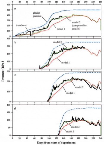
Fig. 14. Fitting the models (green and red curves) to aquifer pressure (transducer) data (black curve), (a) for the 125m site, (b) for the 85m site, (c) for the 65m site and (d) for the 30m site. Model 1 predictions (red) ignore aquifer compressibility. Model 2 predictions (green) include a compressibility value of mV = 2 × 10⁻⁷Pa–1. The discrepancies between measured and modelled values reveal three important features. Firstly, there is a large mismatch between modelled and measured pressure values during the period of rapid ice loading unless aquifer compressibility is taken into account, and a single compressibility value is a good fit during this phase and the succeeding relatively stable phase. Secondly, after about day 200, the modelled pressure prediction is systematically higher than the measured value, which we interpret as caused by the development of a transverse, low-pressure subglacial channel, up-glacier of the 125m site, that draws down groundwater pressures in the aquifer. Thirdly, the three anomalously high aquifer pressure peaks between about days 160 and 190 at 30m reflect hydrofracturing events in the till very close to this site, which connect the local aquifer very directly with recharge sites at the base of the glacier without the buffering effect of the till.
Table 1. Aquifer characteristics derived by fitting the model to the experimental data. The analysis calculates transmissivity, the product of thickness and conductivity. Conductivity is calculated assuming aquifer thickness to be 50 m. The estimated value of the hydraulic diffusivity (consolidation coefficient, ![]() ) and compressibility, mV, depends on this assumption
) and compressibility, mV, depends on this assumption
Prior to the experiment, we had expected the aquifer to behave passively as a medium of constant transmissibility in discharging the groundwater flux, and did not expect aquifer compressibility to play such an important role in determining aquifer water pressures during ice loading. It is clear, however, that the hydraulic pressure build-up in the aquifer during the first 40 days after glacier overriding is strongly affected by aquifer compressibility, resulting in a cumulative compression of ~1 to 2 m. This enhanced water pressure during ice build-up inevitably leads to increased water pressures in the overlying till, thereby reducing its resistance to glacier movement and potentially enhancing the rate of ice advance. We presume that the very high water pressures during this phase, which can exceed ice pressures at the 65 and 85m transducers, must reflect the absence of easy hydraulic connections above these sites and the glacier surface, which would have released water pressures. This is consistent with the fact that the most rapid phase of loading is associated with the passage of an uncrevassed compressional wave front (Fig. 5a).
It is also particularly important to note that the ratio of the plastic (consolidation) to poroelastic (compressibility) components (MV/mV) of 2.6 is very similar to the values observed in laboratory experiments on soil compaction, where MV corresponds to the virgin consolidation (NCL) part of the deformation curve in Figure 13 (e.g. Reference CraigCraig, 1997). It is normally presumed that there is a severe problem of ‘upscaling’ from laboratory measurements to the field, but the large-scale natural consolidation experiment that we have monitored suggests that, in this particular case, there is no significant up-scaling error.
8.2. Recovering the diurnal component of runoff
There is a strong contrast between the hydraulic signatures in the till and the aquifer. The aquifer naturally averages (filters, suppresses) the high-frequency components of influx whilst till transducers show a highly fluctuating signal at the highest sampling frequency. However, it is difficult to extract information about the dynamics of diurnal pressure fluctuation in the till from our model because we are limited to measurements of surface water production every 24 hours (Fig. 9). We have therefore attempted to recover the diurnal component of runoff using the recorded differences between aquifer and till pressures, given by Equation (26). Knowing the pressure difference across the till and the loading history for the whole dataset allows us to find Fourier components at all frequencies and to resolve Equation (26) with respect to runoff, R. The main difficulty is having to combine experimental results from different transducers, which makes inversion of runoff data non-unique. Two attempts were made to invert runoff data from the 125m transducer for days 0–96.75, from the 85m transducer for days 97–132.75, and from the 30m transducer for the rest of the observation period. It proved impossible, however, to produce a single inversion that matched the runoff data for the whole period. It was possible to obtain a good match between inverted runoff and experimental data for the period after day 137 when the mean value of pressure difference across the till is conserved. We suggest that for the earlier period the movement of crevasses over the site caused local variations in the intensity of runoff (e.g. Fig. 10a, insert). Better results were obtained using synthetic runoff data, where the diurnal fluctuations are added as a simple harmonic signal with maximum at 1800 h:
where R is the measured (24 hour) water production rate.
8.3. Till conductivity, compressibility and dynamics
A relationship between runoff and water pressures in the till permits us to infer till properties such as hydraulic conductivity, compressibility, the penetration depth of the diurnal runoff pulse and the characteristic timescale of response. The best data for this exercise are those from the 30m transducer for which there is a complete set of till and aquifer pressures. The best match between model and field data is shown in Figure 15. There is a very satisfying agreement for aquifer and till pressures, with discrepancies (1) around day 140, possibly caused by variations in ice profile and velocity that were not picked up by our periodic observations, and (2) between days 165 and 190, possibly the consequence of hydrofracturing events in the aftermath of high-water-pressure events, as well as (3) the general decline in actual compared with modelled pressures after day 200, that could be a consequence of local channel development (see section 11.2). The data do not show a phase delay caused by till filtering, implying that the characteristic time for the till is less than 6 hours, the pressure sampling period. Figure 16 shows similar results for modelling pressure variations in the till at the 65m (mid-till), 85m (mid-till) and 125m upper transducers. There are no obvious phase delays in these data that allow us to put upper limits on the volume compressibility coefficients, mV, and, consequently, lower limits on the hydraulic diffusivity (consolidation coefficient, cV). We cannot therefore directly infer the compressibility of the till from these data, but we have assumed that it is similar to that which can be inferred, using our theory, from the data presented by Reference Boulton, Dongelmans, Punkari and BroadgateBoulton and others (2001a) where the water-pressure monitoring frequency is sufficient to show depth-dependent phase lags. Figure 17 shows these results, together with a theoretically expected diurnal water-pressure variation and a well-constrained coefficient of volume compressibility, mV ≈ (7.5 ± 2.5) × 10–7 Pa–1. The best fit shown in Figures 15–17 permits us to infer the till properties shown in Table 2.

Fig. 15. (a) Simulated pressures (red curve) for the till transducer at 30m compared with measured pressures (black curve). (b) Simulated and measured pressure drop across the till, showing the maximum gradients at times of maximum water influx (Fig. 9). The till transducer failed to register for about 60 hours after day 220.

Fig. 16. Comparison between mid-till transducer data (black curve) and modelled mid-till water pressures (red curve) at (a) 125 m, (b) 85m and (c) 65 m.

Fig. 17. High-frequency measurements made by till and aquifer transducers reported by Reference Boulton, Dongelmans, Punkari and BroadgateBoulton and others (2001a), showing the phase lag between transducers that the mini-surge data cannot show because of the low frequency of measurement. Modelled pressures for the mid-till transducer are also shown.
Table 2. Inferred characteristics of the till at transect sites. The final row shows values calculated from the data of Reference Boulton, Dongelmans, Punkari and BroadgateBoulton and others (2001a). The values in parentheses are what would be expected if the compressibility of till were the same as in their article. The inequalities follow from the fact that our measurements are insufficiently frequent to reveal a phase shift at the depths of our transducers. It is noticeable that at 65 and 85 m, the till was sufficiently thick (see Fig. 7) to prevent the diurnal cycle from penetrating to the base of the till

We are surprised by the small range of deduced values of hydraulic conductivity, which we suggest reflects the facts that (i) the till matrix is generally massive and homogeneous, apart from large boulders within it, and lacks the large-scale granulometric variability of stratified sediments, and (ii) the well-mixed sandy/silty matrix favours a narrow range of conductivity compared with clay-rich tills whose clay content often varies considerably over short distances. We are also surprised that trench excavation and refilling appear not to have introduced permeability variations during remoulding, suggesting that trench excavation and refilling did not produce significant sorting and that glacial consolidation and deformation overprinted any consolidation during trench refilling.
Laboratory consolidation tests conducted on a basal till sample collected from a trench dug into the margin of Storglaciaren, northern Sweden, by Reference Baker and HooyerBaker and Hooyer (1996) gave estimates of compressibility coefficients of 1–5 × 10⁻⁷ Pa–1 in the effective pressure range 100–300kPa. This agrees well with our mean in situ average of ≈7.5 × 10⁻⁷ Pa–1 under effective pressures between 0 and 50 kPa.
Using the till thickness along the transect from Figure 7, interpolating between the values of conductivity shown in Table 2 for the transducer sites and using a constant value of compressibility (mV = 7.5 × 10⁻⁷Pa–1), we have modelled the till response for every 5m interval along the transect. Figure 18 shows the results for hydraulic diffusivity and characteristic time. It shows the effect of the finer-grained till characteristic of the inner part of the transect (Fig. 8) in slowing the response time. In principle, the till in the inner part of the transect will show a greater tendency to undrained loading and instability than that in the outer part.

Fig. 18. Inferred till properties along the transect. Conductivity and compressibility were deduced by theory from the water-pressure and water-production data; these were used in turn to infer the penetration depth of the diurnal wave and the characteristic penetration time. Properties in (b-e) reflect the finer grain size of the till in the inner part of the transect (see Fig. 8).
9. The Role of Conductivity and Compressibility in Till Dynamics
It is clear from Equations (4) and (5) that the hydraulic behaviour of tills will be strongly affected by their hydraulic conductivity, K, and coefficient of volume compressibility, mV. The former is largely determined by granulometry, the latter by mineralogy and granulometry and both by the state of consolidation. Conductivity is determined by the size, density and tortuosity of interconnected voids, and ranges from about 10–6 m s–1 for sandy tills to about 10–11 m s–1 for clay-rich tills. Compressibility is determined by mineralogy (a matrix of readily deformable, plastic clay, or hard elastic quartz grains) and grain-size distribution (which determines packing geometry) and varies from about 10–8 Pa–1 for highly consolidated sands to about 10–5 Pa–1 for weakly consolidated clays. The state of consolidation can vary from a lightly consolidated state (relatively high conductivity and high compressibility) to a heavily consolidated (or overconsolidated) state (relatively low conductivity and low compressibility).
The coarse-grained till at Breiðamerkurjökull belongs to a till type that has high K/mV values, and includes many of the tills produced by erosion of hard igneous and metamorphic rocks, including those that occupy the shield areas that underlay the central area of the Pleistocene ice sheets in North America and Europe. They contrast strongly with the fine-grained tills derived from the sedimentary rocks flanking the shield areas in North America and Europe, which underlie the marginal zones of the ice sheets, and which exhibit low permeability and high compressibility (low K/mV values).
In order to understand some of the consequences of this contrast, we explored the behaviour of tills of different conductivity/compressibility by modelling their response to diurnal fluctuations in water pressure or recharge. The key parameters that determine behaviour are:
T T – the characteristic response time of the till to fluctuations in pressure on its boundaries, given by T T = d2/cV, where d is till thickness and cV is hydraulic diffusivity.
δ – the penetration depth of a water pulse into the till for a given frequency, given by
where ω is the pulse frequency.
Thus, for till at the Breiðamerkurjökull experimental site, where K is about 6 × 10⁻⁷ms–1 and compressibility about 7.5 × 10⁻⁷ Pa–1, the response time to diurnal fluctuations for a till 1m thick is about 0.15 days (3.6 hours), which explains why no phase lag is apparent in our data, for which the sampling interval is 6 hours. The dimensionless parameter, ωT t, for a diurnal frequency (ω = 2π d–1), is less than 1, and the penetration depth for a diurnal pulse will therefore be at least 1.4 m, explaining why a diurnal signal penetrates to the base of the till. If there had been a smaller conductivity and/or larger compressibility, so that ωTt = 8, the penetration depth would only be 0.35 m, and the diurnal signal would not extend to the base of the till. We therefore do not expect the Breiðamerkurjökull tills to suffer sustained undrained loading and the sustained mechanical instability to which this would give rise when the diurnal signal does not penetrate through the till (Equation (B15), Appendix B). Evidence of the effect of these contrasting modes of till behaviour on glacier movement will be published elsewhere.
Figure 19 shows the results of simulations that explore the impact of conductivity and compressibility on characteristic response times and penetration depths for pressure fluctuations on the till surface. Simulations use the range of compressibility and conductivity values shown in Table 3, and are illustrated in Figure 19 in a 4 day window (days 137141), using the influx data shown in Figure 9 and a till thickness of 0.65m (as at the 30m site). Figure 19a shows a simulation of till and aquifer pressures using our lowest inferred value for hydraulic conductivity KT = 1.1 × 10⁻⁷ms–1, and Figure 19a 1 shows the accompanying pattern of diurnal pressure fluctuation through the till. The value of δ/d = 0.79 (Table 3) indicates that the 20kPa pressure fluctuation at the top surface does not penetrate easily through the till.

Fig. 19. (a-f) Modelled patterns of pressure evolution for the till top (black curve) mid-till (red curve) and till base/aquifer roof (green curve) for a till 0.65m thick and for the different combinations of conductivity and compressibility shown in Table 3. The patterns are illustrated for the modelled water-production rates for days 137–141. (a1), (b1) and (d1) show the patterns of diurnal vertical pressure profiles at 6hour intervals during day 141 in the till shown in (a), (b) and (d).
Table 3. Combinations of hydraulic conductivity and compressibility coefficient used in the models shown in Figure 19, and some of the resultant hydraulic properties

Figure 19b is a simulation of a highly inertial till of the same hydraulic conductivity as in Figure 19a and for the same diurnal water-pressure fluctuation on its surface, but in which mV is ten times larger (decreased conductivity would have a similar effect) so that ωT T = 15.7. The penetration depth of the diurnal pulse (δ) is now about a third the thickness of the till. In the non-inertial case (Fig. 19a), diurnal fluctuations almost penetrate to the aquifer roof, but the inertial behaviour of the more compressible till (Fig. 19b) closes the connection between water pressures at the ice-bed interface and the aquifer at diurnal frequencies, even for the relatively permeable till in this simulation. Whereas in the case of the non-inertial till (Fig. 19a), there is a monotonic downwards water-pressure gradient through the diurnal cycle, in the inertial case of Figure 19b, with a long characteristic time of T = 2.5 days, the resultant phase lag creates a transient upward pressure gradient (Fig. 19b 1). Such a reversal of gradient, associated with a significant phase lag, is shown in Figure 17 where the tills were significantly finer-grained and had a higher ωT T value than at the site described here.
Figure 19c-d explore the influence of compressibility on the hydraulic regime. Conductivity is kept constant (KT = 1.1 × 10⁻⁷ ms–1), and runoff rather than pressure on the till surface (an unphysical condition) is prescribed. In Figure 19c, compressibility, mV, is 28.4 × 10⁻⁷Pa–1 (with ωT T = 7.85) and in Figure 19d these increased to 114 × 10–7 m s–1 and 31.4 × 10⁻⁷ Pa–1, respectively, with four effects:
a larger water-pressure gradient through the till,
a stronger water-pressure response at all depths to the rapid initial glacier loading,
greater attenuation (δ/d = 0.55 and 0.18 for Figure 19c and d, respectively; see Table 3) and greater phase delay (T T = 30 and 120 hours, respectively; see Table 3) in the body of the till in response to the diurnal pressure pulse on the till surface,
reduced amplitude of the till-top pressure fluctuation.
Figure 19 e–f explore the effect of changing conductivity. This is decreased from 1.1 × 10⁻⁷ms–1 in Figure 19e to 0.22 × 10⁻⁷ ms–1 in Figure 19f, whilst holding compressibility constant at 14.2 × 10⁻⁷ Pa–1. The resultant increase in ωT T from 3.93 to 19.6 increases the characteristic time, T, from 15 to 75 hours, decreases the penetration depth from 0.5d to 0.23d, and massively increases the pressure gradient. There is no tendency for transient gradient reversal, which only occurs when compressibility is large.
The simulation of the Breiðamerkurjökull transect site in Figure 19a produces a physically realistic outcome. However, increase in compressibility or decrease in conductivity can create sustained excess water pressures at the top of the till which would have made the glacier terminus mechanically unstable (e.g. Fig. 19f), because of the assumption that all basal recharge is discharged by groundwater flow. In such a case we expect that the development of large excess pressures will be inhibited by the development of conduits at the ice-bed interface that will discharge excess water. The simulation in Figure 19a-b, which fixes the water pressure at the top of the till, implicitly makes this assumption.
The model shows that coarse-grained tills of high conductivity and low compressibility adjust rapidly to changes in local pressure, such that instabilities are rapidly attenuated. Fine-grained tills of low conductivity and high compressibility are much more likely to suffer undrained loading, long response times and sustained instability. We suggest, therefore, that mid-latitude ice sheets extending from coarse-grained into fine-grained till zones may have undergone a change in dynamic behaviour, which may be reflected in the highly lobateform of the ice margins in these zones as a consequence of such instabilities compared with those in inner zones (Reference Boulton, Dongelmans, Punkari and BroadgateBoulton and others, 2001a).
It is also important to note that as a till thickens due to progressive deposition, the pressure difference across it will increase, such that at some critical thickness, effective pressures at the top of the till will tend to zero. Consequently, the deposition or erosion of till beneath a glacier will change the degree of frictional coupling, thereby producing a progressive change in the dynamic behaviour of the glacier.
10. Modelling the Consequences of the Meltwater Penetration Rate through an Ice Sheet
The penetration time of surface meltwater at Breiðamerkurjökull is short compared with the frequency of observations. Observations elsewhere show that multiple englacial voids can exist through the whole thickness of a glacier (e.g. Reference Harper and HumphreyHarper and Humphrey, 1995; Reference Fountain, Jacobel, Schlichting and JanssonFountain and others, 2005), so that surface water is able to penetrate to the bed of a temperate glacier in a few hours (e.g. Reference Hock and LeBHock and Hooke, 1993) and so that it can even penetrate to the bed of an ice sheet sufficiently to influence its dynamic behaviour (Reference Zwally, Abdalati, Herring, Larson, Saba and SteffenZwally and others, 2002). However, there is as yet no generally applicable theory about the depth to which water can penetrate, at what rate, how it is influenced by thermal regime and whether there are fast conduction pathways via moulins and slower routes through fractures or even intergranular voids. Nonetheless, we wish to make some general observations about the nature of basal water-pressure fluctuations at the bed of a glacier in response to changes in the rate of surface water runoff, in the expectation that these will influence time-dependent dynamic behaviour.
We know that rapid penetration to the bed is easy in the terminal zone, and assume that it will be less easy with distance from the margin and may effectively cease, possibly blocked by cold ice in the interior. It seems likely that water penetrates through the ice along low-angle passages (Reference Fountain and WalderFountain and Walder, 1998), that reach the bed over distances several times the ice thickness, and more steeply dipping fracture systems (Reference Fountain, Jacobel, Schlichting and JanssonFountain and others, 2005). On the large scale, even low-angle travel is equivalent to local, vertical penetration. Equation (25) defines a parameter (T) that describes the rate of drainage of surface-derived water through the glacier. At Breiðamerkurjökull, we are unable to infer the through-glacier transmission component of this parameter, only that it is less than the 6 hour resolution of measurements. We expect however, that as the ice thickness increases away from the glacier margin, the drainage time through the ice will progressively increase, as will the drainage time through the subglacial system, with the consequence that up-glacier of a particular point, the diurnal cycle of pressure will be attenuated at the ice-bed interface. If longitudinal subglacial drainage is by groundwater flow alone, this will contribute a large part of the total transmission time. If groundwater flows rapidly into longitudinal channels, the impact of groundwater flow on transmission times will be small.
We have modelled the consequences of these processes, shown in Figure 20, for a glacier overlying a 2m thick till with the same conductivity as the 65m site along the Breiðamerkurjökull transect, lying above an aquifer with the same transmissivity as at the site, but with zero time delay in the till. The two-dimensional flowline section of the glacier has a parabolic surface profile, a length of 400km and a summit elevation of ~2000 m. The drainage rate is assumed to vary inversely with the square of ice thickness, and is adjusted such that the diurnal fluctuation is attenuated at an ice thickness of 200 m. The runoff rate from the surface diminishes linearly with altitude. The modelled outcome shows the variation in water pressure at the ice-bed interface resulting from surface water penetration alone. It is assumed that the water-pressure head created by basal melting will be constant and small compared with head variations generated by surface water.

Fig. 20. Modelled Impact of variations of water Infiltrating from the glacier surface on water pressures at the Ice-bed Interface. Input of Infiltration into the glacier of an annual cycle is shown for sites at 50, 200 and 400m in (a), and the input of infiltration over eight annual cycles, Including a 4year period of climate change during which infiltration Is reduced, In (b). The penetration rate of water through the glacier Is assumed to be Inversely proportional to the square of Ice thickness. The progressive attenuation of diurnal, seasonal and annual frequencies reflected In pressure fluctuations at the Ice-bed Interface Is shown In (c-h). The model Includes vertical flow through a subglacial till and horizontal discharge In a sub-till aquifer.
These assumptions produce an up-glacier pattern in which there is an outer zone where diurnal pressure variations are strong (Fig. 20c), but are progressively attenuated, passing in sequence into:
a zone lacking significant diurnal fluctuations but showing fluctuations reflecting changes of surface runoff over several days/weeks (Fig. 20d) but, as in Figure 20c, no surface-derived impact over the winter season,
a zone with a smoothed reflection of the summer season, and a sufficiently long lag time to show surface-derived pressure variability in mid-winter (Fig. 20e–f), and with the pressure peak displaced by a few months,
a zone in which the amplitude of the annual cycle is much diminished, so that the effect of a lower-than-annual amplitude climate change that takes 4 years is greater than the annual effect, which is lagged by about 6 months (Fig. 20g),
a zone where the annual cycle has been attenuated, but where longer-period climate changes are reflected.
This spatial sequence is also the temporal sequence to which a site suffering progressive glaciation will be subject through time.
We expect that these large-scale patterns, through their varying Impacts on basal friction, will be strongly coupled to glacier dynamics. We expect transmission times to the bed to be related to patterns of Ice conductivity, which reflect patterns of streaming/non-streaming and thermal regime. In addition, large-scale patterns will be related to the subglacial hydraulic architecture.
11. Hydraulic Processes deduced from Model/Data Mismatches
The analytic solution for hydraulic processes generates pressure fluctuations from the runoff series. The results provide an excellent match for most of the data in a way that gives us confidence that it captures the essential behaviour of the system. However, there are some strong and systematic mismatches at particular time periods that suggest the existence of processes not incorporated in the model. Here we identify these mismatches and suggest how they can be interpreted.
11.1. Self-adjustment of aquifer transmissivity through hydrofracturing
The transducers at 125m exhibit intriguing behaviour that we are unable to explain using constant values of aquifer properties. Even though our model 2 (section 8.1 and Fig. 14) fitted the quasi-stationary phase, which incorporates aquifer compressibility, and predicts aquifer pressures well for the period of rapid ice-load increase between about days 85 and 150, there remains a poor fit between about days 37 and 85. During this period, the aquifer transducer shows a very significantly higher water pressure than predicted by either model 1 or 2 (Fig. 14a). The period prior to day 37 is complicated by the upward flow of water near the margin (see section 7.7). We can only interpret this anomaly as reflecting a strong increase in transmissivity between about days 75 and 85.
This becomes plausible if we consider the field observation that fine-grained silty beds commonly occur between gravel lenses within the sub-till outwash sequence (Fig. 4). The change in apparent aquifer properties occurs at about the time of several large runoff-generated pressure spikes. If the effective transmissivity of the aquifer unit at about 125m was limited because of silt aquitards between gravel aquifer compartments, a major water-pressure spike at the ice-bed interface would pressurize the immediately underlying aquifer. This would generate a large potential gradient across the silt bed separating it from the underlying unpressurized aquifer. Consequent hydrofracturing across the silt bed would create new hydraulic pathways, immediately increasing the transmissivity of the aquifer. This might explain the change at about days 75–85, during which newly developing pathways progressively changed aquifer properties. We find that we are able to model the water-pressure behaviour of the aquifer before and after this period if we assume an effective aquifer thickness of 15m beforehand and 50m afterwards (the latter being the thickness inferred from drilling and seismology). We suggest that the apparent increase in effective hydraulic thickness results from the hydrofracturing of conductivity barriers that allow hydraulic compartments to be added to the aquifer.
11.2. Groundwater pressure drawdown due to subglacial channel formation
During days 192–242 (Fig. 14) there is disagreement between model and experiment for the 12, 30 and 65m aquifer transducers (the 125 and 85m transducers were no longer operational). The model predicts a slower general trend of pressure decrease than those clearly seen at the 30 and 65m transducers (Fig. 14c–d) and a higher response to prominent peaks in runoff data. It is impossible to satisfy both data trends because the only physical parameter that strongly affects the aquifer response is the characteristic response time of the aquifer. Decreasing this parameter to account for a rapid seasonal decline in pressures will automatically increase the sensitivity of the aquifer to (i) short influx pulses and (ii) the build-up of water pressure during rapid initial ice loading, thereby increasing the amplitudes of the two prominent peaks.
We suggest that this discrepancy can be explained by local shifts in the mode of subglacial drainage. The retreat of the glacier after the mini-surge ultimately led, in the early 1990s, to a direct connection between Stemmulon lake to the northeast of the experimental site (Fig. 1) and Jökulsárlón, into which it drained. We suggest that across-flow drainage into Jökulsárlón started during this stage, as the glacier stagnated. The anomalously low water pressures during this period could thus be explained by a subglacial channel developing, that ran across the glacier flowline, upglacier of the monitored transect, and intercepted a significant proportion of the aquifer flow, thereby drawing down heads. This would both produce a lower than expected head in the aquifer and a smaller aquifer response to the major rainfall events of days 216 and 234.
11.3. Transient upward water-pressure gradients in the till
Upward head gradients were measured far from the glacier margin during brief diurnal periods. Figure 11b shows the normal state with a downward head gradient and downward flow through the till, with an insignificant diurnal pressure fluctuation in the aquifer. Figure 11c shows a period of strong variations in aquifer pressure, when aquifer pressure peaks temporarily exceed those in the till for periods between 6 and 12 hours in the latter part of the day. In general, the aquifer is recharged by a downward water flux derived from fractures, moulins and crevasses in the glacier. We suggest, however, that where there are no fractures or crevasses in overlying basal ice to provide proximal local recharge at the top of the till, strong increases in aquifer pressure produced by strong recharge from nearby but not overlying crevasses create a transient upward gradient, which decays as aquifer pressures fall again.
11.4. Till hydrofracturing during strong recharge/high-pressure events
The water-pressure gradient across the till normally falls within the range 5–60 kPam–1. However, during some periods of high recharge from the surface, generally associated with heavy rainfall, this can increase to over 100 kPa m–1. On a number of such occasions pressure peaks in the till then decline sharply to values very similar to those in the aquifer (e.g. Fig 11d). They are then sustained at such levels for several days, although showing some fluctuations, before previous values of pressure gradient in the till are progressively re-established.
As has been argued for silt beds in the aquifer in section 8.2, we suggest that the large pressure differences between the till and aquifer, produced by strong recharge from the surface, create hydrofractures in the till. These produce efficient hydraulic pathways between the ice-bed interface and aquifer, which rapidly draw down pressures on the till surface and therefore in the till. This locally enhances the rate of recharge to the aquifer, increasing aquifer pressures. If hydrofracturing is widespread, a general increase of water pressure in the aquifer would result, giving enhanced peaks of diurnal aquifer pressure. If till deformation continued during this phase, the break in till cover produced by hydrofracturing would be progressively sealed, re-establishing the previous hydrological regime. In general, therefore, we might expect hydrofracturing of thin till to be a means of inhibiting large water-pressure differences across the till.
11.5. Water-pressure effect of shearing in the till
Till transducer records tend to show a strong fall in water pressure immediately before they cease recording (Fig. 10). We suggest this reflects dilation associated with shearing in the till, which increases conductivity and reduces water pressure. We believe that transducers cease recording shortly after the till in which they are embedded begins to suffer significant shear deformation. Our records, then, will relate only to non-deforming conditions. This assumption underlies our approach. When deformation of till occurs, we suggest that the potential gradient in the deforming horizons becomes relatively small as a consequence of increased conductivity due to dilation (Reference Boulton, Menzies and RoseBoulton and Hindmarsh, 1987; Reference Boulton and DobbieBoulton and Dobbie, 1993), thereby reducing the effective thickness of the till to which our analysis applies.
When the uppermost of two till transducers fails, pressure at the upper transducer falls below that of the lower. We suggest that as dilation increases and water pressures fall in the upper part of the till as a consequence of shear deformation, pressures in the undeforming body of the till remain high, so that water drains upwards towards the glacier sole. A reversal of drainage that we suggest reflects this process is seen in Figure 17 late on days 253 and 254, when contemporary monitoring of strain (Reference Boulton, Dongelmans, Punkari and BroadgateBoulton and others, 2001b) confirms that the upper part of the till is deforming.
We have attempted to infer the properties of the till along the whole of the transect by considering changes in till thickness and surface elevation, and by assuming that hydraulic conductivity and compressibility can be interpolated between the values at measured sites (Fig. 18a-c). We have then determined the penetration depth for the diurnal wave and the characteristic response time for the till (Fig. 18d–e). Penetration depth shows a pattern that is consistent with grain-size variation along the transect (Fig. 8), with the finer-grained till in the up-glacier part of the transect having a smaller penetration depth and higher characteristic time than the outer part. This part of the till will also be more prone to undrained loading and consequent potential instability.
12. Deducing Hydraulic conditions from Seismic Experiments
Although we are not able to estimate whether and at what rate surface water will penetrate to the bed of a glacier, it is in theory possible to infer hydraulic properties, in time and space, of sediments at the glacier bed. The two key hydraulic properties, conductivity and compressibility, in addition to the shear modulus, govern the nature of the seismic reflection from water-saturated subglacial sediments. In the simplest case of near-vertical reflections, the reflection coefficient of compressional P-waves depends on the acoustic impedances of basal ice and underlying sediments.
For weakly consolidated sediments the acoustic impedance of sediments in the low-frequency approximation is:
where p
T and μ
T are the density and the shear modulus of water-saturated sediments and cW is the compressibility of water (Reference BiotBiot, 1962). Assuming the shear modulus, μ
T, is of the same order as the bulk modulus ![]() as is the case with unconsolidated marine sediments (Reference HamiltonHamilton, 1971), we can see that for our values of till bulk compressibility, mV
≈ 7.5 × 10⁻⁷ Pa–1, the acoustic impedance is totally dominated by the compressibility of water and reduces to:
as is the case with unconsolidated marine sediments (Reference HamiltonHamilton, 1971), we can see that for our values of till bulk compressibility, mV
≈ 7.5 × 10⁻⁷ Pa–1, the acoustic impedance is totally dominated by the compressibility of water and reduces to:

with p T = (1 — ϕ)p S + ϕp W, and is, therefore, a function of porosity alone. Thus, provided some reasonable estimates can be made for the impedance of basal ice, near-vertical reflections of compressional waves exclusively contain information about the porosity of subglacial sediments. This approach has been used to identify deforming and nondeforming basal sediments under Antarctic ice streams using near-vertical (multiple) P-wave reflections (Reference SmithSmith and others, 1997; Reference Vaughan, Smith, Nath and Le MeurVaughan and others, 2003). In an AVO (amplitude vs offset) reflection experiment, additional data concerning the dependence of reflection coefficients of compressional waves were successfully used to estimate the shear modulus of (deforming) basal sediment under Kamb Ice Stream, West Antarctica (Reference AnandakrishnanAnandakrishnan, 2003).
Expressions similar to Equation (39) exist for the problem of reflection of shear waves and for conversion coefficients when an incident compressional wave is partially reflected as a shear wave (and vice versa). These expressions involve different functional coupling between the bulk compressibility, shear modulus and hydraulic properties of the sediments, and are strongly dependent on the angle of incidence and the frequency of seismic signal (Reference Deresiewicz and RiceDeresiewicz and Rice, 1964). We believe that in an appropriately designed AVO-type seismic reflection experiment with three-component records and with a reasonably wide frequency band (~100–200 Hz) all these reflection and conversion coefficients could be evaluated in situ, providing crucial information on hydraulic conditions and material properties of subglacial sediments.
13. Conclusions
In a thick subglacial sedimentary sequence, water pressures at the glacier sole and in immediately sub-sole sediments are determined by the pressure drop along the groundwater drainage pathway, which is a function of the pattern of transmissivity along the pathway and the water flux from the glacier sole. The drainage pathway is therefore a major determinant of the effective pressure at the glacier sole, the frictional resistance to glacier movement and the nature of any basal décollement, either by sliding over the bed or by deformation in the bed. The mini-surge offered an opportunity to monitor the spatial and temporal evolution of pressure evolution in this system in a detail that has not previously been achieved.
13.1. Analysis in the frequency domain
-
1. In order to understand the frequency response of the system to changes in water recharge and ice loading, the hydraulic pathway from the glacier surface to the bed and through subglacial sediments is modelled in the Fourier domain within a framework of three subsystems (ice-till-aquifer) of different linear poroelastic properties, coupled at the ice-till and till-aquifer interface, and with one-dimensional Darcy diffusion of water; it is solved analytically for arbitrary runoff and loading histories. This allows processes to be reformulated in the Fourier frequency domain and resolved analytically at each given location for arbitrary runoff and ice-loading histories. It permits the response of system properties to a broadband signal and changes inboundary conditions to be readily and directly determined, in contrast to the merely ad hoc testing of system properties that can be achieved by finite-element or -difference schemes. The model permits:
the deduction of in situ values of both compressibility and hydraulic conductivity of the till and aquifer directly from the transducer data,
the determination of the ratio of plastic consolidation poroelastic compressibility, which is shown to be similar to that measured in laboratory tests, indicating absence of the normally assumed ‘up-scaling’ problem.
-
2. Major complications are caused by the non-linearity of sediment consolidation (Fig. 13) and by evolving ice-till boundary conditions. We model these non-linear responses of till and aquifer to effective stress with an essentially linear model by considering the frequency-dependent compressibility of sediments (section 7.2.1). The problem of the advancing glacier is resolved by ‘slicing’ the system into a number of vertical cells connected only by horizontal water flow in the aquifer and with independently evolving boundary conditions at the top of the till, caused by the changing glacier load.
-
3. It is unfortunate that the characteristic frequencies of the till and glacier ice were outside (higher than) the 6 hour data frequency available from most transducer signals. This is because of the relatively high conductivity and low compressibility of the coarse-grained till at Breiðamerkurjökull. However, the Fourier approach did demonstrate the existence of a quite unexpected aquifer-scale compressibility that created an important water-pressure wave beneath the advancing glacier terminus.
-
4. We have used our model to explore how fine-grained tills of low hydraulic conductivity, high compressibility and/or great thickness would behave in response to variations in recharge from the glacier. Lower conductivity and higher compressibility inhibit penetration into the till of water-pressure fluctuations so that the signal attenuates at shallow depth, reducing the amplitude of oscillation, increasing the penetration time, increasing the phase lag of the pressure signal with depth and creating the potential for mechanical instability associated with undrained loading, including during rapid increases in loading due to advance of a steep glacier front. The rapid rate of loading associated with the advance of a steep glacier front produces anomalously high water pressures in aquifers as they consolidate, thereby driving up the water pressure in any overlying till. This can be a source of positive feedback to the forward movement of a glacier, and may in part account for the mini-surge. Highly compressible tills may also show transient upward water-pressure gradients as the recharge rate on their upper surface falls. An oscillating water pressure on their upper surface produces periodic, though phase-lagged, reversal of the water-pressure gradient, and could explain periodic oscillations of the décollement surface in tills (e.g. Reference Boulton, Dongelmans, Punkari and BroadgateBoulton and others, 2001a).
-
5. The model is also used to explore the impact of drainage rate of surface meltwater through a glacier on subglacial hydraulics and dynamics. At the Breiðamerkurjökull site, the drainage time is less than the 6 hour frequency of most transducer records, so we are unable to capture its influence on the frequency response of the subglacial hydraulic system. We assume that the drainage time increases under thicker ice, and model how high-frequency components of change in the rate of surface water production will be progressively attenuated under thicker ice. In a near-margin zone, diurnal surface melt fluctuations are reflected in the subglacial hydraulic system. Under increasingly thick ice, higher-frequency fluctuations were progressively attenuated in the subglacial response, so that diurnal responses are progressively replaced by dominantly seasonal, annual and multi-year frequencies. We presume that at some ice thickness, or because of cold ice conditions, there will be negligible surface water penetration to the bed and negligible melt-driven subglacial hydraulic effects, such that water pressures will only be determined by basal melt rates and the drainage pathway. In such a system, the time-scales of water-pressure response will be major determinants of basal dynamic processes. We might therefore expect higher-frequency dynamic effects in marginal zones and lower-frequency effects in inner zones of the same ice sheet. Understanding the whole hydraulic pathway from surface to bed and the effective conductivity of glacier ice is a key issue in understanding the way in which ice sheets may respond dynamically to a warming climate through processes similar to those monitored at Breiðamerkurjökull.
13.2. Analysis in the physical domain
Characteristics of the water-pressure record, and the extent to which they diverge from expectations of the model, are evidence of other important hydraulic processes.
-
1. The surface water production rate, transmissivity of the drainage pathway and fluctuations of ice loading control the state of consolidation of subglacial sediments. The time-dependent variation of ice and water pressure determine the changing state of consolidation of subglacial sediments. The complex hydraulic history at Breiðamerkurjökull produces a complex consolidation history, with previous preconsolidation histories being removed by shear remoulding if rising water pressures exceed a critical value. We deduce from these data that heavy pre-consolidation in a till does not preclude the till having undergone shear deformation at some time during its history.
-
2. It is deduced from the model that a shift in the water-pressure regime during the experiment can only be explained by a major increase in aquifer transmissivity. It is suggested that this occurs because of hydrofracturing in a sequence in which individual lenticular aquifers, reflecting the geometry of glaciofluvial fans, are separated by finegrained, less permeable beds. Rapid loading produced transient strong pressurization of immediately subglacial aquifer lenses, which generated hydrofractures in the finergrained, less permeable beds which separate the upper aquifers from lower, relatively unpressurized aquifers. Hydraulic connection between the aquifers equalized the water pressures between them, thereby increasing the connected transmissivity of the subglacial hydraulic system and producing general water-pressure drawdown.
-
3. Convergence of the pressures in the till and the top of the aquifer occurred immediately after high till pressure peaks at several sites on several occasions, even though diurnal runoff peaks remained high. It is suggested that rapid water-pressure increase on the till top created hydrofractures in the till, making easy hydraulic connections between the glacier sole and the underlying aquifer, thus locally lowering till pressures so that they come close to aquifer pressures. Subsequent shear deformation of till sealed these interconnections, permitting till-top water pressures again to rise well above aquifer pressures.
-
4. Upwelling occurs immediately beyond the margin of the advancing glacier, with water rising through the till from the underlying aquifer driven by a locally strong upward head gradient of up to 25 kPam–1. Observations elsewhere at the margin show that upwelling can be locally strong enough to cause liquefaction and buoyancy in near-surface sediments. Such upwelling, and the reduction in proglacial sediment strength that it causes, may also have facilitated the creation and easy gliding of a push moraine at the advancing glacier terminus. Van der Reference Van der Meer, Kjaer and KrugerMeer and others (1999) have described ‘water escape structures’ in a formerly subglacial aquifer from the glacier Slettjökull in southern Iceland, which we suggest may be former locations of hydrofractures created by pressurized sub-till aquifers.
-
5. The measured water pressures are much lower than those predicted by the model at a late stage in the experiment; this is suggested to be the result of formation of a subglacial drainage channel near the experimental site, which led to general drawdown of groundwater pressures.
-
6. The Breiðamerkurjökull tills are similar in granulometry to most tills lying on the ancient shield rocks in the central areas of the European and Laurentide ice sheets. Our model shows that such tills of high conductivity and low compressibility adjust rapidly to changes in local pressure, such that instabilities are rapidly attenuated, unless the till is very thick. Tills overlying soft sedimentary rocks in the outer zones of the mid-latitude ice sheets show different behaviour, of low conductivity and high compressibility. Modelling the behaviour of such tills demonstrates their potential for undrained loading, long response times and sustained instability. The highly lobate form of ice margins in these zones (Reference Boulton, Hagdorn and HuttonBoulton and others, 2003) may reflect such instabilities.
-
7. The poroelastic theory used in the model to analyze hydraulic effects can also be used to predict seismic responses. We suggest that, building on existing work (e.g. Reference SmithSmith, 1997; Reference AnandakrishnanAnandakrishnan, 2003; Reference Vaughan, Smith, Nath and Le MeurVaughan and others, 2003), the theory could also be used to infer spatial and temporal changes in sediments at the ice-bed interface, including porosity, compressibility and possibly conductivity.
Acknowledgements
The authors are grateful for assistance in the field and laboratory from J. Fleming, K. Dobbie, F. Björnsson, S. Björnsson and E. Jonsson; for assistance with sensors from C. Lussenden and C. Lane; and for comments on the manuscript from A. Smith and an anonymous referee. The work was supported by grant GR3/6898 from the UK Natural Environment Research Council and another from the European Commission.
Appendix A.
Derivation of the Poroelastic Equation For Water-Pressure Dynamics In Compressible Sediments
We write the mass-conservation law for solid and fluid (water) phases of water-saturated subglacial material:

where p s,w and vs,w are the density and velocity of solid and fluid phases, respectively, and ϕ is the porosity. By the density of solid phase we mean the density of mineral grains, not to be confused with the density of (dry) sediments:
The mass-conservation Equations (A1) are not used directly in what follows below, but are necessary to provide an unambiguous definition of the velocities of solid phase and water.
According to the constitutive relationships of linear isotropic poroelasticity (Reference BiotBiot, 1941, 1962), the velocities of solid phase and water are determined by temporal variations in local values of stress field σij and water pressure, p:
where the stress-tensor invariant, σ = 1/3Trσ ij, taken positive for compressional stress, cW and cS are the compressibility coefficients of water and solid grains, and
where p T, defined in Equation (A2), is the bulk compressibility of (dry) sediments.
The dynamic equation for water with the viscous energy-dissipation term reads:
where kis the specific permeability of sediments and p is the dynamic viscosity of water. In the low-frequency approximation, when the inertial term in Equation (A5) and an additional inertial coupling between the solid phase and water are negligible, Equation (A5) reduces to Darcy’s law:

where vf = ϕ(vw – vs) is the filtration velocity of water. Here and in the following we ignore the gravity-induced term pwgz, which can be recovered at any stage when needed. substituting Equation (A6) into the constitutive relationships (A3) and eliminating velocities vs and vw from the final result, we arrive at a closed equation describing the evolution of water pressure in the compressible sediments under applied (external) load σ(t):

An accompanying (deformation) consolidation of sediments is described by Equation (A3) and can be presented as:
where Treij is the absolute dilatation of sediments under variable overload σ and water pressure p given by the solution of Equation (A7).
Appendix B.
Water-Pressure Profile Across The Till
Consider a compressible till layer of thickness d with time-dependent water-pressure distribution p(t, z) satisfying a one-dimensional poroelastic equation,

where water-pressure values at the upper and lower boundaries and stress are arbitrary functions of time: p 0(t), p d (t) and σ(t). Applying a one-dimensional Fourier transform to Equation (B1) with respect to time, we have
where p = p(ω, z) and σ(ω) are the frequency components of water pressure and applied stress. The general solution of the ordinary differential equation (B2) is given by
where the complex eigenvalue,

for positive frequencies, ω, and
for negative frequencies, and δ, the characteristic depth at a given frequency, ω, is given by

The general solution (B3) must satisfy the boundary conditions:
where p0(ω) and pd(ω) are the frequency components of water pressure at the upper and lower interfaces. Substitution of the general solution (B3) into the boundary conditions (B7) yields

This relationship provides a solution for Equation (B2) with given, but otherwise arbitrary, boundary conditions at the upper and lower interfaces and given applied stress. water-flow densities at the upper and lower boundaries are obtained by differentiation of Equation (B2):

and

If the water-flow density, Q0, at the till-top interface is specified as an input in our model then water flow, Qd, at the lower boundary is given by:

When applied to our model, Equation (B11) provides an important relationship for water flow (QTA = Qd ) from the till layer into the aquifer, as a function of water-flow density at the ice-till interface (QI = Q0) and water pressure in aquifer (pA = pd).
To have some useful insight into the physics of water flow in the till layer, consider a simple case when harmonic water pressure p0(t) = cos(ωt) = Re(eiωt), with a diurnal frequency, ω, applied at the top of the till layer, and with the pressure at the bottom (in the assumed underlying aquifer) kept at some constant level, pd = 0. The water-pressure distribution is given then by the solution of Equation (B8) (with σ = 0) in the time domain: sinh A(d — z)

This apparently simple expression is actually the sum of four propagating waves:

where D = 1 — 2e—2Kd cos 2Kd + e-4Kd and we have introduced a wavenumber parameter,
When the till thickness is much greater then the characteristic depth (d ≫ δ) the last three terms in Equation (B13) are exponentially small and our solution is represented by only one (primary) down-going pressure wave,
This diffusion-type wave has a phase velocity given by the dispersion equation

and attenuates in e ffi 2.7 times at distance K–1 = ![]() .
.
When till thickness is comparable with or less than the characteristic depth, δ, the other three waves must be accounted for to satisfy our boundary conditions. The second term in Equation (B13) corresponds to the up-going wave caused by the reflection of the primary down-going wave of Equation (B15). The third term represents another down-going wave which has already been reflected twice (from the bottom and the top of the till layer). Finally, the fourth (up-going) wave has experienced three consecutive reflections (twice from the bottom and once from the top of the till layer). The arguments of cosines include travel-time phase shifts and an additional phase shift (equal to π) caused by a reflection from the bottom of the till. All four of these waves must be accounted for to correctly describe the propagation of water-pressure pulses through a compressible till layer. There is an element of irony that to recover a simple Darcy’s law (when δ ≫ d) one has to account for a fine superposition of four diffusion waves including the rules for their reflection at interfaces.
The similarity of the above to the reflection of seismic waves in layered media is not coincidental. When a seismic wave hits an interface between two different layers of fluid-saturated sediments it generates not only familiar (reflected and transmitted) P- and S-waves, but also a slow compressional P-wave of a second kind. This wave was predicted by Reference BiotBiot (1956) and subsequently confirmed in laboratory and field experiments. This is a highly dispersive and rapidly attenuating compressional wave involving the dynamically coupled motion of solid and fluid phases and is frequently referred to as a Biot wave. For frequencies below the characteristic (Biot) frequency, ω B = ηϕ/pWk, the inertial coupling between the solid and fluid components becomes negligible and the Biot wave degenerates into a wave of fluid diffusion with a dispersion law identical to (B16). Consequently, the representation of pressure pulse dynamics in a compressible till layer as a superposition of four propagating (Biot) waves given by Equation (B13) is a physically correct picture. This provides an interesting connection between subglacial material properties and processes and the reflection coefficients of seismic waves, which can, in principle, be exploited in seismic field experiments.


