


Introduction
In the last three decades, accounting for overdispersion and zero inflation in ecological studies that use count data has become increasingly common (e.g., Welsh et al. Reference Welsh, Cunningham, Donnelly and Lindenmayer1996; Martin et al. Reference Martin, Wintle, Rhodes, Kuhnert, Field, Low-Choy, Tyre and Possingham2005; Warton Reference Warton2005; Sileshi Reference Sileshi2008; Wenger and Freeman Reference Wenger and Freeman2008; Millar Reference Millar2009; Sólymos et al. Reference Sólymos, Lele and Bayne2012; Dénes et al. Reference Dénes, Silveira and Beissinger2015; Blasco-Moreno et al. Reference Blasco-Moreno, Pérez-Casany, Puig, Morante and Castells2019). With count data, overdispersion occurs when the variance of the data is significantly larger than the mean, indicating the model being applied does not appropriately capture the variance in the data (Bliss and Fisher Reference Bliss and Fisher1953). Zero inflation, the presence of excess zeros in a dataset compared with the number of zeros expected under commonly applied count distributions (e.g., binomial, Poisson; Lambert Reference Lambert1992; Heilbron Reference Heilbron1994), is one process that can produce overdispersion. These excess zeros, which can be ecologically real (i.e., true) or produced by non-ecological processes (i.e., false; see Table 1 for paleoecological examples), can change the model that provides the best fit to data and can lead to erroneous conclusions drawn from poorly fit models (MacKenzie et al. Reference MacKenzie, Nichols, Lachman, Droege, Royle and Langtimm2002; Martin et al. Reference Martin, Wintle, Rhodes, Kuhnert, Field, Low-Choy, Tyre and Possingham2005; Blasco-Moreno et al. Reference Blasco-Moreno, Pérez-Casany, Puig, Morante and Castells2019).
Table 1. Potential types of zeros in paleoecological count data with respect to those identified in ecological studies. When taking a sample to evaluate the ecology of a community, ecological processes (i.e., true zeros) and sampling artifacts (i.e., false zeros) can distort the resulting sample relative to the true distribution of specimens or predation events. In paleoecological samples, distortions from additional factors (e.g., preservational bias, time averaging) must also be addressed. *Following Blasco-Moreno et al. (2019). †The possibility of a zero count for a predation trace is predicated on the presence of the prey taxa in the assemblage (ni > 1). When testing a hypothesis on multiple prey taxa, we must also assume the sample from the assemblage is representative of the set of prey taxa that could possibly have been sampled (i.e., were present in the community over the duration of time averaging; see Table 2).
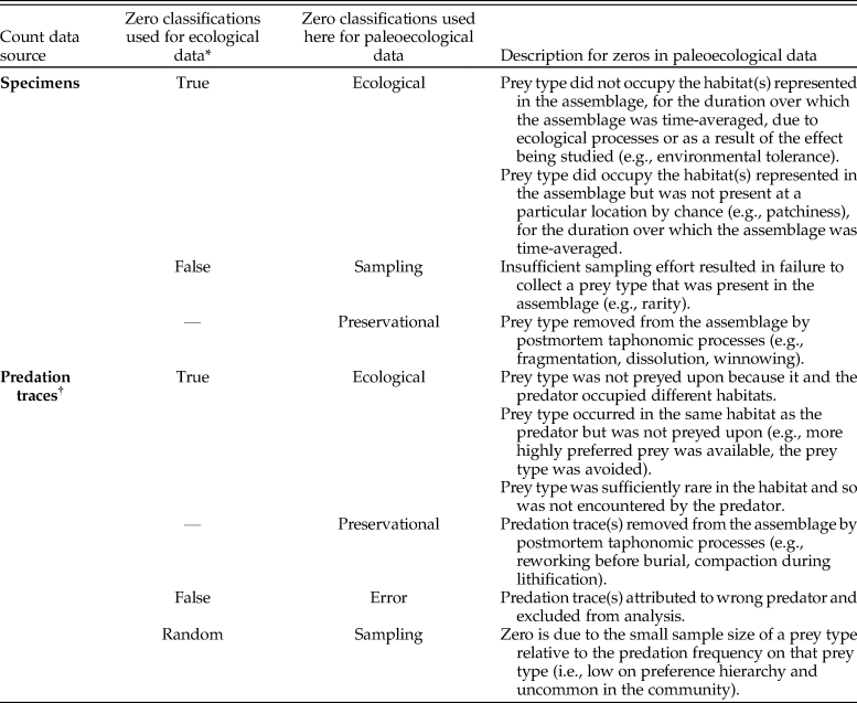
True zeros have ecological explanations, such as a species not occurring at a particular site for an ecological reason (e.g., competitive exclusion) or because, by chance, the species does not saturate its entire suitable range (Martin et al. Reference Martin, Wintle, Rhodes, Kuhnert, Field, Low-Choy, Tyre and Possingham2005)—the latter is similar to a true, “random zero,” described by Blasco-Moreno et al. (Reference Blasco-Moreno, Pérez-Casany, Puig, Morante and Castells2019). False zeros occur when the investigator errs. Errors might include design elements of the study (e.g., attempting to sample a species that is not present in a particular habitat) or failure to observe a species when it is present, which may be common for rare or cryptic species (Welsh et al. Reference Welsh, Cunningham, Donnelly and Lindenmayer1996; Martin et al. Reference Martin, Wintle, Rhodes, Kuhnert, Field, Low-Choy, Tyre and Possingham2005; Wenger and Freeman Reference Wenger and Freeman2008; Blasco-Moreno et al. Reference Blasco-Moreno, Pérez-Casany, Puig, Morante and Castells2019). Accounting for these zeros and differentiating between zeros from different sources can change the results of a study.
Blasco-Moreno et al. (Reference Blasco-Moreno, Pérez-Casany, Puig, Morante and Castells2019) demonstrated this possibility in their examination of the effects of overdispersion and zero inflation on ecological inference. Rather than count data for individuals of different species in a habitat, Blasco-Moreno et al. (Reference Blasco-Moreno, Pérez-Casany, Puig, Morante and Castells2019) used counts of herbivory traces on the flowering heads of four plant species in the genus Senecio, including two native and two exotic species, to evaluate the enemy release hypothesis—that introduced or exotic species will experience less predation compared with native species because they “left behind” their enemies (Keane and Crawley Reference Keane and Crawley2002). Depending on the model used, the Senecio herbivory data could be taken to support or reject the enemy release hypothesis. Using Poisson and zero-inflated Poisson models, Blasco-Moreno et al. (Reference Blasco-Moreno, Pérez-Casany, Puig, Morante and Castells2019) found support for the enemy release hypothesis; however, when utilizing negative binomial and zero-inflated negative binomial models, the hypothesis was rejected. As the zero-inflated negative binomial model was the best-fitting model—it accounted for overdispersion better than the zero-inflated Poisson model, likely because negative binomial models relax the requirement of an equal variance and mean—the authors concluded that the enemy release hypothesis should be rejected. Choosing the correct model to account for overdispersion and zero inflation is critical for reaching correct conclusions from ecological count data.
Just as in ecological studies, count data used in paleoecological studies are susceptible to overdispersion and zero inflation. Though some investigators have begun to consider overdispersion (e.g., Martinelli et al. Reference Martinelli, Kosnik and Madin2015), the potentially misleading effects of zero inflation have not been explicitly addressed. Here we present a hierarchical Bayesian framework consistent with ecological studies as a first step toward addressing overdispersion and zero inflation in paleoecological studies, with consideration for the unique features of paleoecological count data (e.g., time averaging). We apply this framework to a dataset that combines two previously published paleoecological datasets from the Great Barrier Reef—one on molluscan predator–prey interactions (Martinelli et al. Reference Martinelli, Kosnik and Madin2015) and another on the degree of time averaging in an assemblage (Kosnik et al. Reference Kosnik, Hua, Kaufman and Wüst2009; see “A Paleoecological Case Study”)—to demonstrate the potential effects of overdispersion and zero inflation on the results drawn from paleoecological count data.
In addition to applying zero-inflated models in a new context, under a new set of assumptions and conditions, we extend the modeling approach to include zero inflation and overdispersion from two sources: occurrence and abundance of species and occurrence and abundance of predation traces. Though developed in a paleoecological context, this approach is applicable to the study of any predator–prey system in which counts of prey individuals and frequency of predation are each sampled. For example, if it was relevant to the hypothesis they were addressing, the approach presented here could be applied to the data from Blasco-Moreno et al. (Reference Blasco-Moreno, Pérez-Casany, Puig, Morante and Castells2019) to model counts of flowering heads and counts of herbivory traces, allowing for the possibility of Senecio plants without flowering heads.
Count Data in Paleoecological Predation Studies
Studies of predation frequency in paleoecology are subject to a different set of assumptions and conditions than ecological studies (Table 2). By examining accumulations of dead remains, paleoecologists view the end result of the processes they are studying, which have typically played out over decades, centuries, millennia, or longer. With this expanded temporal perspective come two additional sources of variation that must be accounted for by paleoecologists: preservational bias and time averaging (e.g., Fig. 1). Independently, and in association with each other, the effects of preservational bias and time averaging have been the topic of many studies (e.g., Kidwell and Bosence Reference Kidwell and Bosence1991; Flessa et al. Reference Flessa, Cutler and Meldahl1993; Kowalewski et al. Reference Kowalewski, Flessa and Aggen1994, Reference Kowalewski, Goodfriend and Flessa1998; Roy et al. Reference Roy, Miller and LaBarbera1994; Kidwell Reference Kidwell2001, Reference Kidwell2007, Reference Kidwell2013; Goodwin et al. Reference Goodwin, Flessa, Téllez-Duarte, Dettman, Schöne and Avila-Serrano2004; Behrensmeyer et al. Reference Behrensmeyer, Fürsich, Gastaldo, Kidwell, Kosnik, Kowalewski, Plotnick, Rogers and Alroy2005; Olszewski and Kidwell Reference Olszewski and Kidwell2007; Klompmaker Reference Klompmaker2009; Kosnik et al. Reference Kosnik, Hua, Kaufman and Wüst2009; Tomašovỳch and Kidwell Reference Tomašovỳch and Kidwell2010; Olszewski Reference Olszewski2012; Bürkli and Wilson Reference Bürkli and Wilson2017; Dyer et al. Reference Dyer, Ellis, Molinaro and Leighton2018; Smith et al. Reference Smith, Dietl and Handley2019; Sarkar et al. Reference Sarkar, Deole, Paul, Mondal and Saha2020). The consequences of these factors have not been considered, however, with respect to overdispersion and zero inflation as related to paleoecological predator–prey interactions (for a review of existing methods used in paleoecological studies of predation, see Klompmaker et al. [Reference Klompmaker, Kelley, Chattopadhyay, Clements, Huntley and Kowalewski2019]). We focus here on predator–prey interactions in preserved assemblages of recently dead individuals accumulated over the past decade, century, or millennium in the uppermost part of the sedimentary record (i.e., death assemblages; Kidwell Reference Kidwell2009).
Table 2. Common assumptions for time-averaged count data in paleoecological studies of molluscan predator–prey interactions.
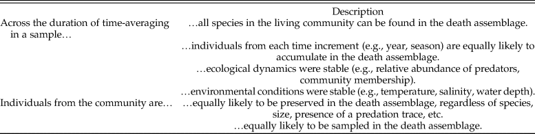
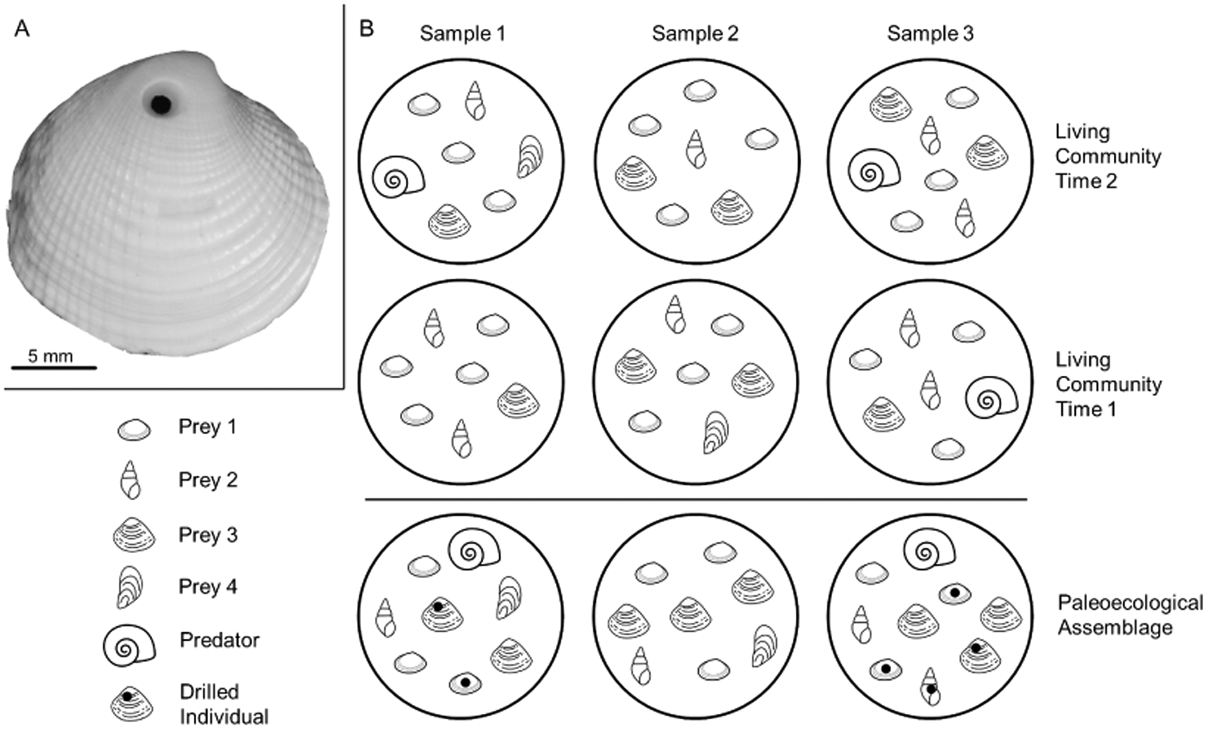
Figure 1. A, Example of a drilling trace made by a naticid predator in its clam prey (personal specimen, J.A.S.). B, An illustrative molluscan community, with three samples taken at two points in time, and the hypothetical time-averaged paleoecological assemblage. The predator is present in sample 3 during time 1 and in samples 1 and 3 during time 2; it is found in the paleoecological assemblage in samples 1 and 3. Time averaging obscures the absence of the predator in sample 1 during time 1. If paleoecological predation frequencies are calculated by pooling data from all samples—including sample 2, where the predator was never present—they would be underestimated because of zero inflation. Counts of individuals are also affected. For example, prey 4 is rare in the living communities but is well preserved in the paleoecological assemblage. With poor preservation, the true abundance of other taxa (e.g., prey 1) is underrepresented in paleoecological samples relative to the living samples. Mollusk drawings from thenounproject.com, with contributors in parentheses: prey 1 (public domain), prey 2 (icon 54), prey 3 (Ker'is), prey 4 (Yu luck), and predator (Juraj Sedlák).
Preservational bias describes the unequal likelihoods that different individuals, or species, will be preserved in a death assemblage based on a variety of factors, which can include body size, habitat, morphology, scavenging, sedimentation rate, or skeletal composition, to name a few. For example, molluscan individuals with small, thin shells may be more likely to be destroyed than individuals with larger, thicker shells. This bias has the potential to prevent individuals, or species, from being preserved in a death assemblage, which can contribute to zero inflation and, thereby, overdispersion. In many cases, a species may not be entirely removed from the record but will instead be represented by fewer individuals. Depending on the sampling strategy employed, these reduced abundances can also generate zeros in samples, particularly when the species was initially rare or has become rare in the assemblage due to preservational bias. Despite this potential bias, death assemblages have been shown to maintain high fidelity to the living assemblages from which they formed, at least with respect to taxonomic composition and rank abundance (e.g., Davis Reference Davis1923; Johnson Reference Johnson1965; Warme Reference Warme1969; Kidwell Reference Kidwell2001, Reference Kidwell2007). With this fidelity in mind, preservational bias can be evaluated as an alternative explanation for observed biotic patterns before drawing conclusions about the pattern or process of interest (e.g., Klompmaker Reference Klompmaker2009; Sime and Kelley Reference Sime and Kelley2016; Smith and Dietl Reference Smith and Dietl2016; Johnson et al. Reference Johnson, Anderson and Allmon2017; Smith et al. Reference Smith, Dietl and Handley2019).
Time averaging describes the accumulation of individuals in an assemblage that lived at different times (e.g., Fig. 1B). Unlike most ecological studies, in which any given individual is known to have lived alongside or interacted with the other individuals in its habitat, individuals in a paleoecological study may have lived decades, centuries, or millennia apart. Time-averaged assemblages tend to have greater richness than the living communities from which they formed because the extended temporal sampling is more likely to capture rare taxa than a survey (i.e., “snapshot”) of a living community (Kidwell Reference Kidwell2002, Reference Kidwell2013; Olszewski and Kidwell Reference Olszewski and Kidwell2007; Bürkli and Wilson Reference Bürkli and Wilson2017) and shifts in populations and habitats over time lead to what is essentially extended spatial sampling (Adler et al. Reference Adler, White, Lauenroth, Kaufman, Rassweiler and Rusak2005; Tomašovỳch and Kidwell Reference Tomašovỳch and Kidwell2009). As such, time averaging in a paleoecological dataset may mask a subset of zeros for species occurrences in a community that would be observed in an ecological dataset, if it were possible to concurrently evaluate a dataset from both perspectives. By virtue of the extended sampling, a time-averaged assemblage can be thought of as the average community from the period over which the assemblage accumulated. Yet, as the averaging smooths out temporal variation in the data, muting short-term trends and patterns (Kowalewski et al. Reference Kowalewski, Goodfriend and Flessa1998), it introduces additional uncertainty and variability with respect to sampling effort. In addition to the inherent uncertainty in estimates of time averaging, variability among samples and among species in the degree of time averaging (e.g., Kosnik et al. Reference Kosnik, Hua, Kaufman and Wüst2009; Kowalewski et al. Reference Kowalewski, Casebolt, Hua, Whitacre, Kaufman and Kosnik2018) unavoidably increases uncertainty in the data, particularly if samples are from more than one locality or time period. Thus, analytically, there is, or at least should be, a cost associated with time-averaged data. To address this uncertainty, paleoecologists typically assume accumulation of specimens in an assemblage occurred at a constant rate and the degree of time averaging is the same across samples, though neither is likely to hold (Holland Reference Holland2016; Tomašovỳch et al. Reference Tomašovỳch, Kidwell and Barber2016; Hopkins et al. Reference Hopkins, Bapst, Simpson and Warnock2018).
The effects of preservational bias and time averaging also apply to counts of predation traces, such as drill holes (for a review of these effects see Klompmaker et al. [Reference Klompmaker, Kelley, Chattopadhyay, Clements, Huntley and Kowalewski2019]). In marine habitats, drill holes are often the result of predation by snails (e.g., Fig. 1A), commonly of the families Muricidae and Naticidae, on other snails and clams. The presence of a drill hole in a shell is taken as evidence that the drilled individual died as a result of predation. In studies of drilling predation, the frequencies upon which prey types—used generically here to refer to genera, species, morphospecies, size groups, or any other grouping of individuals—are drilled (i.e., consumed) are used to evaluate hypotheses relating to both ecology (e.g., prey selection; Kitchell et al. Reference Kitchell, Boggs, Kitchell and Rice1981; Dietl and Alexander Reference Dietl and Alexander1995; Leighton Reference Leighton2003; Chattopadhyay and Dutta Reference Chattopadhyay and Dutta2013; Smith et al. Reference Smith, Handley and Dietl2018a) and evolution (e.g., coevolution and escalation; Vermeij Reference Vermeij1987; Kelley Reference Kelley1989, Reference Kelley1991; Dietl and Alexander Reference Dietl and Alexander2000; Kelley and Hansen Reference Kelley, Hansen, Kelley, Kowalewski and Hansen2003; Mallick et al. Reference Mallick, Bardhan, Das, Paul and Goswami2014; Harper Reference Harper2016; Klompmaker et al. Reference Klompmaker, Kowalewski, Huntley and Finnegan2017).
The effects of time averaging on drill hole counts are similar to those for specimen counts; however, drill holes introduce an additional element on which preservational bias can act. Shells with drill holes may be more susceptible to breakage compared with their undrilled counterparts (e.g., Roy et al. Reference Roy, Miller and LaBarbera1994; Sarkar et al. Reference Sarkar, Deole, Paul, Mondal and Saha2020), though other studies have found a negligible effect of drill holes on preservational potential (e.g., Kelley Reference Kelley, Wisshak and Tapanila2008; Dyer et al. Reference Dyer, Ellis, Molinaro and Leighton2018). The effects of drill holes on shell strength and preservation remain a topic of debate and are likely to vary by prey type, based on other underlying characteristics of the shell (e.g., size, thickness) and depositional environment (e.g., sedimentation rate, wave-energy exposure). If there is an effect, which is very likely for some prey types, it has the potential to contribute to zero inflation in predation count data by removing drill holes from the dataset (Table 1). Given the extent of variability in this effect in terms of prey type and depositional setting, we focus on overdispersion introduced by time averaging and the general process of modeling zero inflation in paleoecological drilling predation studies.
Modeling of Species Abundances and Predation Events
Ecological studies accounting for zero inflation and overdispersion typically consider their effects on a single source of count data (e.g., individuals or predation traces). For example, although Blasco-Moreno et al. (Reference Blasco-Moreno, Pérez-Casany, Puig, Morante and Castells2019) used per-plant counts of flowering heads available to herbivores as an explanatory parameter, counts of flowering heads were not modeled in the same fashion as counts of predation (i.e., herbivory) traces, reflecting the hypothesis they were testing (i.e., zero counts for number of flowering heads would have precluded testing the enemy release hypothesis). The hierarchical Bayesian model we present here includes the potential to model the counts of individuals of different prey types in samples from an assemblage and counts of predation traces on each prey type, while accounting for overdispersion and zero inflation.
Modeling Species Abundances
Count data in studies of paleoecological predator–prey interactions often take the form (xi, yi), where yi is the number of specimens and xi is the number of predation events in sample i of N total samples. In general, sample sizes (yi) are random, and the canonical sampling process is a Poisson process. Yet, in real datasets, counts (yi) rarely obey a simple Poisson model (Hougaard et al. Reference Hougaard, Lee and Whitmore1997). Instead, counts are often overdispersed, potentially due to an excess number of zeros. Similarly, counts of predation events (xi) can be zero-inflated. To draw ecological inferences from such samples, a fundamental question must be addressed: Are these deviations from the Poisson model a result of sampling issues or actual ecological conditions?
We first address this question with respect to sample counts and subsequently apply the developed hierarchical Bayesian framework to a case study. This approach does not obviate traditional maximum likelihood methods (Cameron and Trivedi Reference Cameron and Trivedi2013), which in some applications can provide adequate models. The Bayesian framework allows for more flexible and faithful models, because it better captures sources of variations and the hierarchical (i.e., multilevel) nature of the phenomenon (Gelman and Hill Reference Gelman and Hill2006; Kéry Reference Kéry2010; Korner-Nievergelt et al. Reference Korner-Nievergelt, Roth, Von Felten, Guélat, Almasi and Korner-Nievergelt2015; van de Schoot et al. Reference van de Schoot, Depaoli, King, Kramer, Märtens, Tadesse, Vannucci, Gelman, Veen and Willemsen2021). This approach is particularly useful when data deviate from the ideal Poisson sampling model and violate the assumption that samples represent the same underlying abundance and sampling effort. We consider first the scenario wherein the spatial distribution of specimens is patchy or aggregated owing to a depositional process (e.g., size sorting, winnowing) or an underlying ecological phenomenon. Sample counts would then likely exhibit overdispersion, because the variance of the counts would exceed the mean of the count values. From a Bayesian perspective, this additional variance can be incorporated in a hierarchical model in which the parameter of the Poisson distribution is itself subject to randomness,
 $$\eqalign{& y_i\sim {\rm Poisson}( {\rm \lambda } ) \cr & {\rm \lambda }\sim {\rm Gamma}( {{\rm \alpha }, \;{\rm \beta }} ) } $$
When applying a gamma prior to estimate the Poisson mean, λ, the hierarchical model is equivalent to a negative binomial distribution. There are many reasonable choices for the distribution of λ (e.g., Student's t), which have thick tails (Hougaard et al. Reference Hougaard, Lee and Whitmore1997). However, the gamma distribution is a very flexible distribution capable of taking on many shapes and serves as a versatile model for variation in λ. In addition, the Bayesian approach does not require closed-form formulas for the posterior distribution (e.g., negative binomial). Priors allow for greater probabilities of large outcomes, potentially arising from preservational bias and time averaging. This approach captures the reality that the underlying abundances of each taxon have their own unique distributions and that variation is explained by the probability distribution of λ.
In addition to the underlying variation in the distributions of individual taxon abundances, differences in sampling effort, including the degree of time averaging, can also generate variation. The actual sampling effort represented in a sample is difficult to assess (Olszewski Reference Olszewski2012; Holland Reference Holland2016; Tomašovỳch et al. Reference Tomašovỳch, Kidwell and Barber2016). Among the many processes involved are (1) the “influx” process, which accounts for the biological generation of the specimens themselves (i.e., the underlying abundance) and can vary over time (e.g., Olszewski Reference Olszewski2012); (2) the processes by which specimens are removed through decay, erosion, scavenging, and other processes (e.g., Olszewski Reference Olszewski2012; Tomašovỳch et al. Reference Tomašovỳch, Kidwell and Barber2016); and (3) specimen accumulation over time (i.e., time averaging), which can be variable. For example, estimates of time in assemblages from spatially proximal sediment cores can differ by thousands of years (Kosnik et al. Reference Kosnik, Hua, Kaufman and Wüst2009). These effects are rarely, if ever, quantified in paleoecological studies of predator–prey interactions. Alternatively, variation imparted by these processes can be captured in the model by utilizing more flexible distributions. For instance, if a spatial covariate, like sampling area, were available, variation in the mean could be modeled as,
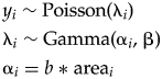 $$\eqalign{& y_i\sim {\rm Poisson}( {{\rm \lambda }_i} ) \cr & {\rm \lambda }_i\sim {\rm Gamma}( {{\rm \alpha }_i, \;{\rm \beta }} ) \cr & {\rm \alpha }_i = b{\rm \;\ast\; are}{\rm a}_i} $$
Going a step further, the time represented in a sample (b) can be modeled to account for uncertainty associated with differences in the degree of time averaging among samples,
 $$\eqalign{& y_i\sim {\rm Poisson}( {{\rm \lambda }_i} ) \cr & {\rm \lambda }_i\sim {\rm Gamma}( {{\rm \alpha }_i, \;{\rm \beta }} ) \cr & {\rm \alpha }_i = b{\rm \;\ast\; are}{\rm a}_i \cr & b\sim {\rm Lognormal}( {\log {\rm \mu }, \;\log {\rm \sigma }} ) } $$
After accounting for this potential underlying variability across samples, the next issue to address is the excess of zeros in the dataset relative to the Poisson sampling process and to determine their origin (Table 1). These zeros can be addressed with a zero-inflated model, allowing zeros from ecological and sampling processes (e.g., Martin et al. Reference Martin, Wintle, Rhodes, Kuhnert, Field, Low-Choy, Tyre and Possingham2005; Wenger and Freeman Reference Wenger and Freeman2008; Blasco-Moreno et al. Reference Blasco-Moreno, Pérez-Casany, Puig, Morante and Castells2019). Such a model is fundamentally a mixture model that allows for a zero to be structural (i.e., ecological), with a certain probability (ωs), or a sampling zero, with one minus that probability,
 $$g( {y_i; \;{\rm \lambda }, \;{\rm \omega }_{\rm s}} ) = {\rm \omega }_{\rm s}I( {y_i = 0} ) + ( {1-{\rm \omega }_{\rm s}} ) f( {y_i; \;{\rm \lambda }} ) $$
where I is an indicator function with a value of one if the condition in the parentheses is true and zero otherwise. The distribution, f, in the second term could be the idealized Poisson distribution or another sampling distribution, including any of the hierarchical types previously described (e.g., eq. 3). With this hierarchical Bayesian approach, sources of uncertainty inherent to paleoecological (and ecological) count data can be better incorporated into ecological inferences.
Modeling Predation Events
As previously described, predation data comprise two counts, (x i, y i), i = 1, …, N, where y i is the number of specimens and x i is the number of predation events in sample i. The number of specimens, y i, can be estimated by Bayesian methods as described in the preceding section. In an idealized setting, counts of predation events (x i) can be estimated as a binomial distribution, where x i are “successes” in y i potential encounters between predator and prey, with a probability of success, p. Parameter p is the predation frequency (e.g., drilling frequency: the number of drilled individuals divided by the sum of drilled and undrilled individuals). This idealized case arises when predatory events are independent of each other and can be written as,
 $$\eqalign{& x_i\sim {\rm Binomial}( {\,p, \;y_i} ) \cr & y_i\sim f( {{\rm \lambda }_i} ) } $$
where the sampling distribution, f, is the idealistic Poisson distribution or, to better account for variation and uncertainty, another count distribution, such as the hierarchical distributions previously described in equation 3. In this case, we assume predation probability is constant in space and time, but that, too, is unrealistic. For example, the predation probability may be a function of predator abundance (e.g., Hansen and Kelley Reference Hansen and Kelley1995; Chiba and Sato Reference Chiba and Sato2014; Stafford et al. Reference Stafford, Tyler and Leighton2015) or biased by differential preservation probabilities (e.g., Walker Reference Walker1989; Klompmaker Reference Klompmaker2009; Smith et al. Reference Smith, Dietl and Handley2019). At the risk of over-parameterizing, we can conceptually elaborate this model to include sample-to-sample variation, as we did with sample counts (e.g., eq. 1), by introducing a distribution on predation probabilities,
 $$\eqalign{& x_i\sim {\rm Binomial}( {\,p_i, \;y_i} ) \cr & y_i\sim f( {{\rm \lambda }_i} ) \cr & p_i\sim h( {{\rm \theta }_i} ) } $$
where h is an appropriate distribution such as beta, which is a standard model for random values between 0 and 1. Moreover, if each sample had a covariate, z i, which potentially influences predation counts (e.g., abundance of predators, preservational bias, water depth), it could be incorporated via logistic regression (Wenger and Freeman Reference Wenger and Freeman2008),
 $$\eqalign{& x_i\sim {\rm Binomial}( {\,p_i, \;y_i} ) \cr & y_i\sim f( {{\rm \lambda }_i} ) \cr & {\rm logit}( p_i) = {\rm \beta }_0 + {\rm \beta }_1z_i} $$
Though data on preservational bias are not assessed in our case study, such data could be incorporated here as a covariate via logistic regression.
It is possible that counts of predation events (x i) are zero-inflated resulting from, for instance, the absence of predators from a habitat due to patchiness during the period over which the sample accumulated, avoidance of certain prey types by the predator, or preservational bias (Table 1). Thus, even when counts of specimens (y i) are positive, it is possible that no predation would have occurred (i.e., x i = 0). It is also possible that a zero is a random sampling artifact, resulting from a small sample size (y i) relative to predation frequency, p (Table 1). As with modeling sample counts, a mixture model captures the probability of excess zeros,
 $$h( {x, \;y; \;p, \;{\rm \omega }_p} ) = {\rm \omega }_pI( {x = 0} ) + ( {1-{\rm \omega }_p} ) {\rm Binomial}( {x; \;p, \;y} ) $$
Allowing counts of predation events (i.e., drill holes) to be zero-inflated enables more precise estimates of the true predation frequency. When estimating predation frequency, the intent is to measure the frequency of attacks when the prey type is “on the menu” and predators are possibly present (i.e., there is a nonzero probability the predatory interaction did or could have occurred). Including all zeros in counts of predation traces from all samples can lead to underestimates of predation frequency. Thus, a zero-inflated model reduces potential downward bias in predation frequency estimation by using a mixture model to differentiate between zeros generated by the phenomenon of interest (i.e., predation) and those originating from other factors (e.g., sampling).
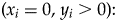
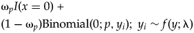
One final component to consider probabilistically is the scenario in which observed specimen and predation event counts are both zero (i.e., x i = 0, y i = 0). This scenario can arise in several ways, including when (1) a prey type count is a false zero (e.g., specimens existed but were not sampled due to preservational bias) and predators were present (i.e., x i = 0 is a sampling artifact); (2) a prey type count is a false zero and predators were not present to drill specimens (i.e., x i = 0 is structural, with an ecological explanation); or (3) a prey type count is a true zero (i.e., ecological) in the sense that specimens were not available for sampling and the predation event count is necessarily zero. For the sake of simplicity, we treat these three possibilities together, with case 1, below. Two alternatives can be applied to estimate predation frequency when specimens are present (y i > 0), without predation (case 2) or with predation (case 3):
1. (x i = 0, y i = 0): ωsI(y i = 0) + (1 − ωs)f(0; λ)
2. $( {x_i = 0, \;y_i > 0} ) \colon $$\eqalign{&{\rm \omega }_pI( {x = 0} ) \; + \cr &( {1-{\rm \omega }_p} ) {\rm Binomial}( {0;p,y_i} ) ;{\rm \; }y_i\sim f( {y;{\rm \lambda }} ) }$
3.
$( {x_i > 0, \;y_i > 0} ) \colon $${\rm Binomial}( {x_i;p,y_i} ) ;{\rm \; }y_i\sim f( {y;{\rm \lambda }} ) $

In these three cases, the distribution f could be the Poisson distribution or any other sampling distribution (eq. 4). As demonstrated above, the model comprising these three cases can become a hierarchical model by allowing parameters λ and p to have indices that vary by sample according to their own distributions (eqs. 1 and 6). Allowing sample-to-sample variation, as facilitated by the hierarchical Bayesian framework, can better account for the uncertainty inherent to ecological and paleoecological datasets and can improve the inferences drawn from them.
Model Evaluation
These hierarchical models can all be fit within the Bayesian paradigm using a probabilistic programming language (e.g., Stan; Stan Development Team 2019). As noted elsewhere, hierarchical Bayesian models, especially as implemented through probabilistic programming languages such as BUGS or Stan, provide flexibility to free the modeler without regard to estimation details (Kéry Reference Kéry2010; Korner-Nievergelt et al. Reference Korner-Nievergelt, Roth, Von Felten, Guélat, Almasi and Korner-Nievergelt2015). In the approach facilitated by sampling methods for posterior distribution estimates, we have the ability to produce true probability statements about the values of parameters, given the data and the model.
One limitation of the sampling approach is the uncertain nature of model ranking. Although many researchers rely on the Akaike information criterion (AIC) to rank scientifically plausible and well-fitting models, the current situation in sampling-based Bayesian estimation is that it is often difficult to select the best model from a set of candidates owing to approximations and estimation error, especially for complicated hierarchical models (see Gelman and Hill Reference Gelman and Hill2006). Model-ranking methods like AIC break down for hierarchical models, because counting the number of parameters is not straightforward. Consequently, similar methods (e.g., the deviance information criterion) have been developed for the Bayesian framework to be used in place of AIC; however, because of their inherent approximations, they have difficulty evaluating competing models (Gelman and Hill Reference Gelman and Hill2006). It is thus generally advised to perform predictive model checking (Gelman and Hill Reference Gelman and Hill2006; Korner-Nievergelt et al. Reference Korner-Nievergelt, Roth, Von Felten, Guélat, Almasi and Korner-Nievergelt2015) to assess model fit and to rely heavily on scientific insight and interpretability for model ranking (Vehtari et al. Reference Vehtari, Gelman and Gabry2017). Posterior predictive checking simulates the fidelity of the model and its fit to the data by drawing random model parameters from their posterior distributions and then simulating data from that random model. If the model fits well, the actual data and simulated data should generate similar histograms and summary statistics. This method is sometimes used as a companion to other model diagnostics (e.g., information theoretic criterion), which may not be informative when sample sizes are too small for the symptotic formulas to hold (Korner-Nievergelt Reference Korner-Nievergelt, Roth, Von Felten, Guélat, Almasi and Korner-Nievergelt2015). We follow this approach to model checking (see Supplementary Material).
A Paleoecological Case Study
To illustrate the potential effects of overdispersion and zero inflation in paleoecological studies, we analyzed data from Martinelli et al. (Reference Martinelli, Kosnik and Madin2015) using the framework developed in the preceding section. We did not reevaluate the hypotheses presented in Martinelli et al. (Reference Martinelli, Kosnik and Madin2015). Instead, we used their data to highlight sources of variation that may confound many, if not all, paleoecological studies using count data and to illustrate a statistical framework to address these sources of variation. All analyses used the Bayesian programming language Stan (Stan Development Team 2019) called from within the R statistical programming environment using the package rstan (Stan Development Team 2018). All code and data are available in the Supplementary Material.
The data from Martinelli et al. (Reference Martinelli, Kosnik and Madin2015) are from replicate samples of the molluscan living and death assemblages in three lagoons at One Tree Reef, in the southern Great Barrier Reef. Fifteen sampling sites were included, with seven from the first lagoon and four from each of the others. Four replicates were collected at each site from a 0.25 m × 0.25 m area on the seafloor, to a sediment depth of 10 cm. Sampling was repeated four times throughout the year, resulting in 16 samples from each site. We only assessed the death assemblage samples here—one sample from each site was processed in most cases, because death assemblages often contain more individuals than the living assemblage. When death assemblages contained relatively few individuals, additional samples were included, resulting in different sampling efforts for some sites (see Supplementary Table 1). All processed samples were sieved on a 4-mm mesh, and all individuals were identified to the species level. Occurrences of predatory drill holes were also recorded, and predation frequencies were calculated.
As is the case for most paleoecological studies, including our own work, Martinelli et al.'s (Reference Martinelli, Kosnik and Madin2015) original study did not assess the degree to which the death assemblages were time-averaged, which was a source of variation of interest in our analysis. To remedy this lack of temporal context for our illustrative case study, we applied time-averaging data from Kosnik et al. (Reference Kosnik, Hua, Kaufman and Wüst2009), which were collected from molluscan death assemblages at Rib Reef on the Great Barrier Reef. The data from Kosnik et al. (Reference Kosnik, Hua, Kaufman and Wüst2009) are from two 125-cm-deep cores of the seafloor sediments. In the top 25 cm of the cores, shells were typically younger (i.e., from the last several years or decades) than those from the deeper part of the core, and from 25 to 125 cm, shell ages were well mixed throughout. Time averaging was on the scale of thousands of years, but varied considerably between cores (e.g., ages for Abranda casta ranged from 2 to 1019 years in core 1 compared with 4 to 4670 years in core 2; see Supplementary Fig. 1).
We acknowledge these two datasets are from disparate locations on the Great Barrier Reef and may not truly hold any bearing on each other. Ideally, time-averaging data should be collected from the same samples being analyzed to evaluate (paleo)ecological hypotheses; however, there is a paucity of such studies. Thus, because our objective was to develop an analytical framework with the capacity to incorporate data on time averaging and illustrate the potential biasing effects of overdispersion and zero inflation, we proceeded with this combined dataset for illustrative purposes.
Overdispersion Analysis
In the data from Martinelli et al. (Reference Martinelli, Kosnik and Madin2015), specimen counts varied greatly for many species (e.g., 19–925, Pinguitellina robusta; see Supplementary Table 1). This variance resulted in overdispersion, as noted by the authors: “the ratio of model residual deviances to residual degrees of freedom tended to be greater than one, indicating overdispersion” (p. 820). The counts for P. robusta are representative of those common in death assemblage samples and were used here to illustrate the presence of overdispersion and incorporation of greater uncertainty into a paleoecological model.
Sample-to-sample differences in counts likely arose from ecological processes (e.g., patchiness, aggregation) due to underlying environmental conditions (e.g., water depth, temperature) or variation in sampling effort. We fit four models to these count data and evaluated goodness of fit using a posterior predictive check (Table 3). Without information on environmental conditions (i.e., a covariate), any differences are effectively random. To account for this randomness, we allowed the mean count to vary more than permitted in a simple Poisson distribution by including a gamma prior (i.e., eq. 1):
 $$\eqalign{& y_i\sim {\rm Poisson}( {\rm \lambda } ) \cr & {\rm \lambda }\sim {\rm Gamma}( {{\rm \alpha }, \;{\rm \beta }} ) } $$
Alternatively, differences in sampling effort owing to sampling area and time averaging can be incorporated. First adding sampling area, we fit a model in which the area is presumed to be the main driver of specimen counts, while also allowing for extra variation from a gamma distribution:
 $$\eqalign{& y_i\sim {\rm Poisson}( {{\rm \lambda }_i} ) \cr & {\rm \lambda }_i\sim {\rm Gamma}( {{\rm \alpha }_i, \;{\rm \beta }} ) \cr & {\rm \alpha }_i = b{\ \rm \ast \ are}{\rm a}_i} $$
Because the mean of the Gamma(αi, β) distribution is αi/β, estimates of αi and β will track expected counts through λi.
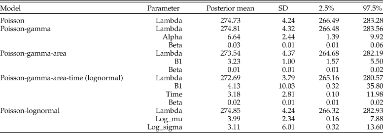
Table 3. Parameter estimates for the posterior predictive check assessing goodness of fit for models of counts for Pinguitellina robusta. Estimates for each parameter of the various models are given as the posterior mean, with associated standard deviation (SD) and 95% credibility regions (2.5%–97.5%).
To this point, the analysis could apply equally to ecological or paleoecological data. As the Martinelli et al. (Reference Martinelli, Kosnik and Madin2015) data are paleoecological, it is also reasonable to assume some degree of time averaging is contributing to the variation in the counts, which, in the absence of data from Martinelli et al.'s samples, we drew from Kosnik et al. (Reference Kosnik, Hua, Kaufman and Wüst2009). As discussed above, the accumulation of a death assemblage is complicated and includes random influx of individuals, a suite of temporally variable processes that remove individuals, and right-censorship of the data (Tomašových et al. Reference Tomašovỳch, Kidwell and Barber2016). Without auxiliary data on accumulation, we could not infer from first principles how specimens actually accumulated in the sample. Consequently, we applied the assumption that time averaging is positively correlated to specimen counts (Tomašovỳch and Kidwell Reference Tomašovỳch and Kidwell2010). By extension, we necessarily also assumed that rates of specimen accumulation exceeded rates of specimen removal and that both rates were relatively constant over the period of time averaging (Table 2). Reflecting the uncertainty associated with these assumptions, we used a general, flexible model to capture variation in sampling effort.
To incorporate the uncertainty introduced by time averaging into the model, we fit a lognormal distribution to the time-averaging data for A. casta—formerly known as Tellina casta; a confamilial of P. robusta—from two cores sampled by Kosnik et al. (2009; see Supplement 1). We used the parameters of this fitted lognormal,  $\hat{{\rm \mu }} = 6.64, \;\hat{{\rm \sigma }} = 1.99$, as a prior to simulate average accumulation time-interval lengths in the model,
 $$\eqalign{& y_i\sim {\rm Poisson}( {\rm \lambda } ) \cr & {\rm \lambda }\sim {\rm Gamma}( {{\rm \alpha }_i, \;{\rm \beta }} ) \cr & {\rm \alpha }_i = b\;\ast\; {\rm are}{\rm a}_i{\rm \;\ast\; time} \cr & {\rm time}\sim {\rm Lognormal}( {6.64, \;1.99} ) } $$
As with the previous model, the mean of the Gamma(αi, β) distribution is αi/β, such that estimates of αi and β track the expected counts through λi. In essence, the model implies sampling area and accumulation time drive the count process, with extra variation captured by allowing each sample its own gamma distribution. Because there are no environmental covariates in the model, this last model assumes original abundances were constant across sampling areas.
We used posterior predictive model checking to evaluate the models (Table 3). The variation in sample sizes was not adequately explained by the Poisson or Poisson gamma models. The model using sampling area as a covariate fared better, because area increased with sample size, but still not enough to capture the larger sample sizes. The model with a lognormal prior did not offer much improvement over the area covariate model owing to the significant amount of count data that overwhelmed the prior.
In the absence of covariates that more completely capture sampling effort, of which time averaging is a critical component, it is difficult to fully model the sampling process and expose the underlying abundance. The plausible lognormal fit to the age data from Kosnik et al. (Reference Kosnik, Hua, Kaufman and Wüst2009) suggests time averaging could be an important driver of sample-size variation. That is, time-averaging data collected from the same specimens analyzed for predator–prey interactions may better explain the variance and improve the model fit. Likewise, adding data on alternative explanatory variables (e.g., environmental factors, preservational bias) as covariates (e.g., eq. 7) would reduce the reliance on assumptions (e.g., Table 2) and likely improve model fits. Data issues notwithstanding, the framework developed here allows for the incorporation of accumulation processes into estimates of specimen counts, representing a step forward in paleoecological analytical methods.
Zero-inflated Predation Frequencies
In paleoecological studies, drilling predation frequencies are typically calculated by pooling the number of drilled and undrilled individuals across samples and dividing the total number of drilled individuals by the total number of individuals. Intuitively, when the pooled number of individuals is high the estimate of predation frequency can be interpreted more confidently and when the pooled number of individuals is low (e.g., n < 30) there is greater uncertainty in the estimate. The uncertainty is increased when the number of individuals in each unique sample is low. It is this latter case we evaluated here, using the snail Notocochlis gualtieriana from the Martinelli et al. (Reference Martinelli, Kosnik and Madin2015) study as an example (see Fig. 2 for analysis of species with at least 15 total individuals; see also Supplementary Fig. 2).
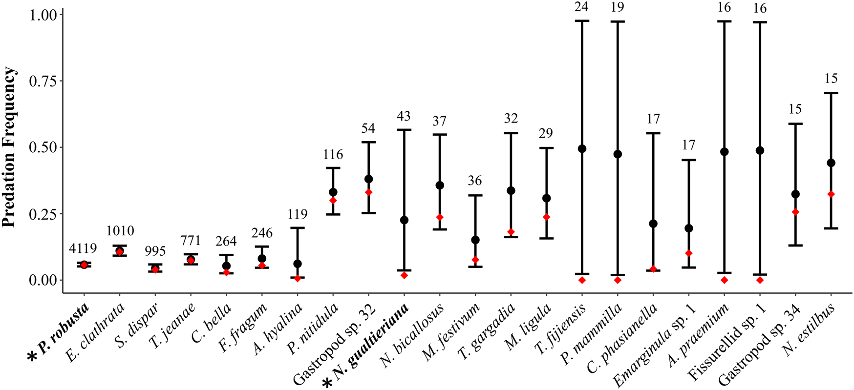
Figure 2. The effect of zero inflation on estimates of predation frequency. Species are sorted by sample size in decreasing order from left to right, with specimen counts given above the black bars for confidence regions—species with fewer than 15 individuals were excluded (see Supplementary Fig. S2). Black circles represent predation frequencies accounting for zero inflation (p), with 95% confidence regions (black bars). Red diamonds represent predation frequencies for each species estimated with the traditional calculation (number of drilled individuals divided by the total number individuals in each sample). Data from Martinelli et al. (Reference Martinelli, Kosnik and Madin2015). Asterisks on the x-axis with bolded taxon names indicate the two species, Pinguitellina robusta (far left) and Notocochlis gualtieriana (central), discussed in the main text.
In 5 of the 15 sampled sites, no N. gualtieriana specimens were reported. Specimen counts ranged from 1 to 12 in the 10 sample sites where N. gualtieriana was found. In total, only one N. gualtieriana specimen was drilled, indicating that the predatory interaction was ecologically plausible (see Supplementary Table 2). Pooled together, N. gualtieriana was represented by 43 individuals and, following the traditional calculation, was drilled with a frequency of 0.02. This traditional approach does not address the abundance of zeros in the drilling data; in 9 of 10 samples, no N. gualtieriana specimens were drilled. Thus, we fit a zero-inflated mixture model to the data. As the dataset is small and apt to support a variety of models, we fit a single, ecologically plausible model and evaluated it with posterior predictive checking: (i.e., eq. 8)
 $$h( {x, \;y; \;p, \;{\rm \omega }_p} ) = {\rm \omega }_pI( {x = 0} ) + ( {1-{\rm \omega }_p} ) {\rm Binomial}( {x; \;p, \;y} ) $$
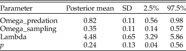
In this case, the model fit was good, as the posterior predictive check indicated the actual and simulated data had similar histograms and summary statistics (Table 4). With the zero-inflated model, the predation frequency (p) was estimated to be 0.24, indicating considerable underestimation with the traditional approach. The difference is largely the result of allowing for the second zero-generation process in the model. Indeed, a majority of the zeros in the dataset for N. gualtierianna were determined to be true, structural zeros (i.e., the absence of predation had a probable ecological explanation).
Table 4. Parameter estimates for the posterior predictive check assessing goodness of fit for the model of predation counts on Notocochlis gualtieriana. Predation frequency (p) is estimated using the hierarchical Bayesian model. For comparison, the predation frequency estimate using the traditional method (number of drilled individuals divided by the total number of individuals) is 0.02. SD, standard deviation.
Considering all species in the death assemblage with at least 15 individuals (Fig. 2), we found that predation frequencies for several other species (e.g., Atys hyalina, Tellina gargadia) were also underestimated due to zero inflation. In general, species can be put into three groups: high abundances and few ecological zeros (left side of figure); moderate pooled abundances but low abundances in each sample and many ecological zeros (right side of figure); and species with low pooled abundances precluding meaningful inference (not shown in Fig. 2; see Supplementary Fig. 2). The differences between estimates of predation frequencies calculated with the traditional approach and with a zero-inflated model are most pronounced in the middle group. Ecologically, this is plausible when considering the distribution and abundance structure of species in communities. Often, a subset of species in the community will be highly abundant and these species will be heavily preyed upon, numerically, as a function of their abundance. Even so, those abundant species may rank low in a predator's preference hierarchy, and less common taxa may exhibit greater predation frequencies per capita in places and times when the predator and prey overlap (Kitchell et al. Reference Kitchell, Boggs, Kitchell and Rice1981; Hansen and Kelley Reference Hansen and Kelley1995; Martinelli et al. Reference Martinelli, Kosnik and Madin2015; Smith et al. Reference Smith, Handley and Dietl2018b). Predation of this second variety is better represented with a zero-inflated model than with the traditional approach applied in paleoecology.
Discussion
On the surface, paleoecological and ecological count data appear to be nearly identical. Many, if not all, metrics applied to ecological count data can also be applied to paleoecological count data, and both types of data are susceptible to zero inflation and overdispersion. Yet, because of preservational bias and time averaging, paleoecological count data are inherently more variable and carry a greater degree of uncertainty than ecological count data (Fig. 1B). In paleoecological studies, these effects are often addressed by making assumptions (Table 2) or assessed as alternative explanations for observed biological patterns. That is, they are either ignored a priori or discounted after the fact—including in our own previous work. The hierarchical Bayesian framework developed here allows for the effects of time averaging and preservational bias to be included while examining potential biological processes and patterns. In essence, the analysis treats variation introduced by preservational bias and time averaging as if it was overlain on the variation inherent to the ecological processes, which is more realistic.
Analytically, incorporation of these sources of variation is important when choosing the model to represent the data. Each model carries assumptions about how the data, and thereby community or assemblage, are structured. As demonstrated in the case study here and in previous studies (Martin et al. Reference Martin, Wintle, Rhodes, Kuhnert, Field, Low-Choy, Tyre and Possingham2005; Wenger and Freeman Reference Wenger and Freeman2008; Blasco-Moreno et al. Reference Blasco-Moreno, Pérez-Casany, Puig, Morante and Castells2019), whether the underlying assumptions of the models are valid (e.g., variance equal to the mean in a Poisson distribution) can influence the model that best fits the data. Despite the similarities in ecological and paleoecological count data, it is often more challenging to validate these assumptions in paleoecology because of the long-acting processes at play. Consequently, there is more uncertainty in paleoecological inferences. By accounting for uncertainty from time averaging within a hierarchical Bayesian framework, our case study suggests that those inferences can be improved.
To address this uncertainty with respect to zero inflation and overdispersion, estimation of the potentially confounding sources of variation (i.e., time averaging, preservational bias) is a necessity. Though it was hitherto rare for such data to be collected and integrated into a single paleoecological study, the risk of misinterpreting data and drawing erroneous conclusions makes the incorporation of such data paramount. Whereas the effect of preservational bias will tend to be unidimensional (i.e., removal of specimens resulting in zero inflation), the effects of time averaging are more complicated.
As treated here, time averaging can be thought of as a temporal sampling window. Whether an assemblage accumulated over a decade, century, or longer, the end result is a set of individuals that have been “sampled” from the entire period of time (Fig. 1B). In a dataset composed of such samples, time averaging has two potential effects: (1) reduced zero inflation because of extended temporal sampling capturing rare events and occurrences and (2) increased uncertainty because of sample-to-sample variability in the extent of time averaging. The first effect, capture of rare occurrences, is often viewed as a positive attribute, as it allows for a more complete accounting of the average state of the community. Typically, the “rare occurrence” being captured is that of a rare species in a community (e.g., Prey 4 in Fig. 1B), which results in greater richness of death assemblages (Kidwell Reference Kidwell2002, Reference Kidwell2013; Olszewski and Kidwell Reference Olszewski and Kidwell2007; Bürkli and Wilson Reference Bürkli and Wilson2017). This effect likely can also be extended to rare predation events. For example, if a prey type is ranked low in a predator's preference hierarchy, predation on this prey type may only occur with very low frequencies (e.g., <1%). Yet, because time averaging captures rare occurrences, it would be more likely to find a rare instance of predation in a death assemblage than in a survey of a corresponding living community. Thus, this first effect likely reduces zero inflation, and thereby overdispersion, with respect to the occurrence of species in an assemblage and the incidence of rare predation events.
The second effect, increased sample-to-sample variability in extent of time averaging, increases the uncertainty in inferences drawn from the count data. Though it is often assumed, individuals likely do not accumulate in an assemblage at a constant rate, especially individuals of different species (Kosnik et al. Reference Kosnik, Hua, Kaufman and Wüst2009; Olszewski Reference Olszewski2012; Holland Reference Holland2016; Tomašovỳch et al. Reference Tomašovỳch, Kidwell and Barber2016; Kowalewski et al. Reference Kowalewski, Casebolt, Hua, Whitacre, Kaufman and Kosnik2018). Many factors (e.g., bioerosion intensity, sedimentation rate, water chemistry, taxonomy) affect the inclusion of specimens in an assemblage, and they vary through space and time. Ecological communities also vary through space and time, with various correlations to the factors affecting preservation. Consequently, the living community from one year may contribute more individuals to a death assemblage than the living community from the next year or the living community 10 years later. Though paleoecologists do regularly standardize one aspect of sampling effort by taking volumetrically controlled samples (i.e., bulk samples) from a locality, the true sampling effort represented by a paleoecological sample is uncertain, because the assemblage itself accumulated variably. For example, in the two cores used here to estimate time averaging, there was a fourfold difference in the range of ages of individuals—core 1 ranged from 2 to 1019 years and core 2 ranged from 4 to 4670 years—despite samples being taken from the same general area (Kosnik et al. Reference Kosnik, Hua, Kaufman and Wüst2009). If one is only comparing samples from the same assemblage, there is a greater likelihood that the temporal sampling effort will be similar; however, when comparing assemblages from different times and places, time averaging may vary substantially (Kowalewski et al. Reference Kowalewski, Goodfriend and Flessa1998; Kosnik et al. Reference Kosnik, Hua, Kaufman and Wüst2009; Ritter et al. Reference Ritter, Erthal, Kosnik, Coimbra and Kaufman2017). Incorporation of time averaging into analyses of count data can improve model fits by accounting for this additional variability.
The Issue of Preservational Bias
The assumptions used commonly by paleoecologists to account for the effects of preservational bias are not unlike assumptions applied in ecological studies. For example, in surveys of ecological communities, it is common to assume that all individuals have equal and independent detection probabilities (Martin et al. Reference Martin, Wintle, Rhodes, Kuhnert, Field, Low-Choy, Tyre and Possingham2005; Wenger and Freeman Reference Wenger and Freeman2008). Intuitively, we know that this is unlikely to hold because of variations in size, morphology, behaviors, and life histories, among others. The paleoecological assumption that all individuals are equally likely to be preserved in an assemblage, and thus equally likely to be found in a paleoecological sample, is based on the same general sampling principles. Both assumptions rest on the shared premise that the sample taken is representative of the potential individuals that were available (i.e., living in the community) for sampling. Convenient as it is to make this assumption in paleoecological studies, several studies on drilling predation have cast doubt on its validity, at least when drill holes are involved (e.g., Roy et al. Reference Roy, Miller and LaBarbera1994; Klompmaker Reference Klompmaker2009; Smith et al. Reference Smith, Dietl and Handley2019; Sarkar et al. Reference Sarkar, Deole, Paul, Mondal and Saha2020).
Unlike the extent of time averaging, which can be estimated using temporal information (e.g., carbon isotopes) extracted from specimens and sediments, preservational bias describes the preclusion or removal of information (i.e., individuals) from a sample. It is an estimate of what has been lost and, because it is derived from assumptions and generalized patterns based on characteristics of preserved specimens, cannot be known with absolute certainty. Furthermore, each prey type in a sample may be affected differently by preservational processes based on size, habitat, and other factors. For example, Kosnik et al. (Reference Kosnik, Hua, Kaufman and Wüst2009) examined the age distributions of four taxa in a death assemblage and, within the same core, found shell half-lives (i.e., the time it takes for half of the shells of a species to be removed from the death assemblage) of 574 (Abranda), 630 (Natica), 925 (Ethalia), and 1229 (Turbo) years. In a core taken nearby, the half-life was 171 years for Abranda and 552 years for Turbo. This variability in cores taken from the same area suggests a need to account for preservational bias, for which Kosnik et al. (Reference Kosnik, Hua, Kaufman and Wüst2009) suggested a composite shell durability score from shell density, thickness, and shape, to predict shell half-life. The uncertainty introduced by time averaging likely compounds the uncertainty from preservational bias, because the processes contributing to preservational bias are also variable in space and time.
Preservational bias is onerous to estimate and likely contributes to zero inflation and overdispersion in paleoecological count data. The general assumptions, used in many studies, that individuals accumulate at a constant rate and accumulation exceeds removal (Table 2) may not hold (Olszewski Reference Olszewski2012; Holland Reference Holland2016; Tomašových et al. Reference Tomašovỳch, Kidwell and Barber2016). When estimates on preservational processes are available, they can be readily incorporated into the framework developed here (eq. 7). This hierarchical mixture model approach is well suited to incorporate the uncertainty inherent to paleoecological data by identifying and beginning to account for zeros introduced by ecology and preservation.
Conclusions and Future Work
Overdispersion and zero inflation are common in paleoecological count data and, just as is the case with ecological count data (MacKenzie et al. Reference MacKenzie, Nichols, Lachman, Droege, Royle and Langtimm2002; Martin et al. Reference Martin, Wintle, Rhodes, Kuhnert, Field, Low-Choy, Tyre and Possingham2005; Blasco-Moreno et al. Reference Blasco-Moreno, Pérez-Casany, Puig, Morante and Castells2019), can lead to misinterpretation of data and erroneous conclusions. We illustrate this potentiality using data on drilling predation (Martinelli et al. Reference Martinelli, Kosnik and Madin2015) and time averaging (Kosnik et al. Reference Kosnik, Hua, Kaufman and Wüst2009) from molluscan death assemblages as a hypothetical case study. The hierarchical Bayesian framework we present here to analyze these data builds on the foundation of overdispersion and zero-inflation analyses in the ecological literature by allowing for two sources of related count data (i.e., counts of species abundance and predation traces) to be modeled together, rather than from a single source (i.e., counts of species abundance or predation traces) of count data. To the best of our knowledge, this study is the first attempt to incorporate the effects of overdispersion and zero inflation into inferences about predation drawn from paleoecological count data—related methods have been used in occupancy (e.g., Liow Reference Liow2013) and fossilized birth–death (Barido-Sottani et al. Reference Barido-Sottani, Aguirre-Fernández, Hopkins, Stadler and Warnock2019; Warnock et al. Reference Warnock, Heath and Stadler2020) models in paleontology. Though this represents a step forward, it is only a single step among many to be taken to produce more confident ecological interpretations of species' interactions in the paleontological record. Indeed, because of the longer timescales involved, these issues may be more pervasive in fossil assemblages than in the relatively young death assemblages considered here.
Further work is needed to better account for and understand the complex relationships between overdispersion and zero inflation, and preservational bias and time averaging. Most pressingly, there is a need for paleoecological studies that incorporate estimates of time averaging and preservational bias in the process of drawing inferences, rather than ignoring or dismissing them in advance or checking for their influence after the fact. Without doing so, the long-standing assumptions applied in paleoecology (Table 2), and used here, will continue to limit the inferences drawn from paleoecological data. Collecting data on each of these elements in a single study represents a considerable challenge and deviation from standard practice in the discipline, where these elements are often considered in isolation. With a better accounting of these effects, and thereby uncertainty in paleoecological data, the barriers to integration of data across timescales can more readily be overcome. That is, ecological data and paleoecological data will be more readily comparable, enabling more seamless hypothesis testing across timescales.
It is also important to note that the framework developed here is not one-size-fits-all but can be modified to accommodate different hypotheses. Whereas it would be appropriate to apply the entire framework to evaluate zero inflation in a study examining predator preference, when only ecologically plausible interactions have bearing on the hypothesis (e.g., prey type 1 is preferred over prey type 2), it may not be appropriate in a study evaluating mortality risk. Because mortality risk is considered from the perspective of the prey population, a zero for drilling predation should not be excluded, for example, when testing a hypothesis on the relative importance of multiple selective agents (e.g., durophagous predation, drilling predation, abiotic stress). Still, even in the latter case, accounting for uncertainty from time averaging and zero inflation from preservational bias remains relevant, and the models can be adjusted accordingly. As has been stated elsewhere (e.g., Blasco-Moreno et al. Reference Blasco-Moreno, Pérez-Casany, Puig, Morante and Castells2019), the treatment of zeros in a dataset should be determined by the hypothesis being tested.
Though our case study focused on the effects of overdispersion and zero inflation in paleoecological studies of drilling predation, the modeling framework we developed can be applied to a variety of ecological and paleoecological contexts. Indeed, paleoecological studies examining other predation traces (e.g., repair scars from failed attacks by crabs on clams and snails) or morphological features (e.g., spines, ribs) would likely also benefit from analysis with a hierarchical Bayesian framework that accounts for overdispersion and zero inflation in multiple types of count data. The same is true of ecological studies that make use of more than one type of count data. For example, these methods could be applied to studies of disease prevalence in communities with respect to abundance in the community, the frequency of herbivory on different species in a community with respect to abundance, or any similar set of data with multiple count variables. Ecological and paleoecological inference stand to benefit by more completely addressing the potential for misinterpretation of data caused by overdispersion and zero inflation.
Acknowledgments
We thank the editors, J. Crampton and J. Huntley, and the reviewers, J. Bauer and P. Novack-Gottshall, for their comments on an earlier version of this article, which improved its quality.
Data Availability Statement
Data and parameter estimates used in the hypothetical case study (Supplement 1) and code and data files required to reproduce results (Supplement 2) can be found at https://doi.org/10.5281/zenodo.4814590.


 Open access