


Introduction
Global circulation models (GCMs) are consistent in predicting that “greenhouse gas” -induced climate warming will be particularly marked at northern high latitudes, especially in winter (Hansen and others, 1981; Cao and others, 1992; Manabe and others, 1992; McGinnis and Crane, 1994; Lynch and others, 1995). For a doubling of atmospheric CO2 from the present level of 340 ppmv, GCMs predict a warming of 8–12°C for areas above the Arctic Circle in December, January and February (Houghton and others, 1990, 1992). Summer warming is, however, predicted to be less than 4°C in the same areas. Summer precipitation is predicted to increase slightly, while little change is expected in winter precipitation. Attempts to simulate the response of the mass balance of Arctic glaciers to climate changes such as these have utilised both energy-balance and degree-day mass-balance models (Huybrechts and others, 1991; Oerlemans and Fortuin, 1992; Bøggild and others, 1994). Results generally suggest that the increase in melting due to summer warming is likely to exceed any increase in accumulation, such that Arctic glacier mass balance is likely to become more negative as climate warms. Winter warming and the associated reduction in seasonality of the thermal climate are generally considered to have no significant impact on mass balance (Braithwaite and Olesen, 1993).
The mass-balance response of Arctic glaciers to climate warming is complicated by the process of superimposed-ice formation, which must therefore be incorporated in mass- balance models (Reeh, 1991; Oerlemans and others, 1993). Superimposed ice forms at the base of the snowpack on Arctic glaciers, where percolating meltwater refreezes on contact with underlying cold ice (Baird, 1952; Arnold, 1965; Koerner, 1970; Palosuo, 1987; Jonsson and Hansson, 1990). Ice formed in this way has to be melted again before it can run off from the glacier surface, effectively reducing the net ablation produced by a given input of energy to the glacier surface. Under current climatic conditions, superimposed-ice formation is an important process of accumulation on high-Arctic glaciers, and it is the dominant form of accumulation on many ice masses in the Canadian high Arctic, including the Meighen, Barnes, Bylot and Devon Ice Caps (Baird, 1952; Koerner, 1970). Thus, changes in the rate of superimposed-ice formation might be expected to play an important role in mediating the relationship between climate change and the mass balance of these glaciers.
Typically, mass-balance simulation models treat the formation of superimposed ice in a highly schematic fashion. A common approach is to set some limit to the thickness of superimposed ice which can develop (Reeh, 1991; Huybrechts and others, 1991; Letréguilly and others, 1991). This is done using a parameter, P-max, which is the proportion of snowpack water equivalent which forms superimposed ice at a given site. In general, P-max has been assigned a value of 0.6, largely on intuitive grounds, although some field studies do support a value of this order. For instance, Wolfe (1995) obtained a value of 0.67 from studies on Quviagivaa Glacier, Ellesmere Island, Northwest Territories, Canada. In all studies of which we are aware, the value of P-max is held constant, even when climatic boundary conditions are altered substantially from those of the present day.
Since these previous attempts to incorporate superimposed-ice formation in ice-sheet models seem oversimplified, this paper attempts to develop a simple yet rational way of calculating P-max and incorporates the calculation into a mass-balance model. The model will then be used to determine how P-max might vary as climate changes, and to evaluate the likely effect of changes in P-max on the mass balance of a high-Arctic glacier. Particular consideration is given to the possibility that winter warming and reduced climatic seasonality might reduce P-max, and thus have a negative impact on mass balance, even in the absence of significant summer warming.
Relationship Between Superimposed-Ice Formation And Climate
In analyzing the relationship between superimposed-ice formation and prevailing climate, our goal is to develop a model which can be readily applied to areas and time periods for which the availability of both meteorological data and high-resolution measurements of near-surface ice temperatures is limited. Such a model is essential if it is to be readily incorporated into existing mass-balance and ice-sheet simulation models.
Our approach follows that of Ward and Orvig (1953), who developed a method which successfully predicted both the timing and thickness of superimposed-ice formation on the Barnes Ice Cap, Baffin Island (70°00 N, 74°00’ W). This method assumes that, at the start of the period of superimposed-ice formation, glacier ice to a depth of 14 m is isothermal at the mean annual air temperature (consistent with the findings of Hooke (1976)). Once the snowpack has become isothermal at 0°C, meltwater can then percolate to the base of the snowpack where it refreezes and releases latent heat. This heat is conducted into the underlying ice, raising its temperature. This continues until a temperature gradient has been established whereby minimal water must refreeze to maintain a 0°C near-surface ice layer. There-after, runoff occurs from the glacier surface. According to Ward and Orvig, the thickness of superimposed ice, X (cm), formed after a given time period, t (s), is given by:
where α is the thermal diffusivity of ice (0.011 cm2 s–1) and A is a constant given by:
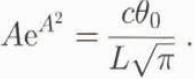
Here c is the specific heat capacity of ice at 0°C (2097 J kg–1 °C–1), L is the latent heat of fusion of ice (333.5 KJ kg–1), and θ 0 is the temperature at 14 m depth (i.e. the mean annual air temperature).
Values of A were found for θ 0 ranging from –2° to –20°C (at 2°C intervals) by iterative solution of Equation (2). Values of X associated with each value θ 0 were then found by assuming that t = 864 000, based on results of Wolfe (1995), who found that the rate of superimposed-ice accretion on Quviagivaa Glacier fell to a negligible level after an average of 10 d in the 1993 melt season. Although it is recognised that the duration of the period of superimposed-ice formation may vary with changes in mean annual air and near-surface ice temperature, field observations indicate considerable variability in this parameter, even between sites with very similar air temperatures (Wolfe, 1995). Since our goal is to develop a simple means of predicting P-max, which can readily be incorporated into mass-balance and icc-sheet simulation models (which operate at coarse spatial and temporal resolution), we have neglected this effect in the current model. For similar reasons we have also neglected the influence of variable rates of meltwater supply, surface slope and surface roughness on the formation of superimposed ice. Although these effects should be incorporated in a full physical model of superimposed-ice Formation, such a model would need to be formulated at higher resolution than the current model. Thus, accepting the above value for t, the relationship between X and θ 0 becomes:
This relationship can be used to predict the distribution of superimposed-ice thickness formed across a glacier during a single melt season, and thus to estimate the appropriate value for P-max at each location:
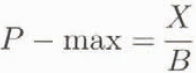
where B is the local snowpack water equivalent (cm H2O) at the start of the melt season. To do this, it is necessary to know the mean annual sea-level air temperature (MASLAT) and snowfall at the site, and to be able to estimate the variation of mean annual air temperature and snowfall with elevation using appropriate lapse rates. This step utilises assumptions which are already used in both energy-balance and degree-day mass-balance simulation models.
An important result of Ward and Orvig’s analysis is that superimposed-ice formation is sensitive to changes in mean annual temperature. Since winter warming, such as is predicted by GCMs for Arctic areas under doubled CO2 scenarios, will increase mean annual air (and 14 m ice) temperatures even in the absence of summer warming, it may thus have a significant impaci on mass balance through a change in the rate of superimposed-ice formation. To explore the possible consequences of this effect for glacier mass balance, we undertook a series of mass-balance simulations for a glacier in the Canadian high Arctic on which field evidence suggests superimposed-ice formation is an important process of accumulation.
Study Site
John Evans Glacier is a large valley glacier located at 79°40’ N, 74°00’ W, on an unnamed peninsula south of Dobbin Bay, eastern Ellesmere Island. It has a catchment area of 220 km2, of which 74% is glaciated. The glacier spans an altitudinal range of 98–1453 m, but 62% of the ice surface area lies between 600 and 1100 m. In this study, mass-balance modelling focused on a 63.5 km2 subsection of the main trunk glacier, which spans the full elevation range of the glaciated part of the catchment.
During the period 1951–94, the mean elevation of the glacier’s equilibrium line is estimated to have been around 900 m (A. Arendt, unpublished results from degree-day mass-balance simulations). Most of the glacier’s surface area thus lies within ± 300 m of this elevation. In 1988–89, an automatic weather station located in Allman Bay, 5 km south of the glacier, recorded a mean annual temperature of–17.3°C (personal communication from G Henry, 1994), some 0.4°C lower than was recorded at the Atmospheric Environment Service weather station at Alert (82°30’ N,

Fig. 1. P-max as a function of elevation for different MASLAT. Snow depth is held constant at depths measured at John Evans Glacier (1995).
62°20” W) over the same period. Accumulation on the glacier, B (cm w.e.), was determined from snow pits at 100 m elevation intervals from 100 to 1100 m at the end of the 1994–95 accumulation season. It increased with elevation (Z) according to the relationship B = 0.0082z + 10.48 (r 2 = 0.75, p <0.001). Sea-level accumulation was 1.22 times that recorded at Alert over the same period.
Mass-Balance Model For John Evans Glacier
Mass-balance simulations for John Evans Glacier were performed by prescribing an accumulation distribution across the glacier and calculating ablation using a version of the energy-balance model described by Arnold and others (1996). This model is driven by hourly meteorological measurements (incoming solar radiation, air temperature, 2 m wind speed, relative humidity). It calculates the one-dimensional surface energy balance for each cell in a digital elevation model (DEM) as the sum of five individual components: the sensible and latent heat fluxes between the atmosphere and the glacier surface, the net short-wave and long-wave radiation fluxes, and the conductive heat flux into the glacier. The melt rate in each cell is determined from the net energy balance. The model uses a DEM (25 m grid size) of the glacier surface and surrounding topography to account for the effect on solar-radiation receipts of slope, aspect and shading of the glacier surface by surrounding topography. The DEM was constructed photogrammetrically from 1:60 000 aerial photographs taken in 1959. It was checked by GPS surveys in 1995, which showed elevation changes of < ± 10 m since 1959.
Several changes were made from the model described by Arnold and others (1996), in order to make it applicable to high-Arctic glaciers. The parameterized treatment of the change in surface albedo over time was altered to follow Van de Wal and Oerlemans (1994). The effect of changes in cloud type (observed twice daily) on long-wave radiation fluxes was incorporated, following Ohmura (1981). A term for the conductive heat flux into the glacier was added. This was assigned a constant value of 0 W m–2 during the period of superimposed-ice formation, thus implicitly assuming that all latent heat released during superimposed-ice formation was conducted into the glacier, and a constant value of 17.6 W m–2 for the rest of the ablation season (following Konzelmann and Braithwaite, 1995).
The formation of superimposed ice was incorporated into the model as follows. At the start of each run, an estimate of P-max was made for every grid cell in the DEM using Equations (3) and (4). After the onset of melt in a given cell, snowmelt was stored as superimposed ice until the thickness of superimposed ice formed equalled B x P-max. Thereafter, snowmelt was allowed to run off. Once all snow had been removed from a cell, the superimposed ice was melted. Only after all the superimposed ice had melted was the underlying glacier ice allowed to melt, resulting in a negative specific mass balance for the cell. Full details of the model as implemented are given in Woodward (1996).
Results
P-max
To determine P-max, all simulations used the winter 1994–95 relationship between water equivalent accumulation and elevation. Simulations of the glacier’s mass balance under current climate conditions used MASLAT of – 17.8°C (the 1951–94 mean at Alert) and a temperature-elevation lapse rate of 0.004°C m–1 (as measured in northern Greenland by Bøggild and others (1994)). For the purposes of this study, simulations for warmer climates assumed an increase in MASLAT that was attributable solely to winter warming. This made it possible to evaluate the possible impact of winter warming on superimposed-ice formation and mass balance, whilst allowing the energy-balance model to be driven with meteorological data collected under current summer climate conditions.
The predicted variation of P-max with elevation and MASLAT is shown in Figure 1. At low temperatures, P-max decreases with increasing elevation because the accumulation rate increases more rapidly with elevation than does the thickness of superimposed ice. At temperatures close to zero, however, P-max increases with elevation because superimposed-ice thickness increases more rapidly than accumulation rate.
Mass balance
For the purposes of simulating the mass balance of John Evans Glacier under current climatic conditions, the energy-balance model was run using hourly meteorological measurements collected by an automatic weather station located at the snout of the glacier during the period 16 June–7 August 1994. This period covered most of the 1994 ablation season. Other aspects of the model set-up were as described above. An annual mass loss from the catchment of 11.8 x 10⁶ m3 (specific mass balance = –0.19 m a–1) was predicted, with an equilibrium-line altitude (ELA) of 1147 m.
The model was rerun ten times, keeping the accumulation distribution and summer meteorological conditions constant, but increasing MASLAT in increments of 1°C to simulate the effect of winter warming on superimposed-ice formation. Specific mass balance decreased almost linearly at a rate of approximately 0.008 m a–1 (or 4.2% of calculated present-day mass balance) per °C of warming (Fig. 2), while the ELA rose to 1239 m for a warming of 10°C (Fig. 3). The impact of winter warming on superimposed-ice formation in grid cells at 450 and 1050 m elevation is shown in Figure 4. As the climate warms, the period of superimposed-ice

Fig. 2. Increased volumetric runoff from the catchment with increasing MASLAT (as a result of decreased superimposed-ice formation).

Fig. 3. Specific mass balance with changing MASLAT, showing decreased superimposed-ice formation (averaged for every cell per 100 m elevation band). The control run for present-day climate is represented by a mean annual air temperature of–17.8° C.
formation gets shorter, the maximum thickness of superimposed ice is reduced, and net balance at the end of the melt season is decreased. On a glacier-wide scale, the net effect of winter warming is to reduce both the area in which superimposed ice accumulates and the thickness of ice formed within this area. As expected from the hypsometry of the glacier, the largest increases in runoff volume are predicted for the area between 600 and 1100 m in elevation (Fig. 5).
Conclusions
A method has been developed for predicting the fraction of snowpack water equivalent (P-max) which forms superimposed ice from the mean annual air temperature at a site. If patterns of snow accumulation are held constant and mean annual air temperature increases, P-max will decrease. For John Evans Glacier, the direction of the relationship between P-max and elevation changes from negative to positive as temperature increases.
GCMs predict significant greenhouse-gas induced climate warming at northern high latitudes. Even if this is concentrated in winter and no summer warming occurs, formation of superimposed ice is likely to be reduced on many high-Arctic glaciers. This will have a negative impact on mass balance. For John Evans Glacier, simulations suggest that specific mass balance is likely to decrease by about 0.008 m a–1 for every degree increase in mean annual temperature

Fig. 4. Curves showing increased ablation (m) with decreased depths of superimposed ice formation (a) 450 m and (b) 1050 m.

Fig. 5. Net ablation vs elevation with warming MASLAT, resulting in decreased superimposed-ice formation.
brought about by winter warming. This would be sufficient to raise the ELA by about 100 m for a 10°C increase in mean annual temperature. Although this effect is relatively small in comparison to the changes which might result from increased summer temperatures (we estimate that a 1°C rise in winter temperature comprises 7% of the decrease caused by a similar rise in summer temperature), it is nonetheless significant, given the very low specific mass balance of many high-Arctic glaciers. This is especially true for John Evans Glacier, where it would be superimposed upon an already negative mass balance.
Hitherto, numerical mass-balance models have tended to downplay the possible significance of winter warming for glacier mass balance in areas where winter temperatures are well below freezing. Many have also neglected the influence of temperature- and precipitation-related variations in the rate of superimposed-ice formation on mass balance. Our results emphasise the importance of incorporating the effects of superimposed ice into mass-balance models in a meaningful way if these are to be used to evaluate the sensitivity of mass balance to future climate change or to simulate the long-term response of glaciers and ice sheets to past climate change. The approach adopted here provides a simple means by which this can be done.
Acknowledgements
This work was supported by the Natural Sciences and Engineering Research Council of Canada, Polar Continental Shelf Project, the University of Alberta Central Research Fund and a C-BAR grant from the Canadian Circumpolar Institute. Permission to conduct the work was granted by the Science Institute of the Northwest Territories, and by the people of Grise Fjord and Resolute Bay. We thank G. Henry for providing meteorological data from Allman Bay.


