


1. Introduction
The majority of fresh water resources for communities in the Xinjiang region of Northwest China originate as glacial meltwater in the Tian Shan range (Li and others, Reference Li, Li, Chen and Lu2016a). The Xinjiang region is one of the most arid regions in the world, receiving <200 mm of total annual precipitation (Chen, Reference Chen2014). Studies in the Tian Shan indicate that most glaciers have been retreating rapidly since the end of the Little Ice Age (LIA) and even more rapidly since the 1970s (Aizen and others, Reference Aizen, Aizen, Surazakov and Kuzmichenok2006; Wang and others, Reference Wang2011). Mountain glaciers, especially smaller glaciers, react sensitively to changes in climate (Oerlemans, Reference Oerlemans1994; Haeberli and others, Reference Haeberli, Hoelzle, Paul and Zemp2007; Wang and others, Reference Wang2012; Chen, Reference Chen2014; Li and others, Reference Li2014a). Air temperature is the primary factor controlling the rates of glacial melt in the Tian Shan (Aizen and others, Reference Aizen, Aizen, Surazakov and Kuzmichenok2006; Liu and others, Reference Liu2006; Chen, Reference Chen2014). Xinjiang's regional temperature increase of 0.34°C/decade from 1960 to 2010 surpassed global temperature increases over this period (Chen, Reference Chen2014).
Rising temperatures impact glacial meltwater production, which accounts for over 10% of the river runoff in Xinjiang and has the greatest impact on water resource stability in this region (Li and others, Reference Li, Li and Wang2010; Li and others, Reference Li2014a; Chen, Reference Chen2014). In the mountains, glacial meltwater is a direct fresh water resource (Immerzeel and others, Reference Immerzeel, van Beek and Bierkens2010; Mupenzi and others, Reference Mupenzi and Li2011; Bolch and others, Reference Bolch2012; Chen, Reference Chen2014). In the arid lowlands, glacial meltwater recharges aquifers and regulates river runoff, decreasing during colder, wetter periods and increasing during warm, dry periods, thereby supplying much needed fresh water to desert lowlands during the dry season (Immerzeel and others, Reference Immerzeel, van Beek and Bierkens2010; Bolch and others, Reference Bolch2012). The continued temperature rise predicted for the region poses an urgent threat to the stability of water resources for Xinjiang communities (Li and others, Reference Li2014a).
We investigate past and present glacier changes in the Kaidu River basin of the central Tian Shan mountains. The Kaidu River, the third largest in the Tian Shan, flows into Bosten Lake (Fig. 1), the largest inland fresh water lake in China, which provides water for flood irrigation and protects two populated oases within Xinjiang, directly influencing the Tarim Basin's ecosystem and environment (Chen, Reference Chen2014; Chipman and others, Reference Chipman, Shi, Magilligan, Chen and Li2016). The continued thinning and recession of these glaciers will have significant impacts on the hydrology of the drainage basin and negative ramifications for water availability and resource management, especially in the lower reaches of the river system (Mupenzi and others, Reference Mupenzi and Li2011). The Kaidu River also feeds the Yanqi Basin, which is home to 450 000 people as of 2003 (Li, Reference Li2009). Agricultural production is their main source of income, responsible for over four times the amount of income from industrial production (Li, Reference Li2009). As a result, sustainable agriculture and water resource management are of major interest in the area.

Fig. 1. (a) Location of the study area (red square) in Xinjiang, location and elevation of meteorological stations (pink triangles), and location of other regional glacier change studies (orange circles) referred to in the discussion and Figure 5: (1) Ala Archa; (2) Akshiirak range; (3) Sary-Jaz and Aksu basins; (4) Tekes watershed; (5) Mt. Bogda. Map credits: Esri, HERE, Garmin, FOA, NOAA, USGS and OpenStreetMap contributors. (b) Study area inset showing the three satellite images used for delineation. The 2014 Pléiades image (topmost layer), displayed in true color, covers 35 glaciers in our study area. The 2012 Worldview-2 image (second layer), displayed in false color, and the 1969 panchromatic Corona image (bottom layer) cover all 54 glaciers in our study area. Yellow stars indicate the location of seven LIA end moraines identified.
Despite the significant influence of Tian Shan glaciers on water resources in Xinjiang, field data and long-term monitoring of the glaciers are extremely limited due to the difficulty of access (Wang and others, Reference Wang2012; Li and others, Reference Li2014a). Thus, most studies that investigate glaciers in this region rely on change detection using remotely-sensed data to characterize glacial change and calculate melt rates. These studies are limited in accuracy, especially on shorter timescales, because they are mostly based on the imagery of low or medium resolution (30 m or coarser). In order to address this inadequacy, we investigate the glacier changes in the warming Kaidu River basin using high-resolution (<3 m resolution) satellite imagery.
We examine temporal changes in the surface area, volume and mass of 54 glaciers in the upper reaches of the Kaidu River based on the delineation of glacier margins using high-resolution images from 1969, 2012 and 2014. In addition to active glacier margins, we also delineate the maximum ice extent during the LIA using moraines and other glacial landforms to provide a longer-term record of glacier changes. In the Tian Shan, the LIA glacial advances began in the 15th century and lasted until the beginning of the 20th century (Liu and others, Reference Liu, Sun, Shen and Li2003). We use a range of LIA dates centered around ~430 years ago (~1586 CE) from surface exposure dating of Tian Shan glacier moraines from Li and others (Reference Li2014a) and Li and others (Reference Li2016b) to calculate change rates from this time period. The outermost moraines associated with the LIA advance found at the Urumqi River headwaters have been dated using cosmogenic nuclide surface exposure dating of 10Be based on 31 moraine samples, producing ages ~430 ± 100 years ago (Li and Li, Reference Li and Li2014; Li and others, Reference Li2016b). These agree with the dates of 412 ± 146 and 428 ± 127 years ago from 14C dating of the inorganic carbonate coating the moraines (Yi and others, Reference Yi2004; Li and others, Reference Li, Li, Wang and Gao2011c). Using our measured glacier surface area changes from the LIA maximum through 2014, we estimate when these glaciers will disappear if the current trends in climate continue over the next century.
2. Study area
The Tian Shan is a 2500 km long mountain range formed during the Late Paleozoic Alpine orogeny (Savoskul, Reference Savoskul1997; Chen, Reference Chen2014) that traverses Central Asia, dividing Xinjiang into a northern and southern half (Chen, Reference Chen2014). In Xinjiang, these mountains span 1700 km and have an average summit elevation of 5000 m a.s.l. with the most prominent summit elevations of 7435 m a.s.l. at Tuomuer Peak and 6995 m a.s.l. at Khan Tengri Peak (Chen, Reference Chen2014). The orographic effect of the mountain range results in a precipitation gradient from 1500 to 2000 mm a−1 in the northwest to <100 mm a−1 in the southeast (Aizen and others, Reference Aizen, Aizen, Melack and Dozier1997), where our glaciers are located. Temperatures in Xinjiang range from an average of −20°C in the winter to 23°C in the summer, with plentiful solar radiation (54.4 × 10⁸ to 71.2 × 10⁸ J m−2 a−1) (Chen, Reference Chen2014). Thirteen meteorological stations in the region (Fig. 1) have been recording temperature and precipitation data since the 1950s through 2014 and the data were available as monthly averages. Out of these stations, the Bayinbuluke Station is the most proximal in horizontal distance (~65 km) and elevation (2459.4 m a.s.l.) to our study site.
We investigated the changes in 54 glaciers within a 27 km by 18 km area in the eastern central Tian Shan mountains, occurring at a latitude of ~42°N (Fig. 1). These glaciers range in elevation from 3450 m a.s.l. at their termini to 4600 m a.s.l. at their headwalls and had an average glacier area of 0.53 km2 in 2012. More than half (57.4%) of the glaciers in the study area are north-facing and the rest are mostly east- or west-facing.
3. Methods
3.1 Data sources and image processing
High-resolution satellite images acquired during the summer months and digital elevation models (DEMs) of the study area are scarce. We obtained our data through a variety of sources including the United States Geological Survey (USGS) EarthExplorer, Digital Globe, Spot Image and Airbus (Table 1). The satellite images used for our visual interpretation have better than 3 m resolution. The three images used for our delineations were a panchromatic Corona image from August 1969, a multispectral Worldview-2 image from August 2012, and a multispectral Pléiades image from September 2014 (Table 1, Fig. 1). Meanwhile, the Shuttle Radar Topography Mission (SRTM) and Advanced Spaceborne Thermal Emission and Reflection Radiometer (ASTER) DEMs have 30 m pixel spacing. A SPOT-7 DEM was created photogrammetrically from high-resolution oblique imagery and has 1.8 m resolution.
Table 1. Image properties for the satellite images and DEMs used in the analysis

We orthorectified the 2012 Worldview-2 image using the SRTM DEM with metadata describing the sensor's viewing geometry. Bilinear interpolation was used when resampling the SRTM DEM to match the high-resolution Worldview-2 image. The 2014 Pléiades image was downloaded as an orthorectified image product from Airbus with 6.5 m CE90 (circular error 90%) geolocation accuracy. The orthorectification was performed using the worldwide Reference3D dataset (http://www.intelligence-airbusds.com/en/4572-pleiades-technical-documents). The 1969 Corona image was scanned from the original panoramic film material at the EROS Data Center at the USGS. Because a model of the sensor's viewing geometry was not available, an empirical Direct Linear Transform (DLT) projection was used to orthorectify the image, using the previously-orthorectified Worldview-2 image as a base. We subset the 1969 Corona image to just the area immediately surrounding the study site to reduce geometric errors. DLT model parameters were computed based on 16 pairs of manually-selected Ground Control Points (GCPs) between the Corona image and the 2012 Worldview-2 image (RMS = 1.38 m). The final orthorectification resulted from the DLT projection model and the SRTM DEM.
The SPOT-7 DEM was created photogrammetrically using stereoscopic panchromatic images acquired off-nadir on 13 July 2015. While the nominal resolution of the SPOT-7 panchromatic band is 1.5 m, the images used here had an effective resolution of 1.8 m due to the oblique viewing geometry, and this 1.8 m spacing was used when producing the DEM. The photogrammetric processing was done using the Automatic Terrain Extraction (eATE) algorithm with dense point matching in ERDAS Imagine, using 31 control points.
3.2 Delineating glacier area
Our glacier delineations are based on the Global Land Ice Measurements from Space (GLIMS) definition of glaciers, which complies with GLIMS standardized methods and the World Glacier Monitoring Service standards (Raup and Khalsa, Reference Raup and Khalsa2007; Racoviteanu and others, Reference Racoviteanu, Paul, Raup, Khalsa and Armstrong2009). In accordance with the definitions provided by the GLIMS workshop (Racoviteanu and others, Reference Racoviteanu, Paul, Raup, Khalsa and Armstrong2009), we included the sections of ice above the bergschrund only when they remained partly connected to the rest of the body. We excluded snowfields and detached stagnant ice as well as nunataks and any exposed ground (Raup and Khalsa, Reference Raup and Khalsa2007). Our methods comply with the GLIMS recommendations for reducing the amount of error from glacier delineations used for change detection, which include (1) choosing images acquired around the same time of year; (2) calculating area change by determining glacier areas in each analyzed year and subtracting them separately rather than subtracting one map from another using GIS software; and (3) keeping the consistency of upper glacier boundaries and location of internal rocks (Racoviteanu and others, Reference Racoviteanu, Paul, Raup, Khalsa and Armstrong2009; Paul and others, Reference Paul2013). We chose images acquired in August and September, at the end of the melt season, to keep the snow cover consistent and minimal.
We visually interpreted the boundaries based on glacial features on and near the glaciers. We differentiated flowing ice and debris-covered ice from snowfields, disconnected stagnant ice, debris and exposed rock (Raup and Khalsa, Reference Raup and Khalsa2007; Racoviteanu and others, Reference Racoviteanu, Paul, Raup, Khalsa and Armstrong2009). Crevasses indicating the locations of ice movement and breakage were visible on a few glaciers but were not consistently present, so we relied on the presence of flow bands and color contrasts to differentiate between glacier ice and non-glacial features. When viewed in a false color combination, flow bands are visible as arcuate white or cyan features (Fig. 2a). Our delineation process differed slightly between years of analysis due to the differences in resolution, spectral bands and spatial extent of each of the images. For example, geomorphic features such as boulders and peaks of exposed bedrock in the middle of glaciers were highly visible in the 2014 Pléiades image but were indistinguishable in the 2012 Worldview-2 image. Visual analysis of the panchromatic Corona image from 1969 relied on the interpretations of contrast and intensity. Due to difference in spatial extent of the 2014 Pleiades image compared to the other images used, only 35 of the 54 glaciers were delineated for 2014. The glaciers are referred to by a Glacier ID consisting of a letter or combination of letters (e.g. Glacier ZA). They will be referred to by their Glacier IDs from here onwards.

Fig. 2. Geomorphic and glacial features visible in the Glacier A valley (42.538° N, 83.690° E) in the (a) 2012 Worldview-2 Image with the 2012 outline in purple and (b) the 3-D perspective view of the same area. (1) Three characteristic end moraines corresponding to LIA ice extent. 1A indicates the LIA maximum position used for delineation. (2) Trim lines aligning with the most distal LIA end moraine that informed LIA lateral boundary placement. (3) Flow bands. (4) Nunatak. (5) Topography used to determine the direction of ice flow near ice divides.
3.2.1 Delineations on 1969 Corona imagery
Panchromatic satellite images cover a wider range of wavelengths than most multispectral bands, which allows them to capture a wide dynamic range. Flow patterns in the ice and boundaries between ice and rock were more prominent than in the other images, due to the contrast provided by this dynamic range. Cloud cover challenged our interpretation of the 1969 Corona image, obscuring several glacier boundaries that are visible for the other years. If the ice boundary of a glacier was too obscured by clouds to be delineated, the glacier was not given a Glacier ID and was excluded from the change detection analysis.
3.2.2 Delineations on 2012 Worldview-2 imagery
The August 2012 Worldview-2 image was viewed in false color. We kept the upper boundaries of the 1969 outlines consistent for the 2012 delineations and adjusted them to account for minor changes in the upper extents and any inconsistencies in registration in accordance with GLIMS standards. Then, we modified the lower reaches of the glaciers (where there is the most retreat) to match their 2012 ice extents based on the glacial features visible in the imagery. We supplemented the visual interpretation of ice extent in 2012 with three-dimensional (3-D) models of the glaciers and their valleys. The 3-D visualization of the topography aided interpretation near the glacier termini and at flow divides, where the accumulation zones of neighboring glaciers coincided (Fig. 2b).
Moraines and other depositional features indicative of the LIA maximum were easily identified in the 2012 Worldview-2 image, so we primarily used this image to determine the LIA glacier extents. We placed the past glacier boundaries at the location of depositional features such as lateral and end moraines and outwash fans. Liu and others (Reference Liu, Sun, Shen and Li2003) identified three characteristic end moraines that distinguish the LIA extents from other glaciation events. Our delineations of the LIA glacier boundaries are based on the location of the LIA moraines that are clearly visible in the 2012 and 2014 images (Fig. 2a). These end moraines were identified for Glaciers A, D, O, N, ZC, ZI and ZN (locations shown in Fig. 1b). These moraines occurred at the trim line in the 2012 Worldview-2 image (Fig. 2a), so we used the trim lines to inform our placement of the LIA outlines where moraines were not found.
3.2.3 Delineations on 2014 Pléiades imagery
The Pléiades image from September 2014 is of higher resolution (0.5 m resolution) than the other images. Smaller features such as boulders on top of the ice and glacial erratics were identifiable in the Pléiades image and informed our placement of the glacier boundaries. We maintained the upper limits of the 2012 extents for the 2014 boundaries, since most of the glaciers were snow-covered at their upper reaches. Then, we re-delineated the lower limits of the boundaries to match the 2014 glacier extents. Since snow covered the glacier surfaces but was absent from non-glacial terrain, we placed the lower limits of the boundaries at the snow extent and then adjusted them to remove debris and exposed rock.
3.3 Determining glacier surface area changes and uncertainty
The total glacier area is calculated as the sum of the delineated glacier areas. The total area and relative area changes, as well as annual rates of area change, were calculated for the following time periods: LIA to 1969, 1969–2014 and 2012–2014 for the 35 glaciers measured across all three images. In addition, we calculated the change from 1969 to 2012 for all 54 glaciers. While image processing errors (from georeferencing, orthorectification, etc.) influence the uncertainty of glacier delineations (Racoviteanu and others, Reference Racoviteanu, Paul, Raup, Khalsa and Armstrong2009; Paul and others, Reference Paul2013, Reference Paul2017), the errors from the human interpretation of the features in the images will be much greater than any error from image processing. The primary source of error for our calculated glacier areas is the uncertainty from analyst interpretation.
We conducted a multiple digitization experiment to estimate the uncertainty of our glacier areas following methods described by previous work that estimates uncertainties from human error (Hall and others, Reference Hall, Baa, Schöner, Bindschadler and Chien2003; Paul and others, Reference Paul2013; Frey and others, Reference Frey2014; White and Copland, Reference White and Copland2018). To quantify the error from interpretation, we identified a representative sample of six glaciers (A, D, P, I, ZN, ZL) in our study area which varied in size from 0.2 to 1.8 km2. A single analyst delineated the glaciers five times (Fig. 3). Additional outlines from the repeat delineations are shown in the Supplementary Material (Fig. S1). We extracted the glacier areas from each digitization experiment and calculated the 95% confidence interval for the sum of the glacier areas in each experiment, which represents the uncertainty in our total surface area measurements. These uncertainties were propagated through all calculations using the areas following standard error propagation procedures.
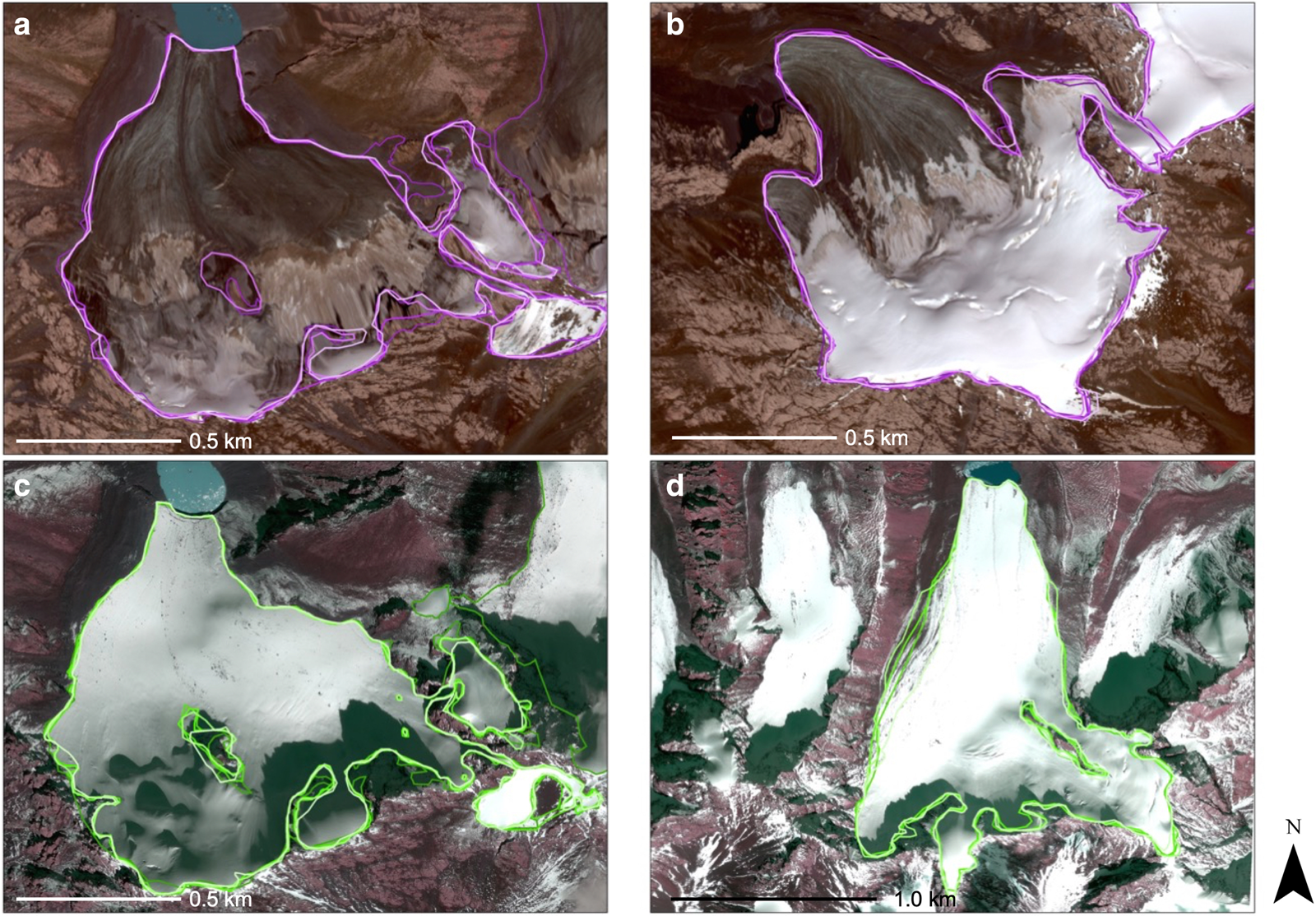
Fig. 3. Repeat delineations for the uncertainty analysis shown for (a) Glacier A in 2012 (1σ = 0.0231 km2), (b) Glacier ZN in 2012 (1σ = 0.0046 km2), (c) Glacier A in 2014 (1σ = 0.0235 km2) and (d) Glacier P in 2014 (1σ = 0.0706 km2). Sigma values represent the std dev. in surface areas calculated from the five repeat delineations for each glacier.
3.4 Glacier slope, aspect and hypsometry
All glacier elevations, slopes and aspects were derived from the highest-resolution DEM, the 1.8 m resolution SPOT-7 DEM. The values within each glacier's bounds were extracted using the 1969 glacier outlines. Following Jiskoot and others (Reference Jiskoot, Curran, Tessler and Shenton2009), the aspect values were binned into eight 45° intervals corresponding to the compass rose directions. The dominant aspect for each glacier shown in Table 2 corresponds to the bin with the greatest percentage of counts. Following a similar approach, the slopes in each glacier's boundaries were binned into 100 intervals. The most representative slope for each glacier was the bin with the greatest percentage of counts. We also report the maximum elevation and minimum elevations in the LIA, 1969, 2012 and 2014, as well as the change in minimum glacier elevation from the LIA to 2014 (Table 2).
Table 2. Surface area, direction of the dominant glacier aspect, minimum and maximum elevations (Z min and Z max), terminus elevation change (ΔZ min), Hypsometric Index (HI) and class, and area change data for the 35 glaciers measured from the LIA to 2014
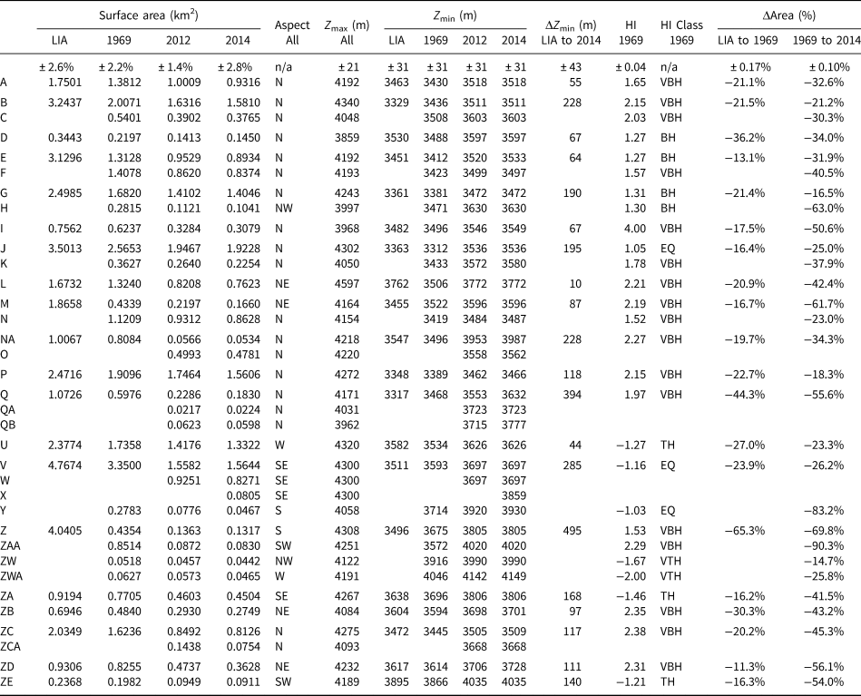
The HI classes are: very-bottom heavy (VBH), bottom-heavy (BH), equidimensional (EQ), top-heavy (TH) and very top-heavy (VTH). For glaciers that split into multiple smaller glaciers over time (e.g. Glaciers B and C), the ΔZ min from LIA to 2014 is calculated by subtracting the average of all 2014 Z min values by the Z min in the LIA. This approach for split glaciers is used for relative area change calculations as well.
We determined the hypsometric curves for each of the glacier using the distribution of elevations in each glacier's boundaries, binned into 5000 equal intervals. The cumulative sum of the surface area represented by each of the elevation intervals was used to generate the curves of elevation with respect to the normalized area. Additionally, we calculated the Hypsometric Index (HI) using the expression from Jiskoot and others (Reference Jiskoot, Curran, Tessler and Shenton2009) (Eq. 1) in order to investigate the area changes based on the hypsometric classification of the glaciers.

These HI values were used to differentiate the glaciers into five hypsometric categories: very top-heavy (HI < −1.5), top-heavy (−1.5 < HI < −1.2), equidimensional (−1.2 < HI < 1.2), bottom-heavy (HI > 1.2) and very-bottom heavy (HI > 1.5), as done in Jiskoot and others (Reference Jiskoot, Curran, Tessler and Shenton2009). Table 2 shows the HI values as well as the hypsometric categories (i.e. HI class). Uncertainties reported in Table 2 are the 95% confidence interval for the values determined from the sensitivity of the measured values to different source DEMs and the number of bins used in histogram calculations.
3.5 Total glacier area to volume and mass
Volume–area scaling relationships have been widely used in glaciology and have a strong theoretical basis (Bahr and others, Reference Bahr, Meier and Peckham1997, Reference Bahr, Pfeffer and Kaser2015). The power law scaling relationship for glaciers was derived from the models of typical glacier geometry (Bahr and others, Reference Bahr, Pfeffer and Kaser2015):

where g is ~1.36 (Frey and others, Reference Frey2014). We use the constants determined by Chen and Ohmura (Reference Chen and Ohmura1990), c = 28.5 and g = 1.357, to calculate our glacier volume. These coefficients were determined from a regression of measurements of 63 glaciers in different regions which yielded a correlation coefficient of r 2 = 0.96 (Chen and Ohmura, Reference Chen and Ohmura1990).
From glacier volume, we use a glacier ice density value, 850 ± 60 kg m−3 (Huss, Reference Huss2013), to convert volume to mass. This glacier density value accounts for the variation in density vertically throughout the glacier based on a firn compaction model, so it is lower than the density of pure ice. Wei and others (Reference Wei2015) used this value to estimate glacier mass balance from volume estimates of glaciers in Bangong Co Basin on the Tibetan Plateau. The same density value for conversion was used by Berthier and others (Reference Berthier, Cabot, Vincent and Six2016) and Brun and others (Reference Brun, Berthier, Wagnon, Kääb and Treichler2017) in studies determining glacier mass balances in the Mont-Blanc area and High Mountain Asia, respectively.
4. Results
4.1 Glacier delineations and individual glacier changes
Figure 4 shows the glacier delineations from the LIA through 2014. Additional figures showing the close-ups on outlines from a single glacier or group of glaciers are shown in the Supplementary Material (Figs S2–S6). The surface area, dominant aspect and minimum and maximum elevation for each of the 35 glaciers delineated across all dates are shown in Table 2, along with minimum elevation changes and relative area changes.

Fig. 4. LIA, 1969, 2012 and 2014 glacier outlines with Glacier ID labels. Note the variation in glacier shape and orientation as well as the retreat in their ablation zones. Glaciers without 2014 delineations lay outside the spatial extent of the 2014 Pléiades image.
4.2 Total glacier area, volume and mass changes
We report area changes from the LIA-2014 that include the total area from the 35 glaciers in Table 3. We did, however, calculate the surface area, volume and mass change for all 54 glaciers for the period 1969–2012. For the 54 glaciers, the total area change was −12.2 ± 1.0 km2, which equated to a relative area change of −30.3 ± 2.5% and a rate of change of −0.22 ± 0.02 km2 a−1 (−0.55 ± 0.02% a−1) from 1969 to 2012. This relative change is comparable to the relative change we determined for the group of 35 glaciers from 1969 to 2014 (−34.2 ± 3.5%). For the 35 glaciers, the percent glacier area, volume and mass changes were greater over the 45-year period from 1969 to 2014 than over the ~400-year period from the LIA to 1969. The percent change over just 2 years from 2012 to 2014 is one-fifth of the percent change over 45 years from 1969 to 2014. Rates of change in area, volume and mass increase over time and the average rate of change in 2012–14 (−2.1 ± 1.1% a−1 area loss) is more than 20 times faster than it was from the LIA to 1969 (−0.05 ± 0.008% a−1 area loss). Table 4 lists the total surface area, volume and mass of the glaciers delineated in the LIA, 1969, 2012 and 2014.
Table 3. Glacier surface area, volume, and mass changes for 35 glaciers from the LIA to 1969, 1969–2014 and 2012–14

ΔS is the surface area change, ΔV is the volume change and ΔM is the mass change. The percent change in mass is the same as the percent change in volume, so it is not duplicated.
Table 4. Number of glaciers delineated (N) and the total glacier surface area, volume and mass calculated for glaciers in the LIA, 1969, 2012 and 2014

5. Discussion
5.1 Glacier delineations
Processes that deviated from the GLIMS recommended methods introduced additional uncertainty to the analysis. GLIMS recommends using the same type of satellite image for each analyzed year and using the same analysis methods for each delineation set (Racoviteanu and others, Reference Racoviteanu, Paul, Raup, Khalsa and Armstrong2009). Due to changes in the suite of available high-resolution satellites over time, we relied on three different types of satellite images. Visual similarities between snow and flowing ice in the imagery complicated the identification of snowfields adjacent to the glacier, snow on the glacier and snow on top of exposed rock in the middle of glaciers. Supraglacial debris also contributed to the ambiguity of certain glacier outlines. In addition, delineation of past glacial extents was limited by the presence of moraines found in the glacial valleys. While the three characteristic LIA end moraines were identified for seven glaciers, a majority of the glaciers exhibited only one or two of the moraines in the sequence. In order to determine the LIA extents for those remaining glaciers, we relied on the location of the trim lines, which coincided with the most distal LIA end moraines. While this allowed us to draw outlines connecting end and lateral moraines as well as infer the boundary when there were no nearby moraines, this contributes to the uncertainty of our LIA outlines. The moraine sequences identified correspond to the LIA maximum date of 1586 CE ± 100 years from Li and Li (Reference Li and Li2014) and Li and others (Reference Li2016b). To account for the possibility that these features could correspond to a more recent LIA advance such as 1797–1865 CE (Liu and others, Reference Liu, Sun, Shen and Li2003), the range of the LIA dates that could be associated with these delineations is from 1486 to 1865 CE. This larger range of dates was used to project retreat rates and estimate the timing of these glaciers' disappearance. These uncertainties in delineation are reflected in our multiple digitization experiment. Interpretation of the LIA extent yielded the greatest error.
Despite these challenges, the uncertainty of all our delineated glacier areas from analyst interpretation is small compared to the glacier areas calculated. The 95% confidence interval in area calculated from multiple delineations is ±3.7% of the surface area. The std dev. of these repeat delineations ranged from 2.2 to 4.2%. This std dev. is less than the error determined by the GLIMS remote-sensing glacier digitization workshop, which yielded std dev. of 2.6–5.7% for manual delineations (Paul and others, Reference Paul2013).
5.2 Rates of glacier change
Our rates of glacier surface area loss increase over time, suggesting that glacier shrinkage is accelerating. The rate of area loss from the LIA to 1969 period was from 0.03 ± 0.005 to 0.15 ± 0.005 km2 a−1, calculated using LIA dates ranging from 1486 to 1865 CE. From 1969 to 2014, the rate of area loss was 0.22 ± 0.02 km2 a−1 and from 2012 to 2014 it was 0.60 ± 0.33 km2 a−1, at least four times and up to 20 times faster than the rate during the LIA to 1969 period (Table 3). Aizen and others (Reference Aizen, Aizen, Surazakov and Kuzmichenok2006) observed a similar trend in the acceleration of surface area loss for glaciers in the Akshiirak glacierized area in the central Tian Shan, where the rates of area loss of 0.53 ± 0.0004 km2 a−1 for the 1943–1977 period increased to a rate more than twice as fast (1.35 ± 0.001 km2 a−1) during the second period 1977–2003 (Aizen and others, Reference Aizen, Aizen, Surazakov and Kuzmichenok2006). We also provide the estimates of glacier volume and mass changes, as they respond more directly to climate forcing than surface area (Bolch and others, Reference Bolch2012; Pieczonka and Bolch, Reference Pieczonka and Bolch2015). Following the trend in the rates of surface area loss, glacier volume and mass loss are also accelerating over time. The rate of glacier volume loss from the LIA to 1969 (0.0036 ± 0.0007 km3 a−1) increased to 0.0268 ± 0.0028 km3 a−1 for the 1969–2014 period and was more than twice as fast (0.0653 ± 0.0364 km3 a−1) for the recent biennial period from 2012 to 2014. Regional climate changes, mainly increases in air temperature, may be driving these accelerations in glacier shrinkage.
From 1957 to 2014, the air temperature record from the most proximal meteorological station to our study site (Bayinbuluke) indicates a rate of warming of 0.22°C/decade and a summer temperature increase of 0.26°C/decade. The average rate of temperature change for 13 stations in Xinjiang (see Fig. 1) over that same time period is 0.23°C/decade overall and 0.14°C/decade for summer temperatures. This rate of change in Xinjiang is lower than the other reported climate trends in all of northwestern China (0.32°C/decade, Chen, Reference Chen2014), but on par with air temperature trends for China as a whole since the 1980s (0.22°C/decade, Li and others, Reference Li, Chen, Shen, Li and Xu2011b). The warming in northwestern China is approximately twice the global rate of warming of 0.26°C/decade since 1979 (IPCC, 2013). If the rise of regional air temperatures continues, glacier melt at high elevations may accelerate further and hasten desertification processes across the northwest (Aizen and others, Reference Aizen, Aizen, Surazakov and Kuzmichenok2006).
5.3 Factors influencing rapid surface area loss
The annual rate of surface area loss of all glaciers in our study area combined is 0.76 ± 0.08% a−1 from 1969 to 2014 and is higher than the range of 0.1–0.3% a−1 from the 1970s–2000s reported for glaciers with a similar size range elsewhere in the Tian Shan (Li and others, Reference Li, Li, Gao and Wang2011a). The relative glacier area loss in our study area from 1969 to 2014, 34.2 ± 3.5%, is also greater than the relative area changes determined for other glaciers in the Tian Shan (e.g. Aizen and others (2006), Li and others (2011a), Faronotti and others (2015), Osmonov and others (2013), Xu and others (2015), etc.). Reported values for relative glacier area loss elsewhere in the Tian Shan and calculated over a similar time period were lower, ranging from 10.5 to 26% (Fig. 5). Our calculated relative change in glacier area is 1.5 times greater than the values determined by Xu and others (Reference Xu2015) and is even greater than the glacier area losses calculated in the other studies, suggesting that the glaciers in our study area are losing more relative area than other glaciers in the Tian Shan (Fig. 5). Differences in average glacier size, elevation and aspect in this study area versus other study areas could also be responsible for our greater relative area losses. We examine the effect of these factors on our calculated percent area losses.

Fig. 5. Reported relative surface area changes (red points) and the time interval (grey bars) of glacier change studies in the Tian Shan. Darker red points represent greater relative area losses. Each study is labeled by author(s), study region and number of glaciers (n) in the sample. The black error bars represent the uncertainty in glacier area change for the three studies that report an uncertainty value.
5.3.1 Initial size
Average glacier size between study areas is not likely to be a primary factor influencing the inter-study differences in relative area loss. Smaller glaciers tend to lose more relative area as they recede faster (Aizen and others, Reference Aizen, Aizen and Kuzmichonok2007; Kehrl and others, Reference Kehrl, Hawley, Osterberg, Winski and Lee2014; Li and Li, Reference Li and Li2014; Li and others, Reference Li, Sun, Wang and Chen2014b; O'Neel and others, Reference O'Neel2019). In the 1960s, average glacier size in different regions of the Tian Shan ranged from 0.43 to 1.03 km2 (Li and others, Reference Li, Li, Gao and Wang2011a), while our average glacier size was 1.79 km2 in 1969 and thus larger on average than other glaciers around the Tian Shan during the 1960s. Therefore, we would expect the larger glaciers in our study site to have lost less relative area than the smaller glaciers elsewhere in the Tian Shan. However, they receded more than other Tian Shan glaciers. While average glacier size is not likely to be responsible for the inter-study differences in relative area loss, initial size does affect area loss on a glacier-by-glacier basis. For the glaciers in this study, the mean percent area loss for glaciers larger than 1 km2 (28.9%) was significantly different at the p = 0.005 level from the mean percent area loss for glaciers smaller than 1 km2 (49.8%), based on a one-way analysis of variance (ANOVA) test. The smaller glaciers experienced 20.9% more relative area loss on average than the larger glaciers (Fig. 6a). Li and others (Reference Li, Sun, Wang and Chen2014b) and Li and Li (Reference Li and Li2014) similarly found an inverse relationship between initial glacier area and relative area loss for other glaciers in the Tian Shan.

Fig. 6. (a) Initial glacier size versus percent area loss from 1969 to 2014. Dashed line indicates the separation of smaller glaciers (<1 km2 in size) versus larger glaciers (>1 km2 in size) for which the one-way ANOVA test was performed. (b) Dominant aspects versus percent area losses.
5.3.2 Aspect
Glacier aspect may be influencing our glaciers' exceptional percent area losses. At mid-latitudes in the Northern Hemisphere, north-facing glaciers receive less solar radiation than south-facing ones (Sakai and others, Reference Sakai, Nakawo and Fujita2002). As a result, south-facing glaciers in High Mountain Asia lose more relative area than north-facing glaciers (Nainwal and others, Reference Nainwal, Negi, Chaudhary, Sajwan and Gaurav2008). Li and Li (Reference Li and Li2014) found that 90.3% of 487 glaciers in the central Tian Shan are north-facing. In our study area, only 57.4% of the glaciers are north-facing and thus nearly half are exposed to greater solar radiation. However, further work must be done to connect solar radiation changes to total glacier area loss in this region. On a glacier-by-glacier basis, Li and Li (Reference Li and Li2014) found that glacier aspect was significantly correlated (at the p = 0.001 level) with area change. We similarly found a statistically significant relationship between our glaciers' dominant aspects and their area losses since 1969. The mean area loss for north-facing glaciers was significantly different at the p = 0.01 level from the mean area loss for south-facing glaciers based on a one-way ANOVA test. South-facing (S, SE and SW) glaciers underwent significantly different (p = 0.0061) losses than north-facing (N, NE and NW) glaciers (Fig. 6b). This is independent of influence from glacier size, as south-facing glaciers and north-facing glaciers did not have significantly different mean glacier sizes (p = 0.9). Mean area loss from 1969 to 2014 for south-facing glaciers was 60.8 versus 37.0% for north-facing glaciers. The difference in solar radiation experienced by glaciers with dominantly south-facing aspect is likely influencing area losses for individual glaciers as well as greater relative area loss at the basin-level.
5.3.3 Average elevation, hypsometry and surface slope
Studies in the Tian Shan, and worldwide, indicate that alpine glaciers recede more rapidly at lower elevations (Li and others, Reference Li, Li, Wang and Gao2011c; Li and Li, Reference Li and Li2014). Regional meteorological stations also indicate greater rates of summer temperature warming at lower elevations over the last half-century. From 1957 to 2014, summer air temperatures from the six stations located below 1000 m a.s.l. (Jinghe, Wusu, Yining, Kumishi, Luntai and Kuerle) increased by 0.45°C/decade on average while the Bayinbuluke station, located at 2459.4 m a.s.l., recorded a smaller 0.26°C/decade summer air temperature increase over the same period. The elevations of the glaciers in this study range from 3600 to 4200 m a.s.l., which is lower than many of the other glaciers in the Tian Shan studies shown in Figure 5. The glaciers in the Akshiirak glacierized massif and the Ala Archa glacierized basin in the Tian Shan have higher altitudinal extents of 3600–5000 and 3300–4800 m a.s.l., respectively, and lost less surface area (15.2%, Aizen and others, Reference Aizen, Aizen, Surazakov and Kuzmichenok2006) compared to our glaciers. In addition, the HI values calculated (Table 2) indicate that a majority (79%) of the glaciers in our study are bottom-heavy or very bottom-heavy, which means that more of their area is distributed at lower elevations where there are warmer temperatures and greater rates of warming, potentially contributing to their large relative area loss compared to the other studies.
While very bottom-heavy glaciers underwent greater percent area losses than very top-heavy glaciers in our study, this difference is not statistically significant. Differences in their relative area loss may be driven by other factors, such as their differences in size or surface slope, as the very top-heavy glaciers are also smaller and have steeper surface slopes (Fig. 7). Recent work has shown that surface slope is related to response time to climactic forcing, with alpine glaciers with steeper slopes responding more rapidly to climatic changes (Zekollari and others, Reference Zekollari, Huss and Farinotti2020). Analysis of relative area changes, sizes and surface slopes indicate that there is no significant correlation between dominant surface slope and size for the glaciers in this study. Meanwhile, there is a weak positive correlation between surface slope and area loss (Fig. 7d). The steeper glaciers in the study may be more sensitive to regional climatic warming and may lose their mass sooner.

Fig. 7. (a) The 35 glaciers shown by their Hypsometric Index (HI) class: very bottom-heavy (VBH), bottom-heavy (BH), equidimensional (EQ), top-heavy (TH) or very top-heavy (VTH). (b) Hypsometric curves based on normalized area for a glacier from each of the following three classes: VBH, EQ and VTH. (c) Boxplot of the average relative area changes for glaciers in each of the HI classes. (d) Surface slope versus relative area change for each glacier showing a weak positive correlation between the two variables.
5.4 Calculating a time to future disappearance
5.4.1 Linear projections
We calculated an estimate of the time for the glaciers to disappear completely using our glacier areas from the LIA through 2014. First, we calculate a disappearance year based on modern (1969–2014) glacier area change rates. We fit linear equations to the total glacier areas from 1969, 2012 and 2014 to extrapolate a conservative estimate for the end dates of our glaciers (Fig. 8). This model excludes the LIA data point, taking only the modern rate of change to determine the disappearance date. In order to capture the range of possible disappearance years due to uncertainty of the area change measurements, we performed a Monte Carlo simulation of 2000 possible linear fits based on randomly generated area values within one std dev. of the observed value (Fig. 8). The best-fit line is then determined by averaging the coefficients calculated for the 2000 simulated best-fit lines. Our linear model has limited resolving power because it is based on just 3 years of analysis.
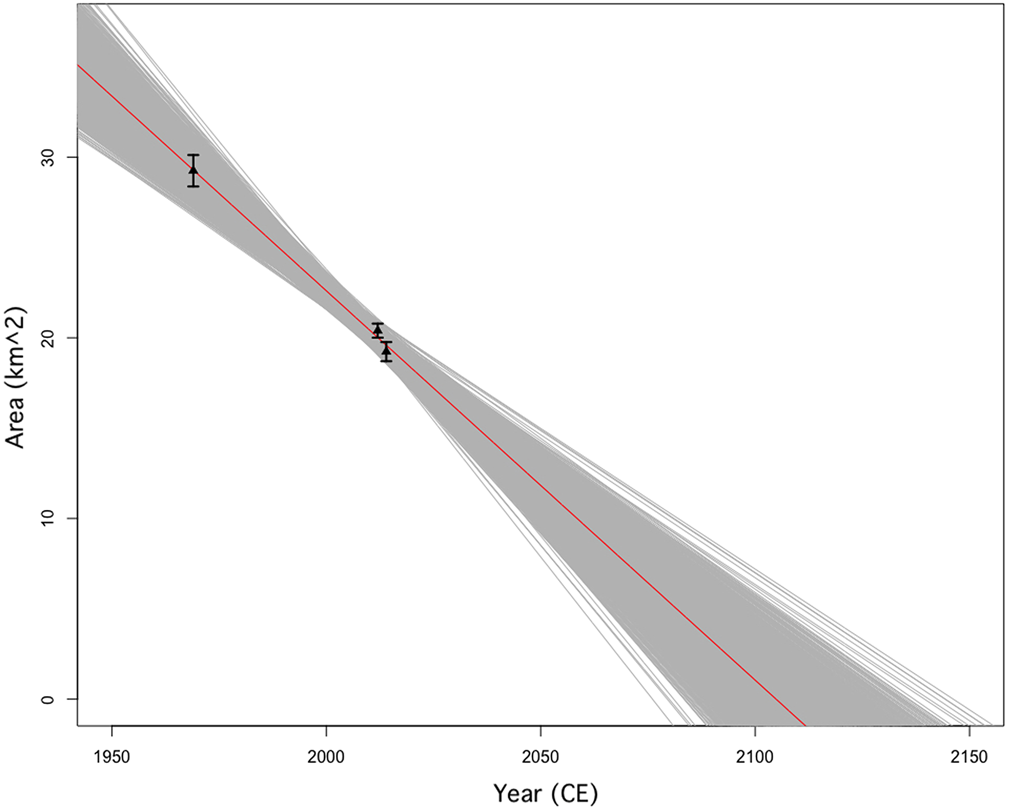
Fig. 8. Linear fits to total glacier areas for 35 glaciers from 1969, 2012 and 2014. Gray lines are linear fits generated using the 2000 variations of glacier surface area values, yielding a range of disappearance years from 2078 to 2154 CE. The best-fit line (R 2 = 0.9964) shown in red yields a disappearance year of 2106 CE.
The linear fits from the simulations yield a range of disappearance years from 2078 to 2154 CE, with a mean disappearance year of 2106 CE, based on the 1969–2014 rate of melt (−0.22 ± 0.02 km2 a−1). These estimates are in accordance with the previous estimates of the future disappearance of Himalayan and Karakoram alpine glaciers which indicate that 3000–13 000 glaciers (64–73% of the total glaciers in 1985 CE) in High Mountain Asia may disappear as early as 2035 CE if the melt rate remains at current levels (Cogley, Reference Cogley2011). To account for potential increases in melt rate due to increasing regional temperatures, we also calculate a disappearance year based on a doubled constant melt rate. With an area loss rate that is double the modern rate of area loss from 1969 to 2014, the glaciers will likely disappear in 2057 CE, nearly 50 years before the predicted disappearance year based on current melt rates (Fig. 9).

Fig. 9. The best-fit non-linear (R 2 = 0.9996) and linear models for glacier disappearance based on total glacier surface area for 35 glaciers. The linear model based on the 1969–2014 (modern) rate of area loss indicates a disappearance year of 2106 CE. The various non-linear curves generated from points within the confidence intervals for the data yield disappearance years between 2076 and 2057 CE. The latter coincides with the projection using a doubled linear melt rate, which also indicates glacier loss in ~2057 CE.
To explore the difference in potential disappearance years for the smaller glaciers (<1 km2) in our study area versus larger glaciers (>1 km2), which experience significantly greater area losses, we also calculate potential disappearance years for each of these subgroups, projecting their current rates of change into the future. For glaciers smaller than 1 km2, the rate of change in surface area from 1969 to 2014 was −1.1% a−1, yielding a disappearance year of 2048 CE. For glaciers larger than 1 km2, which lost surface area at a lower rate of −0.64% a−1 from 1969 to 2014, the disappearance is calculated to occur in 2130 CE, much later.
5.4.2 Non-linear projections
If we consider changes in ice dynamics over time, a linear model does not capture long-term changes in the rates of melt. Previous work, as well as ours, indicates that the Tian Shan glaciers have begun to retreat faster in the last four decades (Aizen and others, Reference Aizen, Aizen, Surazakov and Kuzmichenok2006). The inclusion of the LIA data point is necessary to improve the accuracy and resolving power for a non-linear fit. The best non-linear fit to the glacier areas yields the same disappearance year estimate as the doubled linear melt rate, indicating that the glaciers may disappear as early as 2057 CE, <40 years from the present (Fig. 9). The disappearance years for the glaciers in our study from all projections range from 2057 to 2154 CE, with the glaciers smaller than 1 km2 potentially disappearing even earlier in 2048 CE. Smaller glaciers respond more rapidly to climatic warming, so glaciers will melt at faster rates as they thin and their total volumes decrease (Kehrl and others, Reference Kehrl, Hawley, Osterberg, Winski and Lee2014; Li and others, Reference Li, Sun, Wang and Chen2014b). These estimates do not account for the possibility of glacier stabilization at lower volumes as the glaciers' ablation zones retreat to higher elevations (DeBeer and Sharp, Reference DeBeer and Sharp2009; Huss and others, Reference Huss, Hock, Bauder and Funk2012). While models that incorporate future climatic forcing do account for this relationship (Huss and Hock, Reference Huss and Hock2015, Reference Huss and Hock2018; IPCC, 2019; Zekollari and others, Reference Zekollari, Huss and Farinotti2019; Rounce and others, Reference Rounce, Hock and Shean2020), climate modeling is beyond the scope of our study. Our projections represent the lower bounds on the timing of glacier disappearance.
5.4.3 Hydrological response
In the case that the glaciers in our study area melt fully, a total of 2.62 ± 0.04 km3 of glacier ice (as of 2012) would be lost. The annual decrease in water volume stored in ice is equivalent to annual excess water discharge from glacier meltwater (Brun and others, Reference Brun, Berthier, Wagnon, Kääb and Treichler2017), which increases the base flow of the Kaidu River annually. Glacier meltwater is a dominant source of the Kaidu River's runoff, comprising 41–52% of the total runoff (Haiyan and others, Reference Haiyan2018). The annual discharge from meltwater will vary over time, increasing initially with glacier loss, and then will begin to decrease at a critical point (peak water) as the glaciers shrink in area and volume (Braun and others, Reference Braun, Weber and Schulz2000; Hock and others, Reference Hock, Jansson, Braun, Huber, Bugmann and Reasoner2005; IPCC, 2019). Our projections of glacier disappearance between 2057 and 2106 CE aligns with the projections of the timing of peak water. In High Mountain Asia, the timing peak water for most smaller glaciers (0–10 km2 in size) such as the glaciers in our study is projected to be between 2030 and 2040 CE for both RCP2.6 and RCP8.5 scenarios, according to a global glacier runoff model based on 14 General Circulation Models (Huss and Hock, Reference Huss and Hock2018; IPCC, 2019). This projection of timing of peak water to occur within the next two decades is a major concern for the nearby communities. The decline in runoff following peak water could ultimately result in water shortages during the dry season and considerably impact longer-term, water resource management decisions (Chen, Reference Chen2014). The decline in the Kaidu River's runoff may push communities to rely more on groundwater resources. The glacial meltwater in the upper Kaidu River basin directly affects the availability of water downstream seasonally for its potential uses, such as for human consumption, irrigation, industry, etc. Losses in glacier volume also influence the seasonal timing and variability of streamflow (Shen and others, Reference Shen, Shen, Fink, Kralisch and Brenning2018). These hydrological changes will influence future water management decisions in the region regarding intra- and inter-basin water transfers, irrigation and dam construction (Chipman and others, Reference Chipman, Shi, Magilligan, Chen and Li2016). Continued monitoring of glacier changes will be critical for determining future impacts on hydrology.
6. Conclusion
Delineations of glacier surface areas in the upper Kaidu River Basin indicate that the glaciers in this region are losing more relative area (34.2 ± 3.5%) than other glaciers in the Tian Shan (12–27%). This greater area loss may be due in part to local or regional factors including average glacier orientation and the relatively low elevations of the glaciers in the study area. Initial glacier size and dominant glacier orientation influence area losses on a glacier-by-glacier basis, with smaller glaciers and south-facing glaciers losing 20.9 and 23.8% more surface area than their counterparts, respectively. Glacial retreat is accelerating across our study area. The recent rate of glacier surface area loss (−0.60 ± 0.33 km2 a−1 from 2012 to 2014) is nearly triple the rate of surface area loss over the last half century (−0.22 ± 0.02 km2 a−1 from 1969 to 2014). Using two simple forward projections, one linear and one non-linear, we project that the glaciers may disappear as early as 2050 CE. The timeline of total glacier melt will impact water security for the communities residing in the lowlands of the Kaidu River watershed.
Supplementary material
The supplementary material for this article can be found at https://doi.org/10.1017/jog.2020.24
Acknowledgements
We thank Dr Marisa Palucis, the anonymous reviewers, Scientific Editor Neil Glasser and Associate Chief Editor Hester Jiskoot for providing comments on the manuscript that guided its revision. This research is supported by the Rockefeller Center at Dartmouth College, the Porter Family Foundation and the National Natural Science Foundation of China grants U1903208 and 41630859.
Data
Contact the corresponding author (jukes.liu@boisestate.edu) for the glacier delineations and other glacier data. For the Xinjiang weather station data, please contact Dr Yaning Chen (chenyn@ms.xjb.ac.cn) at the Xinjiang Institute of Ecology and Geography.
Author contributions
JL delineated the glaciers, performed the calculations, generated the models and figures and wrote the majority of the manuscript. DEL developed the scope and methodology of the research. He aided interpretation of geomorphic features in the images, assisted in boundary delineations, revised sections of the manuscript and provided qualitative field observations. RLH designed the method of extrapolating time to glacier disappearance and provided feedback on the research and manuscript throughout the course of the project. JC and BT obtained and processed the images and DEMs and revised the manuscript. Additionally, JC designed the Monte Carlo simulation of linear best fits for extrapolating time to glacier disappearance. This research is a component of a larger project led by XS that investigates the region's water resources and basin hydrology. YC provided oversight and climate data.


 Open access