


1 INTRODUCTION
The kinematics of the gas component of galaxies is pivotal to understanding their properties and evolutionary state at all cosmic epochs. In particular, the spatially-resolved line-of-sight gas-phase velocity dispersion (which is related to the local turbulence in the disc) obtained via integral field spectroscopy is crucial. Integral field observations of z > 1 galaxies have found high line-of-sight velocity dispersions, a factor of ~ 4–10 times larger than those of local galaxies (e.g. Genzel et al. Reference Genzel2006; Law et al. Reference Law, Steidel, Erb, Larkin, Pettini, Shapley and Wright2007; Förster Schreiber et al. Reference Schreiber2009; Wright et al. Reference Wright, Larkin, Law, Steidel, Shapley and Erb2009; Maiolino et al. Reference Maiolino2010; Epinat et al. Reference Epinat, Amram, Balkowski and Marcelin2010; Lemoine-Busserolle et al. Reference Lemoine-Busserolle, Bunker, Lamareille and Kissler-Patig2010; Gnerucci et al. Reference Gnerucci2011; Vergani et al. Reference Vergani2012; Newman et al. Reference Newman2013; Wisnioski et al. Reference Wisnioski2015). These high line-of-sight velocity dispersions suggest a turbulent inter-stellar medium. This turbulence provides support against gravitational collapse and implies that star formation should take place in large clumps which are massive enough to collapse out of this turbulent medium (Elmegreen et al. Reference Elmegreen, Elmegreen, Marcus, Shahinyan, Yau and Petersen2009). This provides an explanation for the regularly rotating but photometrically irregular (clumpy) galaxies common at z > 1 (e.g. Wisnioski et al. Reference Wisnioski, Glazebrook, Blake, Wyder, Martin, Poole and Sharp2011).
The physical mechanism(s) causing and preserving these high line-of-sight velocity dispersions remains an open question. Several possibilites have been suggested, these include gravitational instability (e.g. Bournaud et al. Reference Bournaud, Elmegreen, Teyssier, Block and Puerari2010) or generation during the initial gravitational collapse (Elmegreen & Burkert Reference Elmegreen and Burkert2010). In principle, these high velocity dispersions could be caused by feedback from star formation in the disc. However, Genzel et al. (Reference Genzel2011) found only a weak correlation between star formation and line-of-sight velocity dispersion. The high velocity dispersions are often interpreted as being consistent with, and evidence for, cold flow accretion from the inter-galactic medium at high redshift (Aumer et al. Reference Aumer, Burkert, Johansson and Genzel2010).
In contrast, observations by Green et al. (Reference Green2010, Reference Green2014) of a sample of strongly star-forming galaxies at z ~ 0.05–0.3 found that the spatially resolved line-of-sight velocity dispersion, measured from the Hα emission line, was similar to the high dispersions observed at z > 1. By combining samples spanning a range of star-formation rates and redshifts (Law et al. Reference Law, Steidel, Erb, Larkin, Pettini, Shapley and Wright2009, Reference Law, Steidel, Erb, Larkin, Pettini, Shapley and Wright2007; Yang et al. Reference Yang2008; Garrido et al. Reference Garrido, Marcelin, Amram and Boulesteix2002; Epinat et al. Reference Epinat2008b; Epinat, Amram, & Marcelin Reference Epinat, Amram and Marcelin2008a; Epinat et al. Reference Epinat2009; Lemoine-Busserolle et al. Reference Lemoine-Busserolle, Bunker, Lamareille and Kissler-Patig2010; Cresci et al. Reference Cresci2009; Contini et al., Reference Contini2012; Wisnioski et al. Reference Wisnioski, Glazebrook, Blake, Wyder, Martin, Poole and Sharp2011; Jones et al. Reference Jones, Swinbank, Ellis, Richard and Stark2010; Swinbank et al. Reference Swinbank, Smail, Sobral, Theuns, Best and Geach2012; Green et al. Reference Green2014), Green et al. (Reference Green2010, Reference Green2014) found that velocity dispersion did correlate with the star-formation rate. From this, they suggested that star formation is the energetic driver of galaxy disc turbulence at both high and low redshift. In this picture, selection effects which bias toward the most star-forming galaxies at high redshift and the rarity of such objects at low redshift result in the difference in gas phase line-of-sight velocity dispersions observed at the different epochs.
Since these measurements in general have spatial resolutions that correspond to physical scales that are significant with respect to the galaxy size, a key observational issue to be resolved is the effect of beam smearing which always acts to increase the measured dispersion on such observations. Davies et al. (Reference Davies2011) have demonstrated that biases, as a consequence of beam smearing effects, in such measurements can be severe. The sample of Green et al. (Reference Green2010) have redshifts of z ~ 0.05–0.3, which typically correspond to physical-scale resolutions of ~ 1–4 kpc (FWHM of the point spread function [PSF]). At this spatial resolution, the smearing due to convolution with the PSF can cause fundamental problems with the interpretation of spatially resolved spectroscopy (e.g. Davies et al. Reference Davies2011; Pracy, Couch, & Kuntschner Reference Pracy, Couch and Kuntschner2010). Green et al. (Reference Green2014) addressed this issue by carefully modelling the contribution of beam smearing to the observed velocity dispersion on a per spaxel basis. This technique assumes a disc model and an exponential light profile to calculate the contribution to the velocity width arising from the unresolved velocity gradient across a spatial resolution element. This correction will be valid when the disc model describes the velocity field well and the Hα flux distribution is exponential. However, the correction is not valid for non-disc galaxies or disc galaxies where the disc model does not predict the true ‘infinite resolution’ velocity field accurately. If, for example, the inner unresolved velocity gradient is steeper than the model prediction or the true Hα surface brightness is steeper than exponential then such a correction would under-predict the contribution from ‘beam smearing’. For the disc galaxies in Green et al. (Reference Green2014), they find a median correction to the flux-weighted mean of the spatially-resolved line-of-sight gas-phase velocity of just 3.6 km s−1, although in a few cases the correction is much more significant ( ~ a factor of 2).
In this paper, we present results from integral field spectroscopic observations of a small sample of six low redshift (z < 0.04) and high star-formation rate ( $\text{SFR} {\sim }10\hbox{--}40$ $\text{M}_\odot \text{ yr$^{-1}$}$
) galaxies selected from the Sloan Digital Sky Survey (SDSS; Abazajian et al. Reference Abazajian2009). While galaxies with such high star-formation rates are rare in the local Universe the wide-area, and therefore large volume at low redshift, probed by the SDSS allows the selection of a small sample of such objects. The low redshift naturally provides a good physical-scale resolution and so minimises the effects of beam smearing. In Section 2, we present details of our sample selection, observations, and data reduction. In Section 3, we outline our data analysis including emission line fitting and measuring local velocity gradients from the data. In Section 4, we present our results, including the position of our sample galaxies in the velocity dispersion-star formation plane and a simple non-parametric approach to correcting the effects of beam smearing. Throughout this paper, we convert from observed to physical units assuming a
$\text{M}_\odot \text{ yr$^{-1}$}$
) galaxies selected from the Sloan Digital Sky Survey (SDSS; Abazajian et al. Reference Abazajian2009). While galaxies with such high star-formation rates are rare in the local Universe the wide-area, and therefore large volume at low redshift, probed by the SDSS allows the selection of a small sample of such objects. The low redshift naturally provides a good physical-scale resolution and so minimises the effects of beam smearing. In Section 2, we present details of our sample selection, observations, and data reduction. In Section 3, we outline our data analysis including emission line fitting and measuring local velocity gradients from the data. In Section 4, we present our results, including the position of our sample galaxies in the velocity dispersion-star formation plane and a simple non-parametric approach to correcting the effects of beam smearing. Throughout this paper, we convert from observed to physical units assuming a $\Omega _{\text{M}}=0.3$
, ΩΛ = 0.7 and H
0 = 70 km s−1 Mpc−1 cosmology.
$\Omega _{\text{M}}=0.3$
, ΩΛ = 0.7 and H
0 = 70 km s−1 Mpc−1 cosmology.
2 SAMPLE SELECTION, OBSERVATIONS, AND DATA REDUCTION
We required a sample of high-star-formation rate and low-redshift galaxies. We selected a sample of galaxies from the SDSS with total star-formation rates above 20 M⊙ yr−1 using the MPA/JHU value added galaxy catalogue. The star-formation rates are calculated using the techniques outlined in Brinchmann et al. (Reference Brinchmann, Charlot, White, Tremonti, Kauffmann, Heckman and Brinkmann2004) and assume a Kroupa (Reference Kroupa2001) Initial Mass Function (IMF). We set a redshift limit of z = 0.04, which is a trade off between targeting galaxies as nearby as possible to gain high physical-scale resolution and having enough cosmic volume to define a reasonable number of target galaxies. At z = 0.04, 1 arcsec corresponds to just 0.8 kpc which is an improvement of ~ 2–4 over previous studies (e.g. Green et al. Reference Green2010, Reference Green2014). The spectrum for every candidate was examined by eye and spurious objects removed. The resulting catalogue contains a total of 20 galaxies fulfilling the selection criteria. Six of these objects were observable from Sidding Spring Observatory at the time of our observing run in April 2013. These six galaxies are the sample analysed in this paper. The targets have stellar masses in the range 10.5 < log (stellar mass) < 11.1 (Kauffmann et al. Reference Kauffmann2003).
A summary of our target galaxies is given in Table 1. In order to simplify comparison of the SFR from Brinchmann et al. (Reference Brinchmann, Charlot, White, Tremonti, Kauffmann, Heckman and Brinkmann2004) with literature values and our own measurements, we have converted their SFR estimates from a Kroupa (Reference Kroupa2001) to a Chabrier (Reference Chabrier2003) IMF using the relationship given in Madau & Dickinson (Reference Madau and Dickinson2014).
Table 1. Observed galaxies.

a Redshifts obtained from the Sloan Digital Sky Server (SDSS).
b Star-Formation Rate (SFR) obtained from Brinchmann et al. (Reference Brinchmann, Charlot, White, Tremonti, Kauffmann, Heckman and Brinkmann2004) and converted to a Chabrier (Reference Chabrier2003) IMF.
c Calculated from this work by summing over integral field unit (IFU) field-of-view. Assumes Chabrier (Reference Chabrier2003) IMF.
We used the Wide Field Spectrograph (WiFeS; Dopita et al. Reference Dopita, Hart, McGregor, Oates and Bloxham2007, Reference Dopita2010) on the ANU 2.3-m telescope to obtain integral field spectroscopy of our sample. They were observed over two nights on the 10th and 11th of April 2013. The total exposure time per object was between 1 and 2 h and the seeing ranged between 1.4 and 2.0 arcsec. We used the R7000 grating which delivers a spectral resolution of σ ~ 0.38Å corresponding to a velocity resolution of ~ 17 km s−1 at Hα. The wavelength range is 5 400Å < λ < 7 000Å which includes the Hα emission line at 6562.8 Å and the [NII] emission lines at 6548.1 Å and 6583.6,Å. The WiFeS has a field-of-view of 25 arcsec × 38 arcsec, which covers most of the optical extent of our target galaxies (see the left most column of Figure 1). The spaxel size is 1 arcsec.

Figure 1. Kinematic properties of the observed galaxies. From left to right: thumbnail SDSS image; along with the line-of-sight measurements of the Hα flux, velocity dispersion, velocity, and velocity gradient (left to right). The Hα flux contours with $2.5\text{log}_{10}(F_{\text{H}\alpha })$
spacing are overlaid on all the kinematic maps. The size of the seeing disc (FWHM) is illustrated by the red circle in the bottom left corner of each map.
$2.5\text{log}_{10}(F_{\text{H}\alpha })$
spacing are overlaid on all the kinematic maps. The size of the seeing disc (FWHM) is illustrated by the red circle in the bottom left corner of each map.
The data were reduced using the pywifes data reduction package (Childress et al. Reference Childress, Vogt, Nielsen and Sharp2014) which results in a fully reduced, co-added data cube. We performed a flux calibration using a matched aperture to the SDSS spectra.
3 DATA ANALYSIS
3.1. Emission line fits
For each spaxel, a triple Gaussian was fitted (using MPFIT; Markwardt Reference Markwardt2009) to the Hα emission line and the [NII] emission lines at 6548.1 Å and 6583.6 Å. The lines were fitted with a single velocity and velocity dispersion. In addition, the 6548.1 Å [NII] emission line profile was fixed at the expected ratio of 1/3rd the amplitude of the [NII] emission line at 6583.6 Å. As a result, the fit has four free parameters: the streaming velocity, velocity dispersion, and two line fluxes. The underlying continuum is taken into account by adding a linear term to the fit.
We use the best fit parameters to construct parametric maps of the Hα line flux, velocity dispersion, and streaming velocity (see columns 2, 3, and 4 of Figure 1, respectively). The instrumental resolution, σr, was subtracted in quadrature from the observed velocity dispersion for each spaxel. Low signal-to-noise spaxels were masked by requiring the estimated Hα amplitude to be greater than 2.5 × the noise (standard deviation) in the continuum. Spaxels were also masked if the provided fits to the emission lines were poor. This was done by removing spaxels where the ratio of the fitted amplitude to the actual Hα peak was less than 0.6. In addition, a limited number of individual, scattered spaxels in the outer regions were masked manually. The result of the masking can be seen in Figure 1.
3.2. Star-formation rates
To measure the integrated star formation of each galaxy, we first co-added the spectra over the entire field-of-view of the IFU and measured the line fluxes of the Hα and Hβ lines. The line fluxes were then corrected for stellar absorption following the prescription of Hopkins et al. (Reference Hopkins2003):
 $$\begin{equation}
S = {\textrm{EW} + \textrm{EW}_{c} \over \textrm{EW}} F,
\end{equation}$$
$$\begin{equation}
S = {\textrm{EW} + \textrm{EW}_{c} \over \textrm{EW}} F,
\end{equation}$$
where S is the corrected line flux of the relevant line (Hα or Hβ), EW is the equivalent width of the line, EW c is the correction for underlying stellar absorption, and F is the observed line flux. Again, following Hopkins et al. (Reference Hopkins2003), we assume EWc=1.3 Å. Next, we correct the Hα line flux for dust extinction assuming the dust extinction law of Cardelli, Clayton, & Mathis (Reference Cardelli, Clayton and Mathis1989):
 $$\begin{equation}
F(H\alpha ),\rm {corrected} = F(H\alpha ) (BD/2.86)^{2.36},
\end{equation}$$
$$\begin{equation}
F(H\alpha ),\rm {corrected} = F(H\alpha ) (BD/2.86)^{2.36},
\end{equation}$$
where BD is the Balmer Decrement: F(Hα)/F(Hβ). The Hα flux in then converted to a luminosity and the star formation rate estimated using the Kennicutt (Reference Kennicutt1998) relation and assuming a Chabrier (Reference Chabrier2003) IMF:
 $$\begin{equation}
\rm {SFR} = {L(H\alpha ) (W) \over 2.16\times 10^{34} } M\odot yr^{-1}.
\end{equation}$$
$$\begin{equation}
\rm {SFR} = {L(H\alpha ) (W) \over 2.16\times 10^{34} } M\odot yr^{-1}.
\end{equation}$$
The star-formation rates integrated over the IFU field-of-view are tabulated in Table 1.
3.3. Beam smearing and velocity gradients
Beam smearing increases the line-of-sight velocity dispersion since it mixes emission at different spatial locations, and hence different velocities, together. The magnitude of this effect depends on the local velocity gradient, in the sense that the greater the velocity gradient the greater the contribution of beam smearing to the line-of-sight velocity dispersion. We estimate the magnitude of the velocity gradient for a given spaxel vg (x, y) as the magnitude of the vector sum of the difference in the velocities in the adjacent spaxels, that is,
 $$\begin{equation}
v_{\textrm{g}}(x,y) = \sqrt{ $$\begin{array}{c}
[v(x+1,y) - v(x-1,y)]^2 \\
\qquad\quad + [v(x,y+1) - v(x,y-1)]^2. \end{array}$$ }
\end{equation}$$
$$\begin{equation}
v_{\textrm{g}}(x,y) = \sqrt{ $$\begin{array}{c}
[v(x+1,y) - v(x-1,y)]^2 \\
\qquad\quad + [v(x,y+1) - v(x,y-1)]^2. \end{array}$$ }
\end{equation}$$
Using this method, the velocity gradient is not defined for the spaxels on the edge of the field-of-view. Similarly, the velocity gradient is undefined if any of the adjacent spaxels were masked. The velocity gradient maps are shown in the right most column of Figure 1.
4 RESULTS AND DISCUSSION
4.1. Morphology in the parametric maps
In the left-most column of Figure 1, we show SDSS images of our sample. The morphologies are spiral galaxies with significant discs. In Figure 1, we compare the spatial distribution of Hα (column 2), the velocity dispersion (column 3), the streaming velocity (column 4), and the velocity gradient (column 5). For all galaxies, the line-of-sight Hα flux and velocity gradient tend to peak in the central region of each galaxy. Similarly, the observed line-of-sight velocity dispersion tends to peak in the central region of each galaxy. The exception is galaxy E which does not show a clear peaked region of the line-of-sight velocity dispersion. The observed kinematics and magnitude of the velocity gradient are related to the inclination. Galaxies E and F are less inclined than the other galaxies based on their low ellipticity and shallow rotation curves. Those galaxies have lower observed velocity dispersion and velocity gradients in their centres.
Comparison of the parametric images provide insights into how the observed velocity dispersion is effected by beam smearing and the local star-formation rate. The velocity gradient map can be used as a proxy for where broadening of the emission lines due to beam smearing should be most prominent. Since convolution with the point-spread function mixes together, a large range of velocities when the velocity gradient is large. While, the Hα line flux can be used as a direct proxy for the local star-formation rate.
It is apparent in Figure 1 that the structure in the velocity dispersion maps is better matched to the structure in the velocity gradient maps in comparison to the structure in the Hα emission line maps. For example, in Galaxy E, there is no central peak in the velocity dispersion, the velocity gradient is also relatively shallow in comparison to the other galaxies. Whereas, the Hα flux is still strongly peaked in the central region of the galaxy.
For galaxies A, B, C, D, and E, the shape of the central velocity dispersion peak corresponds more closely to the shape of the peak in velocity gradient than it does with the peak in Hα. Using galaxy B as an example, the relative Hα flux is elongated in the south-west to north-east direction. However, the galaxy has a rotation axis, and thus a line-of-sight velocity gradient peak in the south-east to north-west direction. It can be similarly seen that the velocity dispersion has a peak region that is elongated in a direction that more closely matches that of the line-of-sight velocity gradient. Another example are the non-central regions of strong Hα flux in Galaxy A which correspond to regions of constant or decreased line-of-sight velocity dispersion. Those regions also have low local velocity gradients. The morphologies of the parametric maps suggest that local enhancements in the velocity dispersion correlate more closely with the local velocity gradient than the local star-formation rate, and are suggestive of a beam smearing origin.
4.2. Statistical analysis
In Figure 2, we plot on a per spaxel basis the measured velocity dispersion versus Hα flux (left column) and the measured velocity dispersion versus the velocity gradient (Vg , right column). Each row represents a different galaxy in the sample. To more clearly illustrate the extent to which the velocity dispersion correlates with each in the F(Hα)–σ plane, we colour code each value into quartiles of the velocity gradient. While in the Vg –σ plane, we colour code each value into quartiles of the Hα flux. The quartile values are given in the legend in each panel.
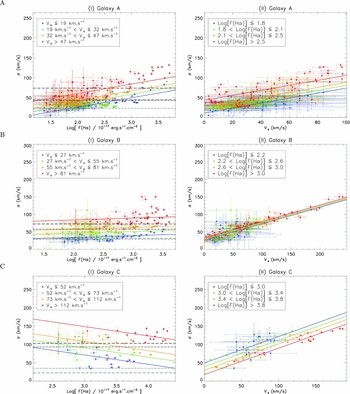
Figure 2. Each row is for a separate galaxy in the sample. Left column: The measured velocity dispersion versus Hα flux plotted for each spaxel. Right column: The measured velocity dispersion versus the velocity gradient (Vg ). To illustrate the effects of Hα flux and Vg , we colour code the spaxels into quartiles in the parameter not shown i.e. in the F(Hα)–σ plane, we colour code each value into quartiles of the velocity gradient, and in the Vg –σ plane,we colour code each value into quartiles of the Hα flux. The dashed and dot-dashed lines show the values of σ m and σ m, uni , respectively. The uncorrected measurement is shown in black (higher values) and the corrected values (i.e. Vg = 0) in grey (lower values).

For each galaxy, we fitted a 2D linear model with the velocity dispersion as the dependent variable and the Hα flux and the velocity gradient as the independent variables:
 $$\begin{eqnarray}
\sigma _i[F(\textrm{H}\alpha _i),v_{\textrm{g},i}] &=& m_{\textrm{H} \alpha } \textrm{Log}_{10}[F(\textrm{H}\alpha _i)]\nonumber\\
&&+\, m_{v_{\textrm{g}}} v_{\textrm{g},i} + C.
\end{eqnarray}$$
$$\begin{eqnarray}
\sigma _i[F(\textrm{H}\alpha _i),v_{\textrm{g},i}] &=& m_{\textrm{H} \alpha } \textrm{Log}_{10}[F(\textrm{H}\alpha _i)]\nonumber\\
&&+\, m_{v_{\textrm{g}}} v_{\textrm{g},i} + C.
\end{eqnarray}$$
The results are shown in Figure 2 and Table 2. In Figure 2, the resulting fits are shown for each quartile where the colour coded value has been held constant at its mean value in that quartile. Only four of the six galaxies show a positive correlation between velocity dispersion and Hα flux. Galaxy C and Galaxy E have a mild negative correlation, i.e. the velocity dispersion increases with decreasing Hα flux. Galaxy B and Galaxy D display mild positive correlations, while Galaxy A and Galaxy F display a highly significant positive correlation. On the other hand, in all cases, there is a significant positive correlation between the velocity dispersion and the velocity gradient (see Table 2). This implies beam smearing has a significant effect on the observed velocity dispersion even in these nearby galaxies.
Table 2. Summary of our statistical analysis of the relationship between velocity dispersion, Hα flux and local velocity gradient. Also listed are our raw and beam smearing corrected values of the velocity dispersion.

a Spearman’s rank correlation coefficient.
b Two-sided p-value from the null hypothesis ρ(A, X|Y) = 0.
c Slope for each independent variable supplied by the multiple linear regression fits.
There is a clear deviation from linear behaviour for the highest Hα fluxes in Galaxy F. At Hα fluxes above ~ 5.5 × 10⁻¹⁷ ergs s−1 cm−2, there is a sharp upturn in the velocity dispersion with increasing Hα flux which cannot be explained by increases in the velocity gradient. There is also a hint of such an upturn in Galaxy B at approximately the same flux density and at lower flux density (albeit with larger scatter) in Galaxy D. This is possible evidence for a local correlation between star-formation rate and gas velocity dispersion at the highest Hα fluxes. It is worth noting that galaxy F is the most nearby, has the smallest maximum velocity gradient and the smallest velocity dispersion (at low velocity gradient) of any galaxy. Yet, it has some of the highest Hα flux measurements. It may be that at such high SFR, star-formation feedback processes have a significant effect on the velocity dispersion, and that we can only clearly observe it in this galaxy due to the lack of beam smearing.
The linear regression analysis above is only valid if the data are well represented by a linear model. While this is generally true there are deviations from this—particularly at high Hα flux. In Table 2, we also present statistics which do not require this assumption. Specifically, we calculate the Spearman partial correlation coefficients defined as
 $$\begin{equation}
\rho _{(A,X|Y)} = \frac{\rho _{(A,X)} - \rho _{(X,Y)}\rho _{(A,Y)}}{\sqrt{(1 - \rho _{(X,Y)}^2)(1 - \rho ^2_{(A,Y)})}},
\end{equation}$$
$$\begin{equation}
\rho _{(A,X|Y)} = \frac{\rho _{(A,X)} - \rho _{(X,Y)}\rho _{(A,Y)}}{\sqrt{(1 - \rho _{(X,Y)}^2)(1 - \rho ^2_{(A,Y)})}},
\end{equation}$$
where this provides the correlation of A due to X given Y is held as a constant, along with the normalised two-sided p-value
 $$\begin{equation}
D_{(A,X|Y)} = \frac{ \sqrt{ N - 4 } }{ 2 } ln \bigg ( \frac{ 1 + \rho _{(A,X|Y)} }{ 1 - \rho _{(A,X|Y)} } \bigg ).
\end{equation}$$
$$\begin{equation}
D_{(A,X|Y)} = \frac{ \sqrt{ N - 4 } }{ 2 } ln \bigg ( \frac{ 1 + \rho _{(A,X|Y)} }{ 1 - \rho _{(A,X|Y)} } \bigg ).
\end{equation}$$
These show a similar relationship without making the assumptions required using the multiple linear regression analysis.
4.3. A simple non-parametric beam smearing correction
The linear regression models in Figure 2 suggest a means for a simple non-parametric beam smearing correction. After fitting the linear regression model, the σ value of each spaxel is taken and then corrected to v g, i = 0 based on the best fit model i.e. extrapolated to it’s value at zero velocity gradient assuming the linear model. This method avoids assumptions about the kinematics of the line-of-sight velocity and velocity dispersion fields and is much simpler than disc model fitting. Although, it does require that the data are well represented by the linear model. This correction will also be a conservative estimate since the velocity gradients are calculated from beam smeared data and the real velocity gradients will be larger.
4.4. Global velocity dispersion
The spatially resolved measurements of the velocity dispersion obtained using IFU spectroscopy can be combined into a single global velocity dispersion measurement. While reducing the parametric maps to a single value decreases the information content, it is useful in order to make comparisons between different galaxies. However, there is no unique method of constructing a single velocity dispersion value from a 2D map and as a result various measures have been used. Popular methods, and the ones that will be explored in this paper, include the flux-weighted mean σm:
 $$\begin{equation}
\sigma _{m}={\sum \nolimits _{i=1}^{n} f_{i} \sigma _{i} \over \sum _{i=1}^{n} f_{i} }
\end{equation}$$
$$\begin{equation}
\sigma _{m}={\sum \nolimits _{i=1}^{n} f_{i} \sigma _{i} \over \sum _{i=1}^{n} f_{i} }
\end{equation}$$
and a uniformly weighted mean denoted as σm, uni:
 $$\begin{equation}
\sigma _{m,uni}={\sum \nolimits _{i=1}^{n} \sigma _{i} \over n }.
\end{equation}$$
$$\begin{equation}
\sigma _{m,uni}={\sum \nolimits _{i=1}^{n} \sigma _{i} \over n }.
\end{equation}$$
Advantages of the flux weighted mean is that it up-weights high signal-to-noise spaxels; it is not sensitive to how low signal-to-noise regions in the galaxy (usually the outskirts) are masked; and since the flux of the Hα line is proportional to the star-formation rate, it is the natural way to combine the data when this is the process of interest. One disadvantage is that the star-formation rate is often greatest in the central region of the galaxy and this is also where beam smearing issues are maximal. This results in a bias towards higher global velocity dispersion (e.g. Davies et al. Reference Davies2011).
This bias can be mitigated to some extent by taking a uniformly weighted mean. However, σm, uni can be greatly affected by the imposed masking techniques. Outskirts of the galaxy will tend to have lower signal/noise affecting the accuracy in the derived kinematics. The beam smearing bias in the central region is still present and its effect increases as the signal-to-noise constraints used in masking are tightened.
In Table 2, we show our derived global velocity dispersion calculated on a flux-weighted basis using Equation (8) and a straight arithmetic mean using Equation (9). In every case, the flux-weighted mean velocity dispersion σm is larger than the arithmetic mean $\sigma _{{\rm m},\textrm{uni}}$
. The reason for this is evident from the maps in Figure 1. The Hα flux is generally centrally concentrated and this is also where the velocity field is steepest and the effect of beam smearing is maximised. Equation (8) up-weights these region producing a larger value of the velocity dispersion. We also show our values of σ
m
and σm, uni after applying our simple beam smearing correction, calculated using the best fitting solution to Equation (5) and setting
$\sigma _{{\rm m},\textrm{uni}}$
. The reason for this is evident from the maps in Figure 1. The Hα flux is generally centrally concentrated and this is also where the velocity field is steepest and the effect of beam smearing is maximised. Equation (8) up-weights these region producing a larger value of the velocity dispersion. We also show our values of σ
m
and σm, uni after applying our simple beam smearing correction, calculated using the best fitting solution to Equation (5) and setting $v_{\textrm{g},i}=0$
. The corrected values are ~ 1.5–4.5 and ~ 1.3–2.7 lower than the uncorrected values of σm and σm, uni respectively.
$v_{\textrm{g},i}=0$
. The corrected values are ~ 1.5–4.5 and ~ 1.3–2.7 lower than the uncorrected values of σm and σm, uni respectively.
In Figure 3, we plot our raw versus corrected values of σm. The points always lie above the one-to-one line since the beam smearing correction should (and does) only decrease the value of σm. For comparison, we show the sample of rotating galaxies from Green et al. (Reference Green2014). These values have been beam smearing corrected using a disc model and the assumption of an exponential light profile to calculate (on a per spaxel basis) the contribution to the velocity width arising from the unresolved velocity gradient across the spaxel. This ‘beam smearing map’ is subtracted in quadrature from the observed velocity dispersion map to produce a corrected velocity dispersion map. The velocity dispersion value is then calculated using Equation (8). The magnitude of the corrections are generally much smaller than those found using our simple linear extrapolation to zero-velocity-gradient and many of the Green et al. (Reference Green2014) galaxies lie close to the one-to-one line. The median correction being just 3.6 km s−1.

Figure 3. The uncorrected values of σ m compared to our beam smearing corrected values (black filled circles). Also shown are the sample of rotating galaxies from Green et al. (Reference Green2014), where the beam smearing correction is done using disc model fitting.
4.5. Global velocity dispersion and star-formation rate
There is an observed positive correlation between σ m and the star-formation rate which appears independent of redshift (Green et al. Reference Green2010, Reference Green2014), and this correlation has been used to argue that star formation is driving the turbulence in galaxies at all cosmic epochs. In Figure 4, we show our derived global velocity dispersion calculated on a flux-weighted basis (σm) plotted against the global star-formation rate (red crosses) calculated from summing over the entire IFU field-of-view (assumes a Chabrier (Reference Chabrier2003) IMF). We also show our values of σm after applying our simple beam smearing correction (blue crosses).

Figure 4. The star-formation rate plotted against mean velocity dispersion. Our flux weighted values (σm) are shown as red crosses. The beam smearing corrected flux weighted values (σm, v g = 0) are shown as blue crosses. A compilation of literature values are also shown with their SFRs converted to the assumption of a Chabrier (Reference Chabrier2003) IMF. Black symbols are for samples at z < 0.5 and green symbols are for objects at z > 0.5. The sample of Terlevich & Melnick (Reference Terlevich and Melnick1981) is displayed as filled black diamonds. Measurements from the GHASP survey are shown as open black circles (Epinat et al. Reference Epinat, Amram and Marcelin2008a, Reference Epinat2008b; Garrido et al. Reference Garrido, Marcelin, Amram and Boulesteix2002). The DYNAMO sample is shown as filled black hourglass symbols (Green et al. Reference Green2014). Results from the IMAGES survey (Yang et al. Reference Yang2008) are shown as filled green stars. Objects selected from the WiggleZ survey are shown as open upside-down triangles (Wisnioski et al. Reference Wisnioski, Glazebrook, Blake, Wyder, Martin, Poole and Sharp2011). The samples of Swinbank et al. (Reference Swinbank, Smail, Sobral, Theuns, Best and Geach2012) and Epinat et al. (Reference Epinat2009) are displayed as vertical filled green rectangles and horizontal filled green rectangles, respectively. Measurements from the MASSIV survey (Contini et al. Reference Contini2012) and the SINS survey (Cresci et al. Reference Cresci2009) are shown as filled green circles and open bow-tie symbols, respectively. The samples of Law et al. (Reference Law, Steidel, Erb, Larkin, Pettini, Shapley and Wright2009), Jones et al. (Reference Jones, Swinbank, Ellis, Richard and Stark2010), and Lemoine-Busserolle et al. (Reference Lemoine-Busserolle, Bunker, Lamareille and Kissler-Patig2010) are displayed as filled green diamonds, triangles, and semi-circles, respectively. Note: the σ values measured by Terlevich & Melnick (Reference Terlevich and Melnick1981) are integrated over small sub-galactic scales of ~ 10–100 pc.
Also shown in Figure 4 is a compilation of results from the literature taken from Green et al. (Reference Green2014). The star-formation rates have all been corrected for dust extinction and Green et al. (Reference Green2014) converted each to their adopted Chabrier (Reference Chabrier2003) IMF. However, the star-formation rates are derived from different indicators (e.g. Hα, SED fitting, UV luminosity) and the methods used in determining the velocity dispersions also vary.
At the lowest redshifts (z ≲ 0.01) are observations of HII regions by Terlevich & Melnick (Reference Terlevich and Melnick1981) where the velocity dispersion is a spatially integrated measurement over scales of 10–100 pc, and observations of disc galaxies in the GHASP survey (Epinat et al. Reference Epinat, Amram and Marcelin2008a, Reference Epinat2008b, Reference Epinat, Amram, Balkowski and Marcelin2010; Garrido et al. Reference Garrido, Marcelin, Amram and Boulesteix2002) which uses an unweighted mean (i.e. σm, uni). At intermediate redshift (0.4 < z < 0.75), we show the results from the IMAGES survey (Yang et al. Reference Yang2008) again using the unweighted mean. At redshifts between z = 1 and z = 2, we show the MASSIV survey (Contini et al. Reference Contini2012) and the samples of Wisnioski et al. (Reference Wisnioski, Glazebrook, Blake, Wyder, Martin, Poole and Sharp2011) and Swinbank et al. (Reference Swinbank, Smail, Sobral, Theuns, Best and Geach2012); which use a flux-weighted mean velocity dispersion. At z ~ 2–3, we show the SINS survey which uses a velocity dispersion derived from disc modelling (Cresci et al. Reference Cresci2009) which has the effect of up-weighting the outer, least beam smeared, parts of the disc. Also, at z ~ 2–3 is the sample of Epinat et al. (Reference Epinat2009) which has the average weighted by the inverse-error and the gravitationally lensed sample of Jones et al. (Reference Jones, Swinbank, Ellis, Richard and Stark2010) as well as the samples of Lemoine-Busserolle et al. (Reference Lemoine-Busserolle, Bunker, Lamareille and Kissler-Patig2010) and Law et al. (Reference Law, Steidel, Erb, Larkin, Pettini, Shapley and Wright2009); all of which used σm.
The DYNAMO survey (shown as black hourglass symbols in Figure 4) of Green et al. (Reference Green2014, uses σm) at z ~ 0.055–0.3 was designed to bridge the gap between the high- and low-redshift surveys by including galaxies with high star-formation rates similar to those at high redshift but with much better physical-scale resolution and surface brightness limits. These values have been beam smearing corrected using a disc model and the assumption of an exponential light profile as described in Section 4.4.
Our uncorrected beam smearing measurements of the mean velocity dispersion (red crosses) are in good agreement with the compilation of results from other surveys. They are consistent with the higher values of velocity dispersion at high star-formation rates and the scatter in the distribution is similar to the literature results; with values of σ m ranging from ~ 25–100 km s−1. The beam smearing corrected measurements have smaller values by a factor of ~ 2 and range from ~ 20–50 km s−1. These only overlap with the lower end of the velocity dispersion range (at similar star-formation rate) in the literature data and imply a shallower relationship between σ m and star-formation rate.
Given we expect our beam smearing correction to, in general, underestimate the true correction since it uses the observed data to calculate the velocity gradient, our data alone do not necessarily imply a positive correlation between σm and global star-formation rate. As pointed out by Green et al. (Reference Green2014) because of the large variety in the data and analysis techniques contributing to Figure 4, it is not appropriate to quantify the slope of this relation. The large difference in the slope that is implied by our corrected and uncorrected measurements and the significant scatter support the need for a more uniform set of measurements and a credible and accurate account of beam smearing across the entire parameter space.
5 SUMMARY
We have used integral field spectroscopy of a sample of six nearby, z ~ 0.01–0.04, high star-formation rate ( $\textrm{SFR} \sim 10\hbox{--}40$ $\textrm{M}_\odot \textrm{ yr$^{-1}$}$
) galaxies to investigate the relationship between velocity dispersion and star-formation rate. The low-redshift selection was made to minimise the effects of beam smearing which artificially increases the measured line-of-sight velocity dispersion by including unresolved rotation into the measured dispersion. We found:
$\textrm{M}_\odot \textrm{ yr$^{-1}$}$
) galaxies to investigate the relationship between velocity dispersion and star-formation rate. The low-redshift selection was made to minimise the effects of beam smearing which artificially increases the measured line-of-sight velocity dispersion by including unresolved rotation into the measured dispersion. We found:
-
• The contribution of beam smearing to the velocity dispersion is still significant, even at these low redshift. This is evidenced by the strong correlation between the local (spaxel by spaxel) velocity gradient (a proxy for beam smearing) and the velocity dispersion.
-
• The correlation between velocity gradient and velocity dispersion is stronger than the correlation between Hα flux (a proxy for star-formation rate) and velocity dispersion. When measured on a spaxel-by-spaxel basis, the former shows a positive correlation in all six galaxies while for the latter this is true in only four of six cases.
-
• We present a simple non-parametric beam smearing correction based on a 2D regression model of the velocity dispersion in a spaxel with respect to the velocity gradient and Hα flux and extrapolating to zero velocity gradient. This results in corrections to the velocity dispersion of a factor of ~ 1.3–4.5 and ~ 1.3–2.7 for the uncorrected flux-weighted and unweighted mean line-of-sight velocity dispersion values, respectively.
-
• The beam smearing corrected values of the mean velocity dispersion (σ m ~ 20–50 km s−1) are only marginally larger than those found in nearby low star-formation rate galaxies (σ m ~ 10–25 km s−1).
ACKNOWLEDGEMENTS
SMC acknowledges the support of an Australian Research Council Future Fellowship (FT100100457). Parts of this research were conducted by the Australian Research Council Centre of Excellence for All-sky Astrophysics (CAASTRO), through project number CE110001020. We are grateful to Adam Schaefer for helpful discussions concerning this work. We would also like to thank the anonymous referee for insightful comments which greatly improved this paper.


